BIGGREEN AT SEMEVAL-2021 TASK 1: LEXICAL COMPLEXITY PREDICTION WITH ASSEMBLY MODELS
←
→
Page content transcription
If your browser does not render page correctly, please read the page content below
BigGreen at SemEval-2021 Task 1:
                Lexical Complexity Prediction with Assembly Models

                   Aadil Islam, Weicheng Ma, Soroush Vosoughi
                          Department of Computer Science
                                Dartmouth College
    {aadil.islam.21,weicheng.ma.gr,soroush.vosoughi}@dartmouth.edu

                      Abstract                              2018) and instead measures degree of complexity
                                                            on a continuous scale. This choice is intriguing as
     This paper describes a system submitted by             it mitigates a dilemma with previous approaches
     team BigGreen to LCP 2021 for predict-                 of having to treat words extremely close to a deci-
     ing the lexical complexity of English words
                                                            sion boundary (suppose a threshold deems a word’s
     in a given context. We assemble a feature
     engineering-based model with a deep neu-               difficulty) identically to those that are far away, ie.
     ral network model founded on BERT. While               extremely easy or extremely difficult.
     BERT itself performs competitively, our fea-              Teams are asked to submit predictions on un-
     ture engineering-based model helps in extreme          labeled test sets for two subtasks: predicting on
     cases, eg. separating instances of easy and            English single word and multi word expressions
     neutral difficulty. Our handcrafted features           (MWEs). For each subtask, BigGreen presents a
     comprise a breadth of lexical, semantic, syn-
                                                            machine learning-based approach that fuses the pre-
     tactic, and novel phonological measures. Vi-
     sualizations of BERT attention maps offer in-          dictions of a feature engineering-based regressor
     sight into potential features that Transformers        with those of a feature learning-based deep neural
     models may learn when fine-tuned for lexical           network model founded on BERT (Devlin et al.,
     complexity prediction. Our ensembled predic-           2018). Our code is made available on GitHub.1
     tions score reasonably well for the single word
     subtask, and we demonstrate how they can be              2   Related Work
     harnessed to perform well on the multi word
     expression subtask too.                                Previous studies have looked at estimating the
                                                            readability of a given text at the sentence-level.
1    Introduction                                           Mc Laughlin (1969) regresses the number of poly-
                                                            syllabic words in a given lesson against the mean
Lexical simplification (LS) is the task of replacing
                                                            score for students quizzed on said lesson, yielding
difficult words in text with simpler alternatives. It
                                                            the SMOG Readability Formula. Dale and Chall
is relevant in reading comprehension, where early
                                                            (1948) offer a list of 768 (later updated to 3,000)
studies have shown infrequent words lead to more
                                                            words familiar to grade-school students in reading,
time spent by a reader fixated on it, and that ambi-
                                                            which they find correlates with passage difficulty.
guity in a word’s meaning adds to comprehension
                                                            An issue with traditional readability metrics seems
time (Rayner and Duffy, 1986). Complex word
                                                            to be the loss of generality at the word-level.
identification (CWI) is believed to be a fundamen-
tal step in the automation of lexical simplification            Shardlow (2013) tries a brute force approach
(Shardlow, 2014). Early techniques for conducting           where a simplification algorithm is applied to each
CWI suffer from a lack of robustness, from simpli-          word of a given text, deeming a word complex only
fying all words to then study its efficacy (Devlin,         if it is simplified. However, this suffers from the as-
1998), to applying thresholds on features like word         sumption that a non-complex word does not require
frequency (Zeng et al., 2005).                              further simplification. They also try assigning a fa-
   This year’s Lexical Complexity Prediction (LCP)          miliarity score to a word, and determining whether
shared task (Shardlow et al., 2021) forgoes the treat-      the word is complex or not by applying a threshold.
ment of word difficulty as a binary classification              1
                                                                  https://github.com/Aadil101/
task (Paetzold and Specia, 2016a; Yimam et al.,               BigGreen-at-LCP-2021

                                                        667
         Proceedings of the 15th International Workshop on Semantic Evaluation (SemEval-2021), pages 667–677
            Bangkok, Thailand (online), August 5–6, 2021. ©2021 Association for Computational Linguistics
Corpus Subtask Train Trial Test provided in Table 1.
Bible Single Word 2574 143 283
Multi Word 505 29 66 3.2 External Datasets
Biomed Single Word 2576 135 289 We use four additional corpora to extract term
Multi Word 514 33 53 frequency-based features from:
Europarl Single Word 2512 143 345
Multi Word 498 37 65 • English Gigaword Fifth Edition (Gigaword):
this comprises articles from seven English
Table 1: LCP train, trial, and test sets. newswires (Parker et al., 2011).
• Google Books Ngrams, version 2 (GBND):
We avoid thresholding our features in this study as this is used to count occurences of phrases
we find it unnecessary, since raw familiarity scores across a corpus of books, accessed via the
can be used as features in regression-based tasks. PhraseFinder API (Trenkmann).
Results from CWI at SemEval-2016 (Zampieri
et al., 2017) suggest vote ensembling predictions of • British National Corpus, version 3 (BNC):
the best performing models as an effective strategy, this is a collection of written and spoken En-
while several top-performing models (Paetzold and glish text (Consortium et al., 2007).
Specia, 2016b; Ronzano et al., 2016; Mukherjee
• SUBTLEXus: this consists of American En-
et al., 2016) appear to use linguistic information be-
glish subtitles, offering a multitude of word
yond just word frequency. This inspires our use of
frequency lists (Brysbaert and New, 2009).
ensemble techniques, and a foray into phonological
features as a new point of research. Results from 4 BigGreen System & Approaches
CWI at SemEval-2018 show feature engineering-
based models outperforming deep learning-based In this section, we overview features fed to our fea-
counterparts, despite the latter having generally ture engineering-based model, as well as training
better performances since SemEval-2016. techniques for the feature learning-based model.
We describe our features in detail in Appendix A.
3 Data Note that fitted models for the single word subtask
are then harnessed for the MWE subtask.
3.1 CompLex Dataset
Shardlow et al. (2020) present CompLex, a novel 4.1 Feature Engineering-based Approach
dataset in which each target expression (a single 4.1.1 Feature Extraction
word or two-token MWE) is assigned a continuous We aim to capture a breadth of information pertain-
label denoting its lexical complexity. Each label ing to the target word and its context. Most features
lies in range 0-1, and represents the (normalized) follow heavily right-skewed distributions, prompt-
average score given by employed crowd workers ing us to also consider the log-transformed version
who record an expression’s difficulty on a 5-point of each feature. For the MWE subtask, features are
Likert scale. We define a sample’s class as the extracted independently for head and tail words.
bin to which its complexity label belongs, where
bins are formed using the following mapping of 4.1.1.1 Lexical Features
complexity ranges: [0, 0.2) → 1, [0.2, 0.4) → 2,
[0.4, 0.6) → 3, [0.6, 0.8) → 4, [0.8, 1] → 5. Tar- These are features based on lexical information
get expressions in CompLex have 0.395 average about the target word:
complexity and 0.115 standard deviation, reflecting
• Word length: length of the target word.
an imbalance in favor of class 2 and 3 samples.
Each target expression is accompanied by the • Number of syllables: number of syllables in
sentence it was extracted from, drawn from one of the target word, via the Syllables library.3
three corpora (Bible, Biomed, and Europarl). A
summary of the train, trial,2 and test set samples is • Is acronym: whether the target word is a se-
2
quence of capital letters.
In our study we avoid the trial set as we find it to be less
3
representative of the training data, opting instead for training https://github.com/prosegrinder/
set cross-validation (stratified by corpus and complexity label). python-syllables
6684.1.1.2 Semantic Features 4.1.1.5 Syntactic Features
These features capture the target word’s meaning: These are features that assess the syntactic struc-
ture of the target word’s context. We construct the
• WordNet features: the number of hyponyms
constituency parse tree for each sentence using a
and hypernyms associated with the target
Stanford CoreNLP pipeline (Manning et al., 2014).
word in WordNet (Fellbaum, 2010).
• GloVe word embeddings: we extract • Part of speech (POS): tag is assigned using
300-dimension embeddings pre-trained on NLTK’s pos tag method (Bird et al., 2009).
Wikipedia-2014 and Gigaword (Pennington
• Depth of parse tree: the parse tree’s height.
et al., 2014) for each (lowercased) target word.
• ELMo word embeddings: we extract for • Depth of target word: distance (in edges) be-
each target word a 1024-dimension contex- tween target word and parse tree’s root node.
tualized embedding pre-trained on the One
• Is proper: whether the target word is a proper
Billion Word Benchmark (Peters et al., 2018).
noun/adjective, detected using capitalization.
• GloVe context embeddings: we obtain the
average 300-dimension GloVe word embed- 4.1.2 Training
ding over each token in the given sentence. Prior to training, we Z-score standardize all fea-
tures. For the single word subtask, we fit Lin-
• InferSent context embeddings: we obtain ear, Lasso (Tibshirani, 1996), Elastic Net (Zou and
4096-dimension InferSent embeddings (Con- Hastie, 2005), Support Vector Machine (Platt et al.,
neau et al., 2017) for each sentence. 1999), K-Nearest Neighbors (Wikipedia, 2021),
and XGBoost (Chen and Guestrin, 2016) regres-
4.1.1.3 Phonetic Features sion models.
These features compute the likelihood that sound- After identifying the best performing model by
able portions of the target word would arise in En- Pearson correlation, we seek to mitigate the imbal-
glish language. We estimate ground truth transition anced nature of the target variable, ie. multitude of
probabilities between any two units (phonemes or class 1,2,3 and lack of class 4,5 samples: we devise
characters) using Gigaword: a sister version of our top-performing model, fit
upon a reduced training set. For the reduced set,
• Phoneme transition probability: we con- we tune percentages removed from classes 1-3 by
sider the min/max/mean/standard deviation performing cross-validation on the full training set.
over the set of transition probabilities for the
target word’s phoneme bigrams. 4.2 Approach based on Feature Learning
• Character transition probability: analogous Our handcrafted feature set relies heavily on target
to that above, over character bigrams. word-specific features. Beyond N-gram and syntac-
tic features, it is a cursory analysis of the context
4.1.1.4 Word Frequency & N-gram Features surrounding the target word. We seek an alterna-
tive, automated approach using feature learning.
These features are expressly included due to their
expected importance as features (Zampieri et al., 4.2.1 Architecture
2017). Gigaword is the main corpus from which LSTM-based approaches have been used to model
we extract word frequency measures (for both lem- the contexts of target words in past works (Hart-
matized and unlemmatized versions of the target mann and Dos Santos, 2018; De Hertog and Tack,
word), summed frequency of the target word’s byte 2018). An issue with a single LSTM is its ability to
pair encodings (BPEs), as well as summed frequen- read tokens of an input sentence sequentially only
cies of bigrams and trigrams. We complement these in a single direction (eg. left-to-right). It inspires
features with their IDF-based analogues. Lastly, we us to try a Transformer-based approach (Vaswani
use the GBND, BNC, and SUBTLEXus corpora et al., 2017), architectures that process sentences as
to extract secondary word frequency, bigram, and a whole (instead of word-by-word) by applying at-
trigram measures. tention mechanisms upon them. Attention weights
669are useful as they can be interpreted as learned re- Model Pearson Rank
lationships between words. BERT (Devlin et al., XGBoostfull 0.7589 -
2018) is one such model used for a variety of natu- XGBoostreduced 0.7456 -
ral language understanding (NLU) tasks. XGBoostfull+reduced 0.7576 -
Multi-Task Deep Neural Network (MT-DNN) MT-DNN 0.7484 -
proposed by Liu et al. (2019) offers state-of-the- Ensemble (submission) 0.7749 8/54
art results for multiple NLU tasks by incorporat- Best competition results 0.7886
ing benefits of both multi-task learning and lan-
guage model pre-training. We are able to initialize Table 2: Test set results for single word subtask.
MT-DNN’s shared text encoding layers with a pre-
Model Pearson Rank
trained BERT base model (cased), and fine-tune
XGBoostfull+red. (head) 0.7164 -
its later layers for 5 epochs, using a mean squared
XGBoostfull+red. (tail) 0.7188 -
error loss function and default hyperparameters.
MT-DNN 0.7890 -
Such hyperparameter settings are provided in Ap-
Ensemble (submission) 0.7898 25/37
pendix B. Note that the model is fine-tuned on only
Ensemble (improved) 0.8290 *14/37
the CompLex corpus.
Best competition results 0.8612
4.2.2 Input Layer
Table 3: MWE subtask test set results. (*projection)
Data is fed to the model’s input layer in Premise-
AndOneHypothesis format, premise and hypothesis
being sentence and target word/MWE, respectively. 6 Analysis
The data is preprocessed by a BERT tokenizer,
backed by Hugging Face (Wolf et al., 2020). 6.1 Performance
For feature selection, we find success in selecting
4.2.3 Output Layer
the top-300 features by mutual information and
Our model’s output layer produces the predicted removing quasi-constant features. The pruned fea-
lexical complexity for a given target word/MWE. ture set is passed to wrapper/embedded methods
Additionally, we extract attention maps across each and a variety of regressors for model comparison.
of the model’s attention heads, for each test set We find an XGBoost regressor (with hyperparame-
sample. These will be assessed in Section 6.3. ters tuned via grid search) to excel consistently for
4.3 Ensembling the single word subtask. As shown in Table 2, we
rank in the top 15% by Pearson correlation.
Our best performing feature engineering-based re- For the MWE subtask, performances are re-
gression model yields two sets of predictions (from ported in Table 3. Note that our submitted pre-
fitting on full and reduced training sets, respec- dictions differ from post-competition predictions.
tively). We default to using the full predictions, We previously used a training procedure resem-
then tune a threshold, where predictions higher than bling that for the single word subtask: (1) filter
the threshold (likely of class 4,5 samples) are over- methods for feature selection, (2) XGBoost for re-
written with the reduced predictions. We compute gression, (3) ensembling with MT-DNN. We had
a weighted average ensemble of these predictions passed the entire MWE as input to our XGBoost
with those of our MT-DNN model to obtain a final and MT-DNN models. We hypothesize that the
set of predictions for the single word subtask. fewer number of training samples available for this
For the MWE subtask, the fitted models from the subtask contributed to the prior procedure’s lack-
previous subtask are harnessed to predict lexical luster performance. This inspired us to incorporate
complexities for the head and tail words. We then the predictive capabilities of our fitted single word
compute a weighted average ensemble of these subtask models by applying them independently on
predicted complexities and the predictions of an the MWE’s constituent head and tail words. This
MT-DNN model trained on MWEs. gives us predicted complexities for the head and tail
words each, which when ensembled with the pre-
5 Results
dictions of our MT-DNN model (that, mind you, is
We present the performances of BigGreen’s sys- trained on the entire MWE) yields superior results
tem on each subtask in Tables 2 and 3. to those submitted to competition.
670Figure 1: Feature importances for XGBoostfull .
Definitions of the features are shown in Appendix A.
Figure 3: Head 3-9 attention map for a random sample.
6.3 BERT Attention
Attention maps have in previous works been
assessed to demonstrate linguistic phenomena
learned by a Transformer’s specialized attention
heads (Voita et al., 2019; Clark et al., 2019). We
extract attention maps from MT-DNN’s underlying
fine-tuned BERT architecture. For each sample in
the single word test set, we obtain an attention map
from each of the BERT base model’s 144 attention
heads (ie. 12 heads per 12 layers).
Based on the precedence given to term frequency
features by the XGBoostfull model, we hypothe-
size that for certain attention heads, the degree to
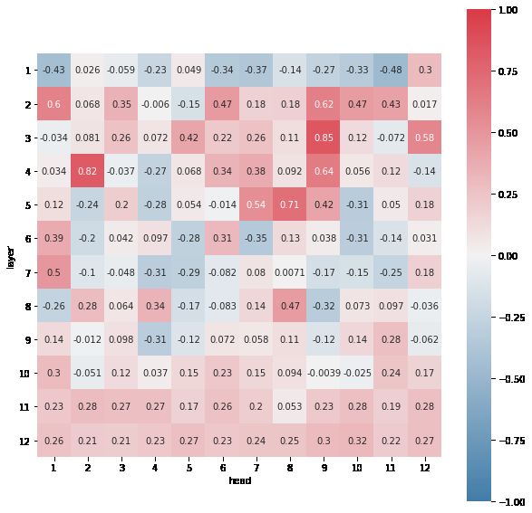
Figure 2: Attention head correlation between word which BPEs attend to one another varies relative to
frequency and total attention received by word, their word’s rarity in lexicon. This follows the find-
averaged across 100 random test set samples. ings of Voita et al. (2019), who identify heads in
which lesser frequent tokens are attended to semi-
uniformly by a majority of sentence tokens.
6.2 Feature Contribution To test our hypothesis, we estimate for each at-
tention head the Pearson correlation between word
In total we consider 110 features, in addition to frequency and average attention given to each word
our multidimensional embedding-based features in the context.4 As illustrated in Figure 2, we find
and log-transformed features. We inspect the esti- multiple attention heads appearing to specialize at
mated feature importance scores produced by the directing attention towards the most or least fre-
XGBoostfull model to find that term frequency- quent words (depending on sign of the correlation).
based features (eg. unigrams, bigrams, trigrams) Vertical stripe patterns like that in Figure 3 emerge
are of overwhelming importance (see Figure 1). as a result of attention originating from a spectrum
This raises concern for whether the MT-DNN of tokens. The findings seem to affirm the fun-
model too relies on term frequencies to make its damental relevancy of word frequency to lexical
predictions, and if not, the linguistic features it may complexity prediction, corroborating our intuition.
have learned upon fine-tuning. Of the remaining
4
features having non-zero feature importances, most We compute attention given to a word as the sum of
attention given to its constituent BPEs. We use the GBND
appear to be dimensions of target word-based se- corpus to extract word frequencies, though any large corpora
mantic features (ie. GloVe or ELMo embeddings). would suffice.
6717 Conclusion natural language inference data. arXiv preprint
arXiv:1705.02364.
In this paper, we report inspirations for a system
submitted by BigGreen to LCP SharedTask 2021, BNC Consortium et al. 2007. British national corpus.
performing reasonably well for the single word sub- Oxford Text Archive Core Collection.
task by adapting ensemble methods upon feature Edgar Dale and Jeanne S Chall. 1948. A formula for
engineering and feature learning-based models. We predicting readability: Instructions. Educational re-
see potential in future deep learning approaches, search bulletin, pages 37–54.
acknowledging the need for complementary word
Dirk De Hertog and Anaı̈s Tack. 2018. Deep Learn-
frequency-based handcrafted features for the time ing Architecture for ComplexWord Identification. In
being. We surpass our submitted results for the Thirteenth Workshop of Innovative Use of NLP for
MWE subtask, by utilizing the predictive capabili- Building Educational Applications, pages 328–334.
ties of our single word subtask models. Association for Computational Linguistics (ACL);
New Orleans, Louisiana.
Avenues for improvement include better data ag-
gregation, as a relative lack of class 4,5 samples Jacob Devlin, Ming-Wei Chang, Kenton Lee, and
seems to hurt Pearson correlation across extremely Kristina Toutanova. 2018. BERT: Pre-training of
complex samples. An approach may involve syn- deep bidirectional transformers for language under-
standing. arXiv preprint arXiv:1810.04805.
thetic data generation using SMOGN (Branco et al.,
2017). Shardlow et al. (2020) acknowledge a Siobhan Devlin. 1998. The use of a psycholinguistic
reader’s familiarity with a genre may affect per- database in the simplification of text for aphasic read-
ceived word complexity. However, the CompLex ers. Linguistic databases.
dataset lacks information on each annotator’s ex- Christiane Fellbaum. 2010. WordNet. In Theory and ap-
pertise or background, which may offer valuable plications of ontology: computer applications, pages
new insights. 231–243. Springer.
Nathan Hartmann and Leandro Borges Dos Santos.
2018. NILC at CWI 2018: Exploring feature en-
References gineering and feature learning. In Proceedings of the
Steven Bird, Ewan Klein, and Edward Loper. 2009. Nat- Thirteenth Workshop on Innovative Use of NLP for
ural language processing with Python: analyzing text Building Educational Applications, pages 335–340.
with the natural language toolkit. O’Reilly Media,
Inc. Michael Lesk. 1986. Automatic sense disambiguation
using machine readable dictionaries: how to tell a
Paula Branco, Luı́s Torgo, and Rita P Ribeiro. 2017. pine cone from an ice cream cone. In Proceedings of
SMOGN: A pre-processing approach for imbalanced the 5th annual international conference on Systems
regression. In First international workshop on learn- documentation, pages 24–26.
ing with imbalanced domains: Theory and applica-
tions, pages 36–50. PMLR. Xiaodong Liu, Pengcheng He, Weizhu Chen, and Jian-
feng Gao. 2019. Multi-task deep neural networks
Marc Brysbaert and Boris New. 2009. Moving beyond for natural language understanding. arXiv preprint
Kučera and Francis: A critical evaluation of current arXiv:1901.11504.
word frequency norms and the introduction of a new
and improved word frequency measure for American Christopher D Manning, Mihai Surdeanu, John Bauer,
English. Behavior research methods, 41(4):977–990. Jenny Rose Finkel, Steven Bethard, and David Mc-
Closky. 2014. The Stanford CoreNLP natural lan-
Tianqi Chen and Carlos Guestrin. 2016. XGBoost: A guage processing toolkit. In Proceedings of 52nd
scalable tree boosting system. In Proceedings of annual meeting of the association for computational
the 22nd acm sigkdd international conference on linguistics: system demonstrations, pages 55–60.
knowledge discovery and data mining, pages 785–
794. G Harry Mc Laughlin. 1969. SMOG grading-a new
readability formula. Journal of reading, 12(8):639–
Kevin Clark, Urvashi Khandelwal, Omer Levy, and 646.
Christopher D Manning. 2019. What Does BERT
Look At? An Analysis of BERT’s Attention. arXiv Niloy Mukherjee, Braja Gopal Patra, Dipankar Das, and
preprint arXiv:1906.04341. Sivaji Bandyopadhyay. 2016. JUNLP at SemEval-
2016 Task 11: Identifying complex words in a sen-
Alexis Conneau, Douwe Kiela, Holger Schwenk, Loic tence. In Proceedings of the 10th International Work-
Barrault, and Antoine Bordes. 2017. Supervised shop on Semantic Evaluation (SemEval-2016), pages
learning of universal sentence representations from 986–990.
672Gustavo Paetzold and Lucia Specia. 2016a. SemEval Matthew Shardlow, Richard Evans, Gustavo Paetzold,
2016 Task 11: Complex word identification. In Pro- and Marcos Zampieri. 2021. SemEval-2021 Task 1:
ceedings of the 10th International Workshop on Se- Lexical Complexity Prediction. In Proceedings of the
mantic Evaluation (SemEval-2016), pages 560–569. 14th International Workshop on Semantic Evaluation
(SemEval-2021).
Gustavo Paetzold and Lucia Specia. 2016b. SV000GG
at SemEval-2016 Task 11: Heavy gauge complex Robert Tibshirani. 1996. Regression shrinkage and se-
word identification with system voting. In Proceed- lection via the lasso. Journal of the Royal Statistical
ings of the 10th International Workshop on Semantic Society: Series B (Methodological), 58(1):267–288.
Evaluation (SemEval-2016), pages 969–974.
Martin Trenkmann. PhraseFinder – search millions of
R Parker, D Graff, J Kong, K Chen, and K Maeda. 2011. books for language use. https://phrasefinder.
English Gigaword Fifth Edition LDC2011T07 (tech. io. Accessed: 2021-02-08.
rep.). Technical report, Technical Report. Linguistic
Data Consortium, Philadelphia. Ashish Vaswani, Noam Shazeer, Niki Parmar, Jakob
Uszkoreit, Llion Jones, Aidan N Gomez, Lukasz
Fabian Pedregosa, Gaël Varoquaux, Alexandre Gram- Kaiser, and Illia Polosukhin. 2017. Attention is all
fort, Vincent Michel, Bertrand Thirion, Olivier Grisel, you need. arXiv preprint arXiv:1706.03762.
Mathieu Blondel, Peter Prettenhofer, Ron Weiss, Vin-
cent Dubourg, et al. 2011. Scikit-learn: Machine Elena Voita, David Talbot, Fedor Moiseev, Rico Sen-
learning in Python. The Journal of Machine Learn- nrich, and Ivan Titov. 2019. Analyzing multi-
ing Research, 12:2825–2830. head self-attention: Specialized heads do the heavy
lifting, the rest can be pruned. arXiv preprint
Jeffrey Pennington, Richard Socher, and Christopher D arXiv:1905.09418.
Manning. 2014. GloVe: Global vectors for word rep-
resentation. In Proceedings of the 2014 conference Wikipedia. 2021. K-nearest neighbors algo-
on empirical methods in natural language processing rithm — Wikipedia, the free encyclope-
(EMNLP), pages 1532–1543. dia. http://en.wikipedia.org/w/index.
php?title=K-nearest%20neighbors%
Matthew E Peters, Mark Neumann, Mohit Iyyer, Matt
20algorithm&oldid=1008084290. [Online;
Gardner, Christopher Clark, Kenton Lee, and Luke
accessed 02-April-2021].
Zettlemoyer. 2018. Deep contextualized word repre-
sentations. arXiv preprint arXiv:1802.05365. Thomas Wolf, Julien Chaumond, Lysandre Debut, Vic-
John Platt et al. 1999. Probabilistic outputs for support tor Sanh, Clement Delangue, Anthony Moi, Pier-
vector machines and comparisons to regularized like- ric Cistac, Morgan Funtowicz, Joe Davison, Sam
lihood methods. Advances in large margin classifiers, Shleifer, et al. 2020. Transformers: State-of-the-
10(3):61–74. art natural language processing. In Proceedings of
the 2020 Conference on Empirical Methods in Nat-
Keith Rayner and Susan A Duffy. 1986. Lexical com- ural Language Processing: System Demonstrations,
plexity and fixation times in reading: Effects of word pages 38–45.
frequency, verb complexity, and lexical ambiguity.
Memory & cognition, 14(3):191–201. Seid Muhie Yimam, Chris Biemann, Shervin Malmasi,
Gustavo H Paetzold, Lucia Specia, Sanja Štajner,
Francesco Ronzano, Luis Espinosa Anke, Horacio Sag- Anaı̈s Tack, and Marcos Zampieri. 2018. A report
gion, et al. 2016. TALN at SemEval-2016 Task 11: on the complex word identification shared task 2018.
Modelling complex words by contextual, lexical and arXiv preprint arXiv:1804.09132.
semantic features. In Proceedings of the 10th Interna-
tional Workshop on Semantic Evaluation (SemEval- Marcos Zampieri, Shervin Malmasi, Gustavo Paetzold,
2016), pages 1011–1016. and Lucia Specia. 2017. Complex word identifica-
tion: Challenges in data annotation and system per-
Matthew Shardlow. 2013. A Comparison of Tech- formance. arXiv preprint arXiv:1710.04989.
niques to Automatically Identify Complex Words.
In 51st Annual Meeting of the Association for Com- Qing Zeng, Eunjung Kim, Jon Crowell, and Tony Tse.
putational Linguistics Proceedings of the Student 2005. A text corpora-based estimation of the famil-
Research Workshop, pages 103–109. iarity of health terminology. In International Sympo-
sium on Biological and Medical Data Analysis, pages
Matthew Shardlow. 2014. Out in the Open: Finding 184–192. Springer.
and Categorising Errors in the Lexical Simplification
Pipeline. In LREC, pages 1583–1590. Hui Zou and Trevor Hastie. 2005. Regularization and
variable selection via the elastic net. Journal of the
Matthew Shardlow, Michael Cooper, and Marcos royal statistical society: series B (statistical method-
Zampieri. 2020. CompLex: A New Corpus for Lex- ology), 67(2):301–320.
ical Complexity Predicition from Likert Scale Data.
In Proceedings of the 1st Workshop on Tools and
Resources to Empower People with REAding DIffi-
culties (READI).
673A Feature Descriptions A.3 Phonetic Features
Here, we describe in greater detail the various fea- char transition min
tures that were experimented with for our feature
• Minimum of the set of character transition
engineering-based model. Note that while this dis-
probabilities for each character bigram in the
cussion regards the single word subtask, for the
target word. Ground truth character transition
MWE subtask we compute the same features but
probabilities between any two English charac-
for each of the head and tail words, respectively.
ters are estimated over Gigaword.
A.1 Lexical Features
char transition max
word len
• Maximum of the set described above.
• Character length of the target word.
num syllables char transition mean
• Number of syllables in the target word, via • Mean of the set described above.
the Syllables library.
char transition std
is acronym
• Standard deviation of the set described above.
• Boolean for whether the target word is all
capital letters. phoneme transition min
A.2 Semantic Features
• Minimum of the set of phoneme transition
num hyperyms probabilities for each character bigram in the
• Number of hyperyms associated with the tar- target word. Ground truth phoneme transi-
get word. The target word is initially dis- tion probabilities between any two phonemes
ambiguated using NLTK’s implementation of are estimated over the Gigaword corpus. The
the Lesk algorithm for Word Sense Disam- phoneme set considered is that of the CMU
biguation (WSD) (Lesk, 1986), which finds Pronouncing Dictionary.5
the WordNet Synset with the highest number
phoneme transition max
of overlapping words between the context and
different definitions of each Synset. • Maximum of the set described above.
num hyponyms phoneme transition mean
• Number of hyponyms associated with the tar-
• Mean of the set described above.
get word. Procedure for finding this is analo-
gous to that for num hyperyms. phoneme transition std
glove word
• Standard deviation of the set described above.
• 300-dimension embedding for each target
word, pre-trained on Wikipedia-2014 and Gi- A.4 Word Frequency & N-gram Features
gaword. Target word is lowercased for ease. A.4.1 Gigaword-based
elmo word tf
• 1024-dimension embedding for each target • Target word term frequency. Note that all term
word, pre-trained on the One Billion Word frequency-based features are computed using
Benchmark corpus. Scikit-learn library’s CountVectorizer
glove context (Pedregosa et al., 2011).
• 300-dimension average of GloVe word em- tf lemma
beddings (see glove word above) for each
word in the given context. Each word is low- • Term frequency of the lemmatized target word.
ercased for simplicity. Lemmatization is performed using NLTK’s
WordNet Lemmatizer.
infersent embeddings 5
http://speech.cs.cmu.edu/cgi-bin/
• 4096-dimension embedding for the context. cmudict
674tf summed bpe • Standard deviation of the set described above.
• Sum of term frequencies of each BPE in the google ngram 3 head
target word. BPE tokenization is performed
• Term frequency of leading trigram in the con-
using Hugging Face’s BERT Tokenizer.
text containing the target word.
tf ngram 2
google ngram 3 mid
• Sum of the term frequencies of each bigram
• Term frequency of middle trigram in the con-
in the context containing the target word.
text containing the target word.
tf ngram 3
google ngram 3 tail
• Sum of the term frequencies of each trigram
• Term frequency of trailing trigram in the con-
in the context containing the target word.
text containing the target word.
tfidf
google ngram 3 min
• Term frequency-inverse document frequency.
• Minimum of set of term frequencies of tri-
tfidf ngram 2 grams in the context containing target word.
• Sum of the term frequency-inverse document google ngram 3 max
frequencies of each bigram in the context con-
• Maximum of the set described above.
taining the target word.
google ngram 3 mean
tfidf ngram 3
• Average of the set described above.
• Sum of the term frequency-inverse document
frequencies of each trigram in the context con- google ngrams 3 std
taining the target word.
• Standard deviation of the set described above.
A.4.2 Google N-gram-based
A.4.3 SUBTLEXus-based
google ngram 1
FREQcount
• Term frequency of the target word.
• Number of times target word appears in cor-
google ngram 2 head pus.
• Term frequency of leading bigram in the con- CDcount
text containing the target word.
• Number of films in which target word appears.
google ngram 2 tail
FREQlow
• Term frequency of trailing bigram in the con-
text containing the target word. • Number of times the lowercased target word
appears in corpus.
google ngram 2 min
CDlow
• Minimum of the set of term frequencies of
bigrams in context containing the target word. • Number of films in which the lowercased tar-
get word appears.
google ngram 2 max
SUBTLWF
• Maximum of the set described above.
• Number of times the target word appears per
google ngram 2 mean million words.
• Average of the set described above. SUBTLCD
google ngram 2 std • Percent of films in which target word appears.
675A.4.4 BNC-based A.7 Other Features
bnc frequency: Target word term frequency. ppl
A.5 Syntactic Features
• Perplexity metric, as defined by the Hugging
parse tree depth
Face library.7 For each token in the context,
• Height of context’s constituency parse tree. we use a pre-trained GPT-2 model to estimate
Parse trees are obtained using a Stanford the log-likelihood of the token occurring given
CoreNLP pipeline. its preceding tokens. A sliding-window ap-
token depth proach is used to handle the large number of
tokens in a context. The log-likelihoods are
• Depth of the target word with respect to root
averaged, and then exponentiated.
node of the context’s constituency parse tree.
num words at depth ppl aspect only
• Number of words at the depth of the target
word (see token depth above) in the con- • Similar approach to that described above,
text’s constituency parse tree. where only log-likelihoods of tokens compris-
ing the target word are averaged.
is proper
• Boolean for whether target word is a proper num OOV
noun/adjective, based on capitalization.
POS {CC, CD, DT, EX, FW, IN, JJ, • Number of words in the context that do not
JJR, JJS, LS, MD, NN, NNP, NNPS, exist in the vocabulary of Gigaword.
NNS, PDT, POS, PRP, PRP$, RB,
RBR, RBS, RP, SYM, TO, UH, VB, corpus bible, corpus biomed,
VBD, VBG, VBN, VBP, VBZ, WDT, WP, corpus europarl
WP$, WRB}
• Booleans indicating the sample’s domain.
• Booleans indicating the target word’s part-of-
speech tag. Tags considered are those used
in the Penn Treebank Project.6 Tags are esti-
B Model Hyperparameters
mated using NLTK’s pos tag method. Here we provide optimized hyperparameter set-
A.6 Readability Features tings that may help future developers with repro-
automated readability index, ducing results, namely with training our models.
avg character per word,
avg letter per word, B.1 XGBoost
avg syllables per word, Below are tuned parameters used for all of our
char count, coleman liau index, XGBoost models. Parameters not listed are given
crawford, fernandez huerta, default values as specified in documentation:8
flesch kincaid grade, colsample bytree: 0.7
flesch reading ease, learning rate: 0.03
gutierrez polini, max depth: 5
letter count, lexicon count, min child weight: 4
linsear write formula, lix, n estimators: 225
polysyllabcount, reading time, nthread: 4
rix, syllable count, objective: ‘reg:linear’
szigriszt pazos, SMOGIndex, silent: 1
DaleChallIndex subsample: 0.7
• Algorithms applied using Textstat library im- 7
https://huggingface.co/transformers/
plementations, most being readability metrics. perplexity.html
6 8
https://www.ling.upenn.edu/courses/ https://xgboost.readthedocs.io/en/
Fall_2003/ling001/penn_treebank_pos.html latest/
676B.2 MT-DNN
MT-DNN uses yaml as its config file format. Be-
low are the contents of our task config file:
data format: PremiseAndOneHypothesis
enable san: false
metric meta:
- Pearson
- Spearman
n class: 1
loss: MseCriterion
kd loss: MseCriterion
adv loss: MseCriterion
task type: Regression
B.3 Ensemble
Threshold above which a sample is assigned its
reduced prediction (ie. XGBoostreduced prediction)
instead of its full prediction (ie. XGBoostfull
prediction): 0.59. Note that this threshold is used
to compute our XGBoostfull+reduced prediction.
Weighted average ensemble (single word subtask):
- Weight for XGBoostfull+reduced prediction: 0.5
- Weight for MT-DNN prediction: 0.5
Weighted average ensemble (MWE subtask):
- Weight for XGBoostfull+reduced (head): 0.28
- Weight for XGBoostfull+reduced (tail): 0.17
- Weight for MT-DNN prediction: 0.55
677You can also read