Deep Sound Field Reconstruction in Real Rooms: Introducing the ISOBEL Sound Field Dataset - arXiv
←
→
Page content transcription
If your browser does not render page correctly, please read the page content below
Deep Sound Field Reconstruction in Real Rooms:
                                         Introducing the ISOBEL Sound Field Dataset
                                                  Miklas Strøm Kristoffersen,1, 2 Martin Bo Møller,1 Pablo Martı́nez-Nuevo,1 and Jan Østergaard2
                                                  1
                                                      Research Department, Bang & Olufsen a/s, Struer, Denmark
                                                  2
                                                      AI and Sound Section, Department of Electronic Systems, Aalborg University, Aalborg, Denmark
                                                  Knowledge of loudspeaker responses are useful in a number of applications, where a sound
                                                  system is located inside a room that alters the listening experience depending on position
                                                  within the room. Acquisition of sound fields for sound sources located in reverberant rooms
                                                  can be achieved through labor intensive measurements of impulse response functions covering
                                                  the room, or alternatively by means of reconstruction methods which can potentially require
                                                  significantly fewer measurements. This paper extends evaluations of sound field reconstruc-
                                                  tion at low frequencies by introducing a dataset with measurements from four real rooms.
arXiv:2102.06455v1 [cs.SD] 12 Feb 2021

                                                  The ISOBEL Sound Field dataset is publicly available, and aims to bridge the gap between
                                                  synthetic and real-world sound fields in rectangular rooms. Moreover, the paper advances on
                                                  a recent deep learning-based method for sound field reconstruction using a very low number
                                                  of microphones, and proposes an approach for modeling both magnitude and phase response
                                                  in a U-Net-like neural network architecture. The complex-valued sound field reconstruction
                                                  demonstrates that the estimated room transfer functions are of high enough accuracy to
                                                  allow for personalized sound zones with contrast ratios comparable to ideal room transfer
                                                  functions using 15 microphones below 150 Hz.
                                                  The following article has been submitted to the Journal of the Acoustical Society of America.
                                                  After it is published, it will be found at http://asa.scitation.org/journal/jas.

                                         I. INTRODUCTION                                                     tific domains, and as an example within room acoustics,
                                                                                                             it has been used to estimate acoustical parameters of
                                              The response of a sound system in a room primarily             rooms (Genovese et al., 2019; Yu and Kleijn, 2021). In re-
                                         varies with the room itself, the position of the loudspeak-         cent work, deep learning-based methods were introduced
                                         ers, and the listening position. In order to deliver the            to sound field reconstruction in reverberant rectangular
                                         intended sound system behavior to listeners, it is neces-           rooms (Lluı́s et al., 2020). This data-driven approach is
                                         sary to know about and compensate for this effect. Ap-              able to learn sound field magnitude characteristics from
                                         plications include among others room equalization (Cec-             large scale volumes of simulated data without prior infor-
                                         chi et al., 2018; Karjalainen et al., 2001; Radlovic et al.,        mation of room characteristics, such as room dimensions
                                         2000), virtual reality sound field navigation (Tylka and            and reverberation time. The method is computationally
                                         Choueiri, 2015), source localization (Nowakowski et al.,            efficient, and works with irregularly and arbitrarily dis-
                                         2017), and spatial sound field reproduction over prede-             tributed microphones for which there is no requirement
                                         fined or dynamic regions of space also referred to as               of knowing absolute locations in the Euclidean space, in
                                         sound zones (Betlehem et al., 2015; Møller and Øster-               contrast to previous solutions. Furthermore, the recon-
                                         gaard, 2020). An approach to achieve this, is to measure            struction proves to work with a very low number of micro-
                                         the loudspeaker response at the desired listening loca-             phones, making real-world implementation feasible. To
                                         tions and adjust the sound system accordingly. However,             assess the issue of real-world sound field reconstruction,
                                         the task of measuring impulse responses on a sufficiently           the method is evaluated using measurements in a single
                                         fine-grained grid in an entire room, quickly poses as a             room (Lluı́s et al., 2020). However, it is still unknown
                                         time-consuming and extensive manual labor that is not               how much knowledge is transferred from the simulated to
                                         desirable. Instead, methods have been developed for the             the real environment, as well as how well the model gen-
                                         purpose of estimating impulse responses in a room based             eralizes to different real rooms. This is a general problem
                                         on a limited number of actual measurements. These                   in deep learning applications that rely on labor intensive
                                         methods are also referred to as sound field reconstruc-             data collections, which is our motivation for publishing
                                         tion and virtual microphones. The task of reconstruct-              an open access dataset of real-world sound fields in a
                                         ing room impulse responses in positions that have not               diverse set of rooms.
                                         been measured directly, is an active research field which                This paper studies sound field reconstruction at low
                                         has been explored in several studies (Ajdler et al., 2006;          frequencies in rectangular rooms with a low number of
                                         Antonello et al., 2017; Fernandez-Grande, 2019; Mignot              microphones. The main contributions are:
                                         et al., 2014; Verburg and Fernandez-Grande, 2018; Vu
                                         and Lissek, 2020).                                                       • This paper introduces a sound field dataset, which
                                              Machine learning, and in particular deep learning,                    is publicly available for development and evaluation
                                         is currently receiving widespread attention across scien-                  of sound field reconstruction methods in four real
                                                                                                                    rooms. It is our hope that the ISOBEL Sound Field

                                         Deep Sound Field Reconstruction in Real Rooms: Introducing the ISOBEL Sound Field Dataset                                     1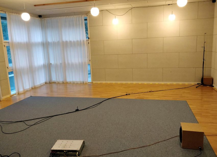
dataset will help the community in benchmarking                   reconstruction for future work, and frame the core chal-
       and comparing state-of-the-art results.                           lenge of this paper as estimation of sound pressure in
                                                                         two-dimensional horizontal planes.
    • We assess the real-world performance of deep                            The function that we seek to reconstruct on this grid
      learning-based sound field magnitude reconstruc-                   is the Fourier transform of the sound field in a frequency
      tion trained on simulated sound fields. For this                   band that covers the low frequencies. The complex-
      purpose, we consider low frequencies, since low-                   valued frequency-domain sound field calculated using the
      frequency room modes can significantly alter lis-                  Fourier transform is given by
      tening experience.Furthermore, we are interested in
      using a very low number of microphones.
                                                                                                    Z
                                                                                         s(r, ω) :=   p(r, t)e−jωt dt           (2)
    • Moreover, we extend the deep learning-based sound                                                   R

      field reconstruction to cover complex-valued inputs,               where ω ∈ R is a given excitation frequency, and p(r, t)
      i.e. both the magnitude and the phase of a sound                   denotes the spatio-temporal sound field with r ∈ R. We
      field. Evaluation is performed in both simulated                   refer to the real and imaginary parts of the sound field
      and real rooms, where a performance gap is ob-                     using sRe (r, ω) and sIm (r, ω), respectively. Note that
      served. We argue why complex sound field recon-                    s is defined as the magnitude of the Fourier transform
      struction may have more difficulties in transferring               in (Lluı́s et al., 2020). Instead, for magnitude recon-
      useful knowledge from synthetic to real data.                      struction, we introduce the magnitude of the sound field
    • Lastly, we demonstrate the application of complex-                                             Z
      valued sound field reconstruction within the field                                |s(r, ω)| :=   p(r, t)e−jωt dt        (3)
      of sound zone control. Specifically, it is shown that                                               R
      sound fields reconstructed from as little as five mi-              for ω ∈ R and r ∈ R.
      crophones pose as valuable inputs to acoustic con-                      The procedure for reconstructing s(r, ω) on Do takes
      trast control.                                                     its starting point from actual observations of the sound
                                                                         field in select positions of the grid. We refer to the col-
    The paper is organized as follows: Section II intro-                 lected set of these available sample points as So , which
duces the concept of sound field reconstruction. Details                 we further define to be a subset of the full grid. That is,
of measurements from real rooms are presented in Sec-                    So ⊆ Do . The cardinality |So | of the set So is the num-
tion III. In Section IV, we focus on the problem of recon-               ber of available sample points, which we will also refer to
structing the magnitude of sound fields, while Section V                 as the number of microphones nmic in later experiments.
extends the model to complex-valued sound fields. Fi-                    We define the samples available to the reconstruction al-
nally, Section VI investigates the application of sound                  gorithm as
zones through sound field reconstruction.                                                      {s(r, ω)}r∈So ⊆Do .               (4)
                                                                              An important aspect of these definitions is that the
II. SOUND FIELD RECONSTRUCTION
                                                                         grid is unitless and positions can be defined in relative
     Our approach towards the sound field reconstruction                 terms. That is, when sampling a point in the grid, only
problem is based on the observation that acoustic pres-                  the relative position within the grid, and hence the room,
sure in a room can be described using a three-dimensional                needs to be known. This allows us to relax the data
regular grid of points defining a three-dimensional dis-                 collection compared to alternative methods that require
crete function. The approach specifically for the purpose                absolute locations. Another important element to con-
of magnitude reconstruction was introduced in (Lluı́s                    sider is that the sampling pattern of So can form any
et al., 2020). First, let R = [0, lx ] × [0, ly ] × [0, lz ] denote      arrangement within Do as long as 1 ≤ |So | ≤ |Do |. As an
a rectangular room, where lx , ly , lz > 0 are the length,               example, this means that sampled points can be irregu-
width, and height of the room, respectively. Given such                  larly distributed spatially in a room.
room, we define the grid as a discrete set of coordinates                     Situations may arise where the sound field resolu-
Do . However, for the sake of simplicity, we reduce the                  tion, as defined by lx , I, ly , and J, is too coarse. As an
three-dimensional problem to a two-dimensional recon-                    example, consider rooms that are either very long, wide,
struction on horizontal planes. The two-dimensional grid                 or in general large. Another example includes applica-
with a constant height zo is defined as                                  tions where fine-grained variations within a sound field
                       n l                                              are of importance. To compensate for this effect, we al-
                             x    ly      o
                                                                         low the reconstruction to base its output on another grid
               Do :=     i     ,j    , zo                         (1)
                           I −1 J −1         i,j                         than Do . Such domain will typically be an upsampling
                                                                         of the original grid, but similarly it can be defined with
for zo ∈ [0, lz ], i = 0, . . . , I − 1, j = 0, . . . , J − 1, and in-   other transformations, e.g. downsampling. Specifically,
tegers I, J ≥ 2. Note, though, that the dataset collected                we define the grid as
for this study, which we will introduce in Section III,
does in fact contain multiple horizontal planes at different                                 n         lx     ly        o
heights. We keep the investigations of three-dimensional                          DoL,P :=        i         ,j      , zo         (5)
                                                                                                      IL − 1 JP − 1        i,j

2     Deep Sound Field Reconstruction in Real Rooms: Introducing the ISOBEL Sound Field Dataset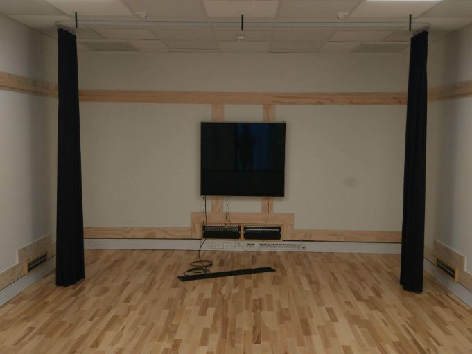
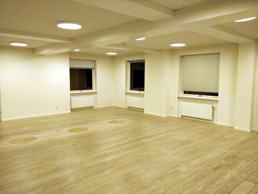
where i = 0, . . . , IL − 1, j = 0, . . . , JP − 1, and L, P                 The dataset consists of measurements from four dif-
must be chosen such that IL, JP ∈ Z+ . Note that a value                ferent rooms as specified in Table I and depicted in Fig. 1.
larger than one for either L or P results in an upsampling              The data collection is an extension to the real room mea-
in the respective dimension.                                            sured in (Lluı́s et al., 2020), which is included in the ISO-
    The task of the sound field reconstruction is then to               BEL Sound Field dataset as Room B for simple access to
estimate the sound field on the grid DoL,P based on the                 all measured rooms. The rooms are located at Aalborg
sampled points So . In particular, the objective of the                 University, Aalborg, Denmark, and Bang & Olufsen a/s,
reconstruction algorithm is to learn parameters w given                 Struer, Denmark. The rooms have significantly different
                                           L,P
                                                                        acoustic properties and also vary in size. Two types of
   gw :       C|So |K          → C|Do |K                    (6)         measurements are conducted in each room: 1) Reverber-
       {s(r, ωk )}r∈So ,ωk ∈Ω 7→ {ŝ(r, ωk )}r∈DoL,P ,ωk ∈Ω             ation time; 2) Sound field. However, only the sound field
                                                                        measurements are released as part of the dataset.
where gw is an estimator and Ω = {ωk }K    k=1 is the set of                 The reverberation times are measured in conformity
frequencies at which the sound field will be reconstructed.             with ISO 3382-2 (ISO 3382-2:2008, 2008) and calculated
The remainder of the paper describes the procedure for                  based on resulting impulse responses using backwards in-
learning parameters w using deep learning-based meth-                   tegration and least-squares best fit evaluation of the de-
ods.                                                                    cay curves.2 The reverberation times reported in the
                                                                        table are the arithmetic averages of 1/3 octave T20 esti-
A. Evaluation Metrics
                                                                        mates in the frequency range 50-316 Hz.
                                                                             The sound field measurements are performed on a
    The successfulness of the estimator is quantitatively               32 by 32 grid with sample points distributed uniformly
judged using normalized mean square error (NMSE) at                     along the length and width of each room. That is, a
each frequency point in {ωk }Kk=1                                       total of 1024 positions are measured in each room if pos-
                                                                        sible, but in some cases it is not feasible to measure all
                           |s(r, ωk ) − ŝ(r, ωk )|2
                     P
                                                                        positions due to e.g. obstacles.3 The horizontal grids
                      r∈DoL,P                                           are measured at four different heights: 1, 1.3, 1.6, and
         NMSEk =                                         .        (7)
                                                                        1.9 meters above the floor.4 This is achieved using the
                                P
                                        |s(r, ωk )|2
                              r∈DoL,P                                   microphone rig depicted in Fig. 1. Two 10 inch loud-
                                                                        speakers are used to acquire sound fields from two dif-
The NMSE provides an average error over all positions in                ferent source positions in each room. Both loudspeakers
the grid between reconstructed and original sound fields                are placed on the floor, one in a corner and one in an
for a single room at a single frequency. We also introduce              arbitrary position. The sound sources are kept in the
an average NMSE, which is the NMSE performance av-                      same position, while the microphones are moved around
eraged over all frequencies of interest as well as over all             the room to record impulse responses. For each micro-
realizations from M trials, e.g. multiple rooms                         phone position in the grid, the two sources play logarith-
                                                                        mic sine sweeps in the frequency range 0.1-24,000 Hz fol-
    MNMSE =
                                                                        lowed by a quiet tail, (Farina, 2000). We use a sampling
                              |sm (r, ωk ) − ŝm (r, ωk )|2
                      P
             K
           M X                                                          frequency of 48,000 Hz. The equipment includes among
     1     X        r∈DoL,P                                             others four G.R.A.S. 40AZ prepolarized free-field micro-
                                P                             .   (8)
    MK    m=1 k=1
                                     |sm (r, ωk )|2                     phones connected to four G.R.A.S. 26CC CCP standard
                           r∈DoL,P                                      preamplifiers and an RME Fireface UFX+ sound card.
                                                                        The four microphones are level calibrated at 1,000 Hz
This measure serves as an overall indication of the ac-                 using a Brüel & Kjær sound calibrator type 4231 prior
curacy of a model, whereas the NMSEk allows a deeper
                                                                        to the measurements.
insight of model behaviors at different frequencies. Note
that the M trials are specific to each experiment and will
be described accordingly.                                               TABLE I. Room characteristics in the ISOBEL Sound Field
                                                                        dataset. The reverberation times are the arithmetic averages
                                                                        of 1/3 octave T20 estimates in the frequency range 50-316Hz.
III. THE ISOBEL SOUND FIELD DATASET

    A major contribution of this paper is the ISOBEL
Sound Field dataset, which is released as open access                   Room                Dim. [m]       Size [m2 /m3 ] T20 [s]
alongside the manuscript.1 The intended purpose is to                   Room B        4.16 x 6.46 x 2.30       27/ 62        0.39
use the measurements from real rooms for evaluation of
                                                                        VR Lab        6.98 x 8.12 x 3.03       57/172        0.37
sound field reconstruction in a diverse set of rooms. Note
that the room-wide measurements of room impulse re-                     List. Room    4.14 x 7.80 x 2.78       32/ 90        0.80
sponses have several other use-cases that will not be fur-              Prod. Room 9.13 x 12.03 x 2.60        110/286        0.77
ther investigated in this paper, but we encourage the use
outside sound field reconstruction as well. This section
details the dataset and the measurement procedure.

Deep Sound Field Reconstruction in Real Rooms: Introducing the ISOBEL Sound Field Dataset                                           3
FIG. 1. Left: Rig with four microphones. Rooms from top left to bottom right: Room B, VR Lab, Listening Room, and
Product Room.
IV. SOUND FIELD MAGNITUDE RECONSTRUCTION cobsen and Juhl, 2013). The function provides a solution
as an infinite summation of room modes in the three di-
In the previous sections we have introduced the prob- mensions of a room, x, y, and z. It is defined as follows
lem of reconstructing sound fields on two-dimensional
grids in rectangular rooms, as well as introduced a real-
world dataset specifically for evaluation of estimators 1 X ψN (r)ψN (r0 )
solving such problem. In recent work, (Lluı́s et al., 2020) G(r, r0 , ω) ≈ − (9)
V (ω/c)2 − (ωN /c)2 − jω/τN
showed that the problem fits within the context of deep N
learning-based methods for image reconstruction. Specif- P P∞ P∞ P∞
where N = nz =0 , for compactness,
ically, the tasks of inpainting, (Bertalmio et al., 2000; Liu nx =0 ny =0
et al., 2018), and super-resolution, (Dong et al., 2016; denotes summation across modal orders in the three di-
Ledig et al., 2017), which can be paralleled to the tasks mensions of the room, and similarly the triplet of inte-
of filling in the grid points that are not measured in the gers (nx , ny , nz ) are represented by N . Furthermore, V
2
sound fields DoL,P \So , as well as upsampling the grid res- denotes the volume of the room, ωN represents angular
olution to achieve fine-grained variations in sound fields. resonance frequency of a mode associated with a specific
One realization is that these methods are designed to N , the shape of the mode is denoted ψN (·), τN is the time
work with real-valued images. To accommodate this, constant of the mode, and c is the speed of sound. As-
(Lluı́s et al., 2020) propose to reconstruct only the mag- suming rigid boundaries, the shape is determined using
nitude of the sound field, i.e. |s(r, ω)|, using a U-Net-like the expression (Jacobsen and Juhl, 2013)
architecture, (Ronneberger et al., 2015). nx πx ny πy nz πz
To this end, the sampled grids are defined as ten- ψN (x) = ΛN cos cos cos . (10)
lx ly lz
sors together with masks specifying which positions
are measured (Lluı́s et al., 2020). As an example, √
Here, ΛN = x y z are constants used for normalization
{|s(r, ωk )|}r∈DoL,P ,k can be constructed as a tensor of the with 0 = 1, 1 = 2 = · · · = 2. Using Sabine’s equation,
form Smag ∈ RIL×JP ×K . The network is trained using a the absorption coefficient is calculated and used to de-
large number of simulated realizations of rooms, as will termine time constants of each mode.This is done by as-
be described in the following section. For the experi- suming that surfaces of a room have uniform distribution
ments, we are interested in assessing the ability of the of absorption.
model to generalize to a wide range of real rooms. In the following experiments, two sets of training
data are used. The first dataset is introduced in (Lluı́s
A. Simulation of Sound Fields for Training Data et al., 2020) and consists of 5,000 rectangular rooms. The
room dimensions are sampled randomly in accordance
Green’s function can be used to approximate sound with the recommendations for listening rooms in ITU-R
fields in rectangular rooms that are lightly damped, (Ja- BS.1116-3 (ITU-R BS.1116-3, 2015). The dataset uses a
4 Deep Sound Field Reconstruction in Real Rooms: Introducing the ISOBEL Sound Field DatasetB. Experiments on the ISOBEL Sound Field Dataset
The U-Net-like architecture has shown promising re-
sults on simulated data and on measurements from a sin-
gle real room (Lluı́s et al., 2020). In the following experi-
ments, we expose the model to the ISOBEL Sound Field
Room B
dataset. We include results from the original model, as
VR Lab well as a model built around a similar architecture but
List. Room using the extended training data with a larger range of
Prod. Room
room dimensions and reverberation characteristics. We
investigate the performance of the model trained with
the two different simulated datasets in the four rooms
included in the real-world dataset. Special attention is
FIG. 2. NMSE in dB of U-Net-based magnitude reconstruc-
paid to the number of available samples, i.e. the number
tion in the four measured rooms with nmic = 15 using the
of microphones nmic . We are mainly interested in set-
original pretrained model presented in (Lluı́s et al., 2020).
tings with a very low number of microphones. In partic-
ular, we show results for 5, 15, and 25 microphones in the
rooms with a total of 32 × 32 = 1024 available positions.
In each room, a total of 40 different and randomly sam-
pled realizations of microphone positions So are used for
each value of nmic . We report the average performance
across the 40 realizations, and use the source located in
one of the corners of each room.
Fig. 2 and Fig. 3 show NMSEk results for 15 mi-
crophones of model trained with the original and the
extended datasets, respectively. It is clear that the
model trained with the original dataset does not gener-
alize well to all the rooms. This behavior is expected,
Room B
since the training data are not designed to represent
VR Lab
List. Room rooms that fall outside the recommendations for listening
Prod. Room room dimensions. On the contrary, the extended training
data are motivated in encompassing a wider selection of
rooms, which also shows in the results for e.g. the Prod-
uct Room. One important observation in this regard is
FIG. 3. NMSE in dB of U-Net-based magnitude reconstruc- that performance does not decrease in rooms that are
tion in the four measured rooms with nmic = 15 using the already represented in the simulated data when more di-
model presented in (Lluı́s et al., 2020) trained using the ex- verse simulated rooms are included, which can e.g. be
tended dataset. seen from the performance in Room B. This result in-
dicates that the capacity of the model is sufficient for
generalizing to a wide range of diverse rooms and room
constant reverberation time T60 of 0.6 s and only includes
room modes in the x and y dimensions, i.e. nz = 0.
The second dataset consists of 20,000 rectangular TABLE II. MNMSE in dB with M = 40 different and ran-
rooms. Room dimensions are uniformly sampled with domly sampled realizations of So for each room in the ISOBEL
V ∼ U(50, 300)m3 , lx ∼ U(3.5, 10)m, lz ∼ U(1.5, 3.5)m, SF dataset. A lower score is better.
and ly = V /lx lz . Compared to the first dataset, the room
dimensions span a larger range and allow us to represent nmic
e.g. the Product Room, which is not included in the orig-
Room Model 5 15 25
inal training data. The dataset uses reverberation times
T60 sampled from U(0.2, 1.0)s and includes room modes Orig. -6.33 -8.71 -9.62
in all three x-, y-, and z-dimensions. Room B
Ext. -6.27 -8.84 -10.25
For both datasets, a grid DoL,P is defined with I =
J = 8 and L = P = 4, which effectively divides a sound Orig. -4.01 -5.08 -5.63
VR Lab
field into 32x32 uniformly-spaced microphone positions. Ext. -4.12 -6.78 -8.05
Using this grid, the magnitude of the sound field is re- Orig. -4.38 -6.92 -7.94
constructed at 1/12 octave center-frequencies resolution List. Room
Ext. -5.00 -7.61 -8.44
in the range [30, 300] Hz. Simulations are specified to
include all room modes with a resonance frequency be- Orig. -3.89 -4.91 -5.55
Prod. Room
low 400 Hz, which means that there is a total of K = 40 Ext. -5.18 -6.67 -7.73
frequency slices.
Deep Sound Field Reconstruction in Real Rooms: Introducing the ISOBEL Sound Field Dataset 5Encoder Decoder
1024 1024
2
512 512 1536 1536 512 512
4
4
4
256 256 768 768 256 256
8
8
8
16
16
16
128128 384 384 128128
PConv 5x5 PConv 3x3 Upsample 2x2 Skip/concat
32
32
32
80 80 208 208 80 80
SM Ŝ
FIG. 4. Architecture of the U-Net-like convolutional neural network proposed for complex sound field reconstruction. S is the
tensor with real and imaginary sound fields concatenated along the frequency-dimension, M is the mask tensor, and Ŝ is the
reconstructed sound field tensor.
acoustic characteristics, given that the model is provided the sound fields such that the U-Net-based model re-
with ample training samples. ceives real-valued inputs. Specifically, we present the
Table II details MNMSE results, which are the model to real and imaginary parts of sound fields sep-
NMSE results averaged across frequencies K = 40 and So arately. That is, where the magnitude-based model re-
realizations M = 40. The MNMSE results for nmic = 15 ceive as input {|s(r, ωk )|}r∈DoL,P ,k in the tensor form
are the condensed results shown for the NMSEk in Figs. 2 Smag ∈ RIL×JP ×K , the complex-based model in-
and 3. The scores in the table reiterate the observa- stead receives a concatenation of the real and imagi-
tions from the figures, performance is improved with nary sound fields. Specifically, using the real sound
the extended training data for some rooms in particu- field {sRe (r, ωk )}r∈DoL,P ,k with the tensor form SRe ∈
lar, while performance is maintained in the other rooms.
RIL×JP ×K , and similarly the imaginary sound field ten-
Interestingly, there seems to be a tendency of more pro-
sor SIm ∈ RIL×JP ×K , we define the concatenated input:
nounced improvements with a larger number of micro-
phones. We attribute this effect to similar observations
S := [SRe SIm ] , (11)
within classical methods that as the number of micro-
IL×JP ×2K
phones increase, relative improvement for reconstruction where S ∈ R is the resulting tensor with
is higher at low frequencies as opposed to the high- real and imaginary sound fields concatenated along the
frequency range, (Ajdler et al., 2006; Lluı́s et al., 2020). frequency-dimension. Note that the complex-valued
In summary, the deep learning-based model is con- sound field is easily recovered from this tensor form. In
firmed to possess the ability to generalize to a diverse addition, we define a mask tensor M ∈ RIL×JP ×2K com-
set of real rooms for sound field magnitude reconstruc- puted from So and DoL,P .
tion. Based solely on training with simulated data, these We follow the pre- and postprocessing steps as de-
promising results motivate further investigations, e.g. of scribed in (Lluı́s et al., 2020), which entails comple-
reconstructing the complex-valued sound fields. tion, scaling, upsampling, mask generation, and rescal-
ing based on linear regression. These steps are, however,
adjusted such that they operate on a tensor that has
V. COMPLEX SOUND FIELD RECONSTRUCTION doubled in size from K to 2K in the third dimension.
We propose to extend the U-Net-based model Furthermore, we have observed significant improvements
to work with complex-valued room transfer functions by changing the min-max scaling of the input to a max
(RTFs). Reconstruction of both magnitude and phase scaling that takes into account both real and imaginary
of sound fields enable new opportunities, such as the ap- parts for each frequency slice. Specifically:
plication of sound zones. A topic, which we investigate sRe (r, ωk )
in Section VI. sRe,s (r, ωk ) := (12)
maxr∈So (|sRe (r, ωk )|, |sIm (r, ωk )|)
The proposed model is based on the model de-
signed to work with the magnitude of sound fields.
Note that deep learning-based models that work di- sIm (r, ωk )
sIm,s (r, ωk ) := (13)
rectly on complex-valued inputs have been introduced, maxr∈So (|sRe (r, ωk )|, |sIm (r, ωk )|)
e.g. within Transformers (Kim et al., 2020; Yang et al.,
for each ωk . Note that this alters the scaling operation
2020), but in this paper we instead choose to process
from working in the range [0,1] to working in [-1,1]. The
6 Deep Sound Field Reconstruction in Real Rooms: Introducing the ISOBEL Sound Field Datasetmotivation in doing so, is that values can be negative, in
contrast to the real values from the magnitude. By using
max scaling we ensure that zero will not shift between
realizations.
The architecture of the proposed neural network, as
illustrated in Fig. 4, is based on a U-Net (Ronneberger
et al., 2015). We employ partial convolutions (PConv) as
proposed for image inpainting in (Liu et al., 2018). In the
encoding part of the U-Net, we use a stride of two in the
partial convolutions in order to halve the feature maps,
while doubling the number of kernels in each layer. The
decoder part acts opposite with upsampling feature maps
and reducing the number of kernels to reach an output FIG. 5. NMSE in dB for complex reconstruction of simulated
tensor Ŝ with matching dimensions to the input tensor sound fields in the test set with 190 different rooms and three
S. We use ReLU as activation function in the encoding realizations of So in each room (M = 570 for each value of
part, and leaky ReLU with a slope coefficient of -0.2 in nmic ). The solid lines indicate average NMSEk shown with
the decoder. We initialize the weights using the uniform 95% confidence intervals. Colors indicate different values of
Xavier method (Glorot and Bengio, 2010), initialize the nmic in the range [5, 55].
biases as zero, and use the Adam optimizer (Kingma and
Ba, 2014) with early stopping when performance on a val-
idation set stops increasing. Due to the increased input
and output sizes, we double the number of kernels in all
layers compared to the U-Net for magnitude reconstruc-
tion. We also do not use a 1x1 convolution with sigmoid
activation in the last layer, since the range of our output
is not constrained to [0,1] but instead [-1,1]. We have
not experienced any decreases in performance from not
including this layer.
Room B
VR Lab
A. Experiments
List. Room
Prod. Room
In this section, we assess the complex-valued sound
field reconstruction. The simulated extended dataset in-
troduced in Section IV A is used to train the model. It
is important to note that NMSE scores are not directly FIG. 6. Average NMSEk in dB of complex reconstruction in
comparable between magnitude and complex reconstruc- the four measured rooms with nmic = 15.
tion, for which reason it is not possible to scrutinize dif-
ferences between the two types of models. That is, the
results presented in the following experiments will stand
on their own, and only indicative parallels can be drawn formances in the real rooms are not comparable to those
to the results from magnitude reconstruction. from simulated data. Moreover, although it is not pos-
First, we test how the model performs on the sim- sible to compare directly, performance seems worse than
what is achieved with the magnitude-based reconstruc-
ulated data associated with the training data, but held
tion in the same rooms, see Fig. 3. That is, the complex
out specifically for evaluation. This test set consists of
reconstruction model is not transferring useful knowledge
190 simulated rooms, the validation set contains approx-
as successfully from the simulations-based training to the
imately 1,000 rooms, and the training set holds the re-
real world. Given that the network is able to reconstruct
maining rooms from the 20,000 available rooms. In each
the simulated sound fields, it appears that the complex
room, three different realizations of So are used for each
simulation model is a worse match for the real rooms than
value of nmic . Results in terms of NMSE are shown in
the magnitude simulation model. The outcome is that
Fig. 5. Some tendencies are similar to those observed
the framework is able to reconstruct sound fields which
for magnitude reconstruction, such as improvements in
performance with an increasing number of available mi- are close to fields included in the training data, it is indi-
crophones. At the same time, as frequency increases, cated that the complex simulations are a poor match for
performance degrades. the real rooms. Two apparent differences are the iden-
Next, we evaluate the complex reconstruction model tical boundary conditions at all surfaces and perfectly
on the ISOBEL Sound Field dataset. The approach is rectangular geometry assumed in the simulations, but
similar to the experiment in Section IV B, except the use which are not true in the real rooms. To provide insights
of the complex-valued sound fields instead of the mag- into how the network behaves relative to rooms which
nitude. As can be seen from the results in Fig. 6, per- does not match the training data set we now present the
following simulations.
Deep Sound Field Reconstruction in Real Rooms: Introducing the ISOBEL Sound Field Dataset 7Simulated Simulated Simulated
Test→
List. Room List. Room List. Room
Train↓
lx + U(−0.25, 0.25)m lx + U(−1.0, 1.0)m
Simulated
List. Room
Simulated
List. Room
lx + U(−0.25, 0.25)m
Simulated
List. Room
lx + U(−1.0, 1.0)m
FIG. 7. NMSE in dB for complex reconstruction of simulated sound fields in rooms with no or small variations in the room
dimensions. Rows: Training data. Columns: Test data. Four random realizations of So are used in each of the 11 test rooms
(M = 44). The solid lines indicate average NMSEk shown with 95% confidence intervals. Colors indicate different nmic values,
i.e., nmic = 5 (blue), nmic = 15 (orange), nmic = 25 (green), nmic = 35 (red), nmic = 45 (purple), and nmic = 55 (brown).
B. Discussion of Experiments with small variations of the 0.25 m scale, performance
rapidly degrades with increasing frequency. On the di-
Several optimizations and fine-tuning approaches agonal, training data match test data, and once again
have been investigated for the complex reconstruction high frequencies see a significant performance decrease
in real rooms without achieving notable improvements. with increasing uncertainty. In general, the models do
Instead, we take another approach, and show what hap- not perform well on datasets with more variation than
pens to the model, when it is exposed to data that are not what is included in their own training data, which can
represented in the training data. To this end, we are in- be seen in the three upper right figures.
terested in assessing the performance of room specialized Further experiments showed that the three models
models. That is, if room dimensions and reverberation do not generalize to the real-world measurements of the
time are known, how well will a model trained specifi- Listening Room. This result indicates that the simplifi-
cally for that room perform. For this, we introduce new cations imposed during the simulations of rooms causes
datasets each with 824 realizations for training, 165 for the simulated sound fields to not represent the exact real
validation, and 11 for testing. Each simulated realiza- rooms we intend it to. That is, a model trained with
tion has a randomly positioned source. In total, three simulated data generated using exact parameters of a
such datasets are generated according to the procedure real room will not be able to reconstruct the sound field
described in Section IV A. The first dataset assumes that accurately in the real room. As suggested by our results,
room characteristics are known perfectly, we use the pa- neither will a model trained with ±1 m uncertainty. This
rameters of the Listening Room. The second and third calls for inclusion of diverse room parameters when train-
datasets introduce uncertainty in the room dimensions. ing a model with simulated data if the intended purpose
In particular, we alter the length and width of rooms, is to use the reconstruction in real rooms.
while keeping the aspect ratio (lx /ly ) of the room con- We showed in Section IV how magnitude reconstruc-
stant. We accomplish this by uniformly sampling an er- tion recovered performance in some of the real rooms
ror, which is added to the length of a room, and cor- by using an extended training dataset with more diverse
rect the width to achieve the original aspect ratio. The simulated rooms. The same effect is not observed for
two datasets sample errors in the range [-0.25, 0.25] m complex reconstruction. We believe two factors are the
and [-1, 1] m, respectively. The results for the three main reasons: 1) the boundary conditions in the simu-
models evaluated on each of the test sets are shown in lations assume nearly rigid walls and do not include e.g.
Fig. 7. The first column shows how the three models per- phase shifts of real wall reflections; 2) the simulations
form on the dataset with no added uncertainties. Even assume perfectly rectangular rooms with a uniform dis-
8 Deep Sound Field Reconstruction in Real Rooms: Introducing the ISOBEL Sound Field Datasettribution of absorption. Thus, we hypothesize that the Here, the sound pressure observed at the physical micro-
model does not see representative data during training, phone locations are modeled as a combination of imping-
analogous to not having the correct room dimensions rep- ing plane waves
resented in the training data.
s(r1 , ω) φ1 (r1 ) · · · φN (r1 ) b1 (ω)
.. .
= . .. .. .
. (16)
VI. THE SOUND ZONES APPLICATION
. . . . .
One potential application for the sound field recon- s(rM , ω) φ1 (rM ) · · · φN (rM ) bN (ω)
struction presented in this paper, is in the process of set- | {z } | {z
Φ
}| {z }
s(ω) b(ω)
ting up sound zones. Sound zones generally refers to the
scenario where multiple loudspeakers are used to repro- T
where s(·, ·) is defined in (2), φn (rm ) = ejkn rm is the
duce individual audio signals to individual people within
candidate plane wave, propagating with wave number
a room (Betlehem et al., 2015). To control the sound
kn ∈ R3 , to observation point rm ∈ R3 , and bn (ω) ∈ C is
field at the location of the listeners in the room, it is nec-
the complex weight of the nth candidate plane wave. The
essary to know the RTFs between each loudspeaker and
candidate plane waves can be obtained by sampling the
locations sampling the listening regions. If the desired lo-
wave number domain in a cubic grid. Note that the eigen-
cations of the sound zones change over time, it becomes
functions of the room used in Green’s function can be ex-
labor intensive to measure all the RTFs in situ. As an
panded into a number of plane waves whose propagation
alternative, a small set of RTFs could be measured and
directions in the wave number domain equals the charac-
used to extrapolate the RTFs at the positions of interest.
teristic frequency of the eigenfunction (kkn k22 = (ω/c)2 ).
This fact was used in (Fernandez-Grande, 2019) to reg-
1. Setup ularize the sparse reconstruction problem as
For this example, we will explore the scenario where
sound is reproduced in one zone (the bright zone) and min ks(ω) − Φb(ω)k2 + λkL(ω)b(ω)k1 (17)
b(ω)
suppressed in another zone (the dark zone).5
The question posed in a sound zones scenario, is how where λ ∈ R+ and L(ω) ∈ RN ×N is a diagonal matrix,
the output of the available loudspeakers should be ad- where the diagonal elements express the distance between
justed to achieve the desired scenario. A simple formula- the characteristic frequency associated with the nth can-
tion of this problem in the frequency domain is typically didate plane wave and the angular excitation frequency
denoted acoustic contrast control and relies on maximiz- ω as |kkN k22 − (ω/c)2 |.
ing the ratio of mean square pressure in the bright zone Note that the sparse reconstruction model is not di-
relative to the dark zone (Choi and Kim, 2002). This rectly comparable to the proposed sound field reconstruc-
ratio is termed as the acoustic contrast and can be ex- tion. This is due to the sparse reconstruction relying on
pressed as knowledge of the absolute locations of the microphone ob-
servations. The proposed algorithm, on the other hand,
kHB (ω)q(ω)k22 only requires the relative microphone locations on a unit-
Contrast(ω) := (14)
kHD (ω)q(ω)k22 less observation grid.
where HB (ω) ∈ CM ×L is a matrix of RTFs from L loud- 3. Experiments
speakers to M microphone positions in the bright zone
and HD (ω) ∈ CM ×L are the RTFs from the loudspeak- For the experiments, we use the simulated Listening
ers to points in the dark zone. The adjustment of the Room from the previous section, with eight loudspeakers
loudspeaker responses q(ω) ∈ CL can be determined as placed at the corners of the floor and halfway between
the eigenvector of (HH −1 H the corners. We have two predefined zones in the middle
D (ω)HD (ω)+λD I) HB (ω)HB (ω)
which corresponds to the maximal eigenvalue (Elliott of the room, which are bright and dark zone respectively.
et al., 2012), where ·H denotes the Hermitian transpose. We now, sample random positions in the 32 by 32 x,y-
In this investigation, the regularization parameter is cho- grid 1 m above the floor and use those observations to
sen as estimate the RTFs within the zones.
We compare the sparse reconstruction method to the
λD = 0.01kHH D (ω)HD (ω)k2 . (15)
deep learning-based model trained in the previous sec-
This choice is made to scale the regularization relative tion. Specifically, the room specialized models are used.
to the maximal singular value of HH The resulting performance is evaluated in terms of
D (ω)HD (ω), thereby,
controlling the condition number of the inverted matrix. the acoustic contrast over 50 random microphone sam-
plings for each number of microphones. In Fig. 8 the
results are based on evaluations using the true RTFs
2. Sparse Reconstruction method
when the loudspeaker weights are determined using ei-
An alternative method for estimating the RTFs at ther the true RTFs, estimated RTFs based on the model
positions of interest can be obtained by a sparse recon- trained with simulated room with no added uncertain-
struction problem inspired by (Fernandez-Grande, 2019). ties, or estimates based on the sparse reconstruction. It
Deep Sound Field Reconstruction in Real Rooms: Introducing the ISOBEL Sound Field Dataset 930 30
Contrast [dB]
Contrast [dB]
20 20
10 10
0 0
-10 -10
50 100 200 50 100 200
Frequency [Hz] Frequency [Hz]
(a) (a)
30 30
Contrast [dB]
Contrast [dB]
20 20
10 10
0 0
-10 -10
50 100 200 50 100 200
Frequency [Hz] Frequency [Hz]
(b) (b)
FIG. 8. Contrast results for the dataset with no added uncer- FIG. 9. Contrast results for the simulated Listening Room
tainty to the simulated Listening Room (50 different obser- with lx + U(−1.0, 1.0) m (50 different observation masks).
vation masks). (blue): Perfectly known TFs. (black): Deep (blue): Perfectly known TFs. (black): Deep learning model.
learning model. (red): Sparse reconstruction. (dashed): ±1 (red): Sparse reconstruction. (dashed): ±1 standard devia-
standard deviation. tion.
is observed that the deep learning-based model performs surements from real rooms, which are released alongside
better than the sparse reconstruction below 150 Hz for 5 the paper. The focus of the work is threefold: exam-
and 15 microphones. Above 150 Hz, both models strug- ine performance of simulation-based learning of magni-
gle to provide sufficiently accurate RTFs to create sound tude reconstruction in real rooms, extend reconstruction
zones. to complex-valued sound fields, and show a sound zone
In Fig. 9, the model specialized for the Listening application taking advantage of the reconstructed sound
Room with lx +U(−1.0, 1.0) m, is compared to the sparse fields. Experiments for each of the three directions indi-
reconstruction. As expected, the resulting performance cate promising aspects of data-driven sound field recon-
is reduced for the model. However, it is observed that struction, even with a low number of arbitrarily placed
there is still a benefit when using 5 microphones. At microphones.
15 microphones, on the other hand, the performance is In the future, it would be of interest to investigate
comparable for both methods. whether transfer learning can help bridge the discrep-
These results indicate that sound zones could be cre- ancies between simulated and real data. With the ad-
ated based on sound fields extrapolated from very few dition of more rooms, some could be used in the train-
microphone positions. However, at this stage it requires ing phase. Furthermore, three-dimensional reconstruc-
models which are specialized to the particular room or tion can be achieved using available convolutional models
a narrow range of rooms. Alternatively, it would be re- designed specifically to solve three-dimensional problems.
quired to increase the number of microphones to improve
the accuracy of the estimated RTFs. ACKNOWLEDGMENTS
VII. CONCLUSION This work is part of the ISOBEL Grand Solutions
project, and is supported in part by the Innovation Fund
In this paper, deep learning-based sound field recon- Denmark (IFD) under File No. 9069-00038A.
struction is evaluated using a new set of extensive mea-
10 Deep Sound Field Reconstruction in Real Rooms: Introducing the ISOBEL Sound Field Dataset1 The data are collected under the Interactive Sound Zones for Bet- Kim, J., El-Khamy, M., and Lee, J. (2020). “T-GSA: Trans-
ter Living (ISOBEL) project, which aims to develop interactive former with Gaussian-Weighted Self-Attention for Speech En-
sound zone systems, responding to the need for sound exposure hancement,” in ICASSP 2020 - 2020 IEEE International Con-
control in dynamic real-world contexts, adapted to and tested in ference on Acoustics, Speech and Signal Processing (ICASSP),
healthcare and homes. The ISOBEL Sound Field dataset can be pp. 6649–6653, doi: 10.1109/ICASSP40776.2020.9053591.
accessed at https://doi.org/10.5281/zenodo.4501339. Kingma, D. P., and Ba, J. (2014). “Adam: A Method for Stochas-
2 Further details of the experimental setup and protocol, e.g. equip- tic Optimization,” arXiv:1412.6980 [cs] .
ment, are available in the measurement reports included with the Ledig, C., Theis, L., Huszar, F., Caballero, J., Cunningham, A.,
dataset. Acosta, A., Aitken, A., Tejani, A., Totz, J., Wang, Z., and Shi,
3 See footnote 2.
W. (2017). “Photo-realistic single image super-resolution using a
generative adversarial network,” in Proceedings of the IEEE Con-
4 Room B has measurements at a single height: 1 meter above the ference on Computer Vision and Pattern Recognition (CVPR).
floor. Liu, G., Reda, F. A., Shih, K. J., Wang, T.-C., Tao, A., and Catan-
5 Theuse case with multiple individual audio signals can be realized zaro, B. (2018). “Image Inpainting for Irregular Holes Using Par-
using superposition of this solution and one where the role of bright tial Convolutions,” in Computer Vision – ECCV 2018, edited by
and dark zone are reversed. V. Ferrari, M. Hebert, C. Sminchisescu, and Y. Weiss, Lecture
Notes in Computer Science, Springer International Publishing,
Ajdler, T., Sbaiz, L., and Vetterli, M. (2006). “The Plenacoustic Cham, pp. 89–105, doi: 10.1007/978-3-030-01252-6_6.
Function and Its Sampling,” IEEE Transactions on Signal Pro- Lluı́s, F., Martı́nez-Nuevo, P., Møller, M. B., and Shepstone, S. E.
cessing 54(10), 3790–3804, doi: 10.1109/TSP.2006.879280. (2020). “Sound field reconstruction in rooms: Inpainting meets
Antonello, N., Sena, E. D., Moonen, M., Naylor, P. A., and van super-resolution,” The Journal of the Acoustical Society of Amer-
Waterschoot, T. (2017). “Room Impulse Response Interpolation ica 148(2), 649–659, doi: 10.1121/10.0001687.
Using a Sparse Spatio-Temporal Representation of the Sound Mignot, R., Chardon, G., and Daudet, L. (2014). “Low Fre-
Field,” IEEE/ACM Transactions on Audio, Speech, and Lan- quency Interpolation of Room Impulse Responses Using Com-
guage Processing 25(10), 1929–1941, doi: 10.1109/TASLP.2017. pressed Sensing,” IEEE/ACM Transactions on Audio, Speech,
2730284. and Language Processing 22(1), 205–216, doi: 10.1109/TASLP.
Bertalmio, M., Sapiro, G., Caselles, V., and Ballester, C. (2000). 2013.2286922.
“Image inpainting,” in Proceedings of the 27th Annual Confer- Møller, M. B., and Østergaard, J. (2020). “A Moving Hori-
ence on Computer Graphics and Interactive Techniques, SIG- zon Framework for Sound Zones,” IEEE/ACM Transactions
GRAPH ’00, ACM Press/Addison-Wesley Publishing Co., USA, on Audio, Speech, and Language Processing 28, 256–265, doi:
pp. 417–424, doi: 10.1145/344779.344972. 10.1109/TASLP.2019.2951995.
Betlehem, T., Zhang, W., Poletti, M. A., and Abhayapala, T. D. Nowakowski, T., de Rosny, J., and Daudet, L. (2017). “Robust
(2015). “Personal Sound Zones: Delivering interface-free audio source localization from wavefield separation including prior in-
to multiple listeners,” IEEE Signal Processing Magazine 32(2), formation,” The Journal of the Acoustical Society of America
81–91, doi: 10.1109/MSP.2014.2360707. 141(4), 2375–2386, doi: 10.1121/1.4979258.
Cecchi, S., Carini, A., and Spors, S. (2018). “Room Response Radlovic, B. D., Williamson, R. C., and Kennedy, R. A. (2000).
Equalization—A Review,” Applied Sciences 8(1), 16, doi: 10. “Equalization in an acoustic reverberant environment: Robust-
3390/app8010016. ness results,” IEEE Transactions on Speech and Audio Process-
Choi, J., and Kim, Y. (2002). “Generation of an acoustically bright ing 8(3), 311–319, doi: 10.1109/89.841213.
zone with an illuminated region using multiple sources,” Journal Ronneberger, O., Fischer, P., and Brox, T. (2015). “U-Net: Con-
of the Acoustical Society of America 111(4), 1695–1700. volutional Networks for Biomedical Image Segmentation,” in
Dong, C., Loy, C. C., He, K., and Tang, X. (2016). “Image Super- Medical Image Computing and Computer-Assisted Intervention
Resolution Using Deep Convolutional Networks,” IEEE Transac- – MICCAI 2015, edited by N. Navab, J. Hornegger, W. M.
tions on Pattern Analysis and Machine Intelligence 38(2), 295– Wells, and A. F. Frangi, Lecture Notes in Computer Science,
307, doi: 10.1109/TPAMI.2015.2439281. Springer International Publishing, Cham, pp. 234–241, doi:
Elliott, S. J., Cheer, J., Choi, J., and Kim, Y. (2012). “Robustness 10.1007/978-3-319-24574-4_28.
and regularization of personal audio systems,” IEEE Transac- Tylka, J. G., and Choueiri, E. (2015). “Comparison of techniques
tions on Audio, Speech, and Language Processing 20(7), 2123– for binaural navigation of higher-order ambisonic soundfields,”
2133. in Audio Engineering Society Convention 139.
Farina, A. (2000). “Simultaneous Measurement of Impulse Re- Verburg, S. A., and Fernandez-Grande, E. (2018). “Reconstruction
sponse and Distortion with a Swept-Sine Technique,” in Pro- of the sound field in a room using compressive sensing,” The
ceedings of the Audio Engineering Society Convention 108. Journal of the Acoustical Society of America 143(6), 3770–3779,
Fernandez-Grande, E. (2019). “Sound field reconstruction in a doi: 10.1121/1.5042247.
room from spatially distributed measurements,” in 23rd Inter- Vu, T. P., and Lissek, H. (2020). “Low frequency sound field recon-
national Congress on Acoustics, pp. 4961–68. struction in a non-rectangular room using a small number of mi-
Genovese, A. F., Gamper, H., Pulkki, V., Raghuvanshi, N., and Ta- crophones,” Acta Acustica 4(2), 5, doi: 10.1051/aacus/2020006.
shev, I. J. (2019). “Blind Room Volume Estimation from Single- Yang, M., Ma, M. Q., Li, D., Tsai, Y. H., and Salakhutdinov,
channel Noisy Speech,” in ICASSP 2019 - 2019 IEEE Interna- R. (2020). “Complex Transformer: A Framework for Modeling
tional Conference on Acoustics, Speech and Signal Processing Complex-Valued Sequence,” in ICASSP 2020 - 2020 IEEE In-
(ICASSP), pp. 231–235, doi: 10.1109/ICASSP.2019.8682951. ternational Conference on Acoustics, Speech and Signal Process-
Glorot, X., and Bengio, Y. (2010). “Understanding the difficulty ing (ICASSP), pp. 4232–4236, doi: 10.1109/ICASSP40776.2020.
of training deep feedforward neural networks,” in Proceedings 9054008.
of the Thirteenth International Conference on Artificial Intelli- Yu, W., and Kleijn, W. B. (2021). “Room Acoustical Parame-
gence and Statistics, pp. 249–256. ter Estimation From Room Impulse Responses Using Deep Neu-
ISO 3382-2:2008 (2008). “Acoustics — Measurement of room ral Networks,” IEEE/ACM Transactions on Audio, Speech, and
acoustic parameters — Part 2: Reverberation time in ordinary Language Processing 29, 436–447, doi: 10.1109/TASLP.2020.
rooms,” Standard. 3043115.
ITU-R BS.1116-3 (2015). “Methods for the subjective assessment
of small impairments in audio systems,” Standard.
Jacobsen, F., and Juhl, P. M. (2013). Fundamentals of General
Linear Acoustics (John Wiley & Sons).
Karjalainen, M., Makivirta, A., Antsalo, P., and Valimaki, V.
(2001). “Low-frequency modal equalization of loudspeaker-room
responses,” in Audio Engineering Society Convention 111.
Deep Sound Field Reconstruction in Real Rooms: Introducing the ISOBEL Sound Field Dataset 11You can also read