A Futuristic Least-cost Optimisation Model of CO2 Transportation and Storage in the UK/UK Continental Shelf (UKCS) - DEPARTMENT OF ECONOMICS ...
←
→
Page content transcription
If your browser does not render page correctly, please read the page content below
NORTH SEA STUDY OCCASIONAL PAPER
                    No. 112

 A Futuristic Least-cost Optimisation Model of CO2
      Transportation and Storage in the UK/UK
                Continental Shelf (UKCS)

                Professor Alexander G. Kemp and
                          Dr Sola Kasim

March, 2009                                       Price £25.00

              DEPARTMENT OF ECONOMICS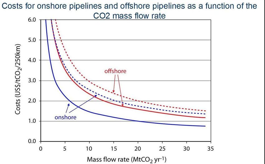
ISSN 0143-022X

                               NORTH SEA ECONOMICS

Research in North Sea Economics has been conducted in the Economics Department since
1973. The present and likely future effects of oil and gas developments on the Scottish
economy formed the subject of a long term study undertaken for the Scottish Office. The
final report of this study, The Economic Impact of North Sea Oil on Scotland, was published
by HMSO in 1978. In more recent years further work has been done on the impact of oil on
local economies and on the barriers to entry and characteristics of the supply companies in
the offshore oil industry.

The second and longer lasting theme of research has been an analysis of licensing and fiscal
regimes applied to petroleum exploitation. Work in this field was initially financed by a
major firm of accountants, by British Petroleum, and subsequently by the Shell Grants
Committee. Much of this work has involved analysis of fiscal systems in other oil producing
countries including Australia, Canada, the United States, Indonesia, Egypt, Nigeria and
Malaysia. Because of the continuing interest in the UK fiscal system many papers have been
produced on the effects of this regime.

From 1985 to 1987 the Economic and Social Science Research Council financed research on
the relationship between oil companies and Governments in the UK, Norway, Denmark and
The Netherlands. A main part of this work involved the construction of Monte Carlo
simulation models which have been employed to measure the extents to which fiscal systems
share in exploration and development risks.

Over the last few years the research has examined the many evolving economic issues
generally relating to petroleum investment and related fiscal and regulatory matters. Subjects
researched include the economics of incremental investments in mature oil fields, economic
aspects of the CRINE initiative, economics of gas developments and contracts in the new
market situation, economic and tax aspects of tariffing, economics of infrastructure cost
sharing, the effects of comparative petroleum fiscal systems on incentives to develop fields
and undertake new exploration, the oil price responsiveness of the UK petroleum tax system,
and the economics of decommissioning, mothballing and re-use of facilities. This work has
been financed by a group of oil companies and Scottish Enterprise, Energy. The work on
CO2 Capture, EOR and storage is also financed by a grant from the Natural Environmental
Research Council (NERC).

For 2009 the programme examines the following subjects:

       a) Effects of Requirements on Investors in UKCS to purchase CO2 allowances
       relating to emissions from 2013 under the EU ETS
       b) Least-Cost Transportation Network for CO2 in UK/UKCS
       c) Comparative study of Petroleum Taxation in North West Europe/ North Atlantic
               (UK, Norway, Denmark, Netherlands, Ireland, Faroe Islands, Iceland and
               Greenland)
       d) Economics of Decommissioning in the UKCS: Further Analysis
       e) Economics of Gas Exploitation from West of Shetland

                                                                                             i
f) Prospective Activity levels in the UKCS to 2035
g) EOR from CO2 Injection
h) General Financial Incentives for CCS in UK
The authors are solely responsible for the work undertaken and views expressed. The
sponsors are not committed to any of the opinions emanating from the studies.
Papers are available from:
The Secretary (NSO Papers)
University of Aberdeen Business School
Edward Wright Building
Dunbar Street
Aberdeen A24 3QY
Tel No: (01224) 273427
Fax No: (01224) 272181
Email: a.g.kemp@abdn.ac.uk
Recent papers published are:
OP 98 Prospects for Activity Levels in the UKCS to 2030: the 2005
Perspective
By A G Kemp and Linda Stephen (May 2005), pp. 52 £20.00
OP 99 A Longitudinal Study of Fallow Dynamics in the UKCS
By A G Kemp and Sola Kasim, (September 2005), pp. 42 £20.00
OP 100 Options for Exploiting Gas from West of Scotland
By A G Kemp and Linda Stephen, (December 2005), pp. 70 £20.00
OP 101 Prospects for Activity Levels in the UKCS to 2035 after the
2006 Budget
By A G Kemp and Linda Stephen, (April 2006) pp. 61 £30.00
OP 102 Developing a Supply Curve for CO2 Capture, Sequestration and
EOR in the UKCS: an Optimised Least-Cost Analytical
Framework
By A G Kemp and Sola Kasim, (May 2006) pp. 39 £20.00
OP 103 Financial Liability for Decommissioning in the UKCS: the
Comparative Effects of LOCs, Surety Bonds and Trust Funds
By A G Kemp and Linda Stephen, (October 2006) pp. 150 £25.00
OP 104 Prospects for UK Oil and Gas Import Dependence £25.00
By A G Kemp and Linda Stephen, (November 2006) pp. 38
OP 105 Long-term Option Contracts for Carbon Emissions
By A G Kemp and J Swierzbinski, (April 2007) pp. 24 £25.00
iiOP 106 The Prospects for Activity in the UKCS to 2035: the 2007
Perspective
By A G Kemp and Linda Stephen (July 2007) pp.56 £25.00
OP 107 A Least-cost Optimisation Model for CO2 capture
By A G Kemp and Sola Kasim (August 2007) pp.65 £25.00
OP 108 The Long Term Structure of the Taxation System for the UK
Continental Shelf £25.00
By A G Kemp and Linda Stephen (October 2007) pp.116
OP 109 The Prospects for Activity in the UKCS to 2035: the 2008
Perspective £25.00
By A G Kemp and Linda Stephen (October 2008) pp.67
OP 110 The Economics of PRT Redetermination for Incremental £25.00
Projects in the UKCS
By A G Kemp and Linda Stephen (November 2008) pp. 56
OP 111 Incentivising Investment in the UKCS: a Response to £25.00
Supporting Investment: a Consultation on the North Sea Fiscal
Regime
By A G Kemp and Linda Stephen (February 2009) pp.93
OP 112 A Futuristic Least-cost Optimisation Model of CO2 £25.00
Transportation and Storage in the UK/ UK Continental Shelf
By A G Kemp and Dr Sola Kasim (March 2009) pp.53
iiiA Futuristic Least-cost Optimisation Model of CO2 Transportation and Storage
in the UK/UK Continental Shelf (UKCS)
Professor Alexander G. Kemp
And
Dr Sola Kasim
Contents Page
1. Introduction ........................................................................... 1
2. Methodology ......................................................................... 2
(i) The objective function ........................................................... 3
(ii) CO2 supply-side constraints .................................................. 3
(iii) CO2 demand-side constraints ................................................ 4
(iv) rational pipeline utilisation constraints ................................. 5
(v) Non-negativity constraint ...................................................... 5
3. The Data ................................................................................ 5
(a) Time horizon for Study .............................................................................. 5
(b) Sources of Captured CO2 ........................................................................... 6
(c) CO2 sinks ................................................................................................... 9
(d) Characterisation of pipelines in the UKCS and elsewhere ...................... 12
(e) Source-to-sink distances: ......................................................................... 17
4. Scenario Analysis ................................................................ 19
(i) Scenario 1: Higher injectivity, with accelerated EOR start date ........ 19
(ii) Scenario 2: Lower injectivity with accelerated EOR start dates......... 20
(iii) Scenario 3: Higher injectivity with COP-determined EOR start dates .........20
(iv) Scenario 4: Lower injectivity with COP date-determined EOR start dates.. 20
5. Results: ................................................................................ 20
6. A brief comparative analysis ............................................... 45
(a) Volumes of CO2 shipped and pipeline lengths ........................................ 45
(b) Transport costs ......................................................................................... 46
7. Conclusions ......................................................................... 47
ivA Futuristic Least-cost Optimisation Model of CO2
Transportation and Storage in the UK/UK Continental Shelf
(UKCS)
Professor Alexander G. Kemp
And
Dr Sola Kasim
1. Introduction
After capture, the next stage in the CCS value chain is transporting the
CO2 to sinks for either permanent storage or use in CO2-EOR flooding
with subsequent permanent storage.
Worldwide, several projects involving CO2 capture, transportation and
storage are being undertaken. The well known ones are at Weyburn
(onshore, Canada), In Salah (onshore, Algeria), Sleipner Vest (offshore,
North Sea, Norwegian sector) and Snohvit (onshore-offshore, Norway).
To date, there is no CCS project in the UK, but the UK Government has
initiated a competition for the first demonstration project. Given the scale
of CO2 emissions in the UK, there is scope for many CCS projects. A
challenge is to determine the totality of the CCS projects that can be
undertaken at the minimum resource cost.
Several studies, including Kemp and Kasim (2008) have investigated the
costs of undertaking different elements of the CCS value chain in the UK.
The purpose of the present study is to develop a futuristic least-cost
optimisation model to minimise the cost of transporting given quantities
1of CO2 from 8 major sources to specified sinks in the UKCS over a 20-
year time period (2018-2037). It is a contribution to the important
question of how to optimally utilize the vast CO2 storage potential in the
UK Continental Shelf (UKCS), given the rather limited onshore CO2
capture potential which preliminary studies have identified.
In the study, CO2 transportation cost optimisation is carried out with due
cognisance taken of the constraints on (a) the annual supply quantities
from the sources, (b) the timing of the availability of fields as sinks, (c)
the storage capacities of the sinks, as well as (d) the rational utilisation of
the pipeline infrastructure over the time period.
2. Methodology
The central issues of concern in the economics of CO2 transportation –
namely, the when, where, and how much of CO2 delivery - is a
constrained optimisation problem that can be formulated and solved as a
transportation problem using any of a number of linear programming
(LP) software. The present study used the LP package in GAMS to
determine the least-cost of shipping CO2 from i (i = 1, 2, ……m) capture
sources to j, CO2-EOR- (j = 1,2, ……w) and k Permanent storage- sinks
(k = 1,2, ……z) or destinations1. The approach of the model is useful for
matching sources to sinks and determining CO2 flow rates and pipeline
routes. More engineering data would be required for more detailed
pipeline routes, diameters and mass flow rates.
The model approach is of direct source-to-sink pipeline connections,
similar to that used in ISGS (2005), and, the model solutions are tailor-
made inputs into the MIT CO2 Pipeline Transport and Cost Model (2007)
1
w + z = n destinations
2and Middleton and Bielicki (2009) SimCCS models, both of which are
designed for detailed pipeline routing solutions.
The model structure in GAMS consists of 3 parts namely, the data inputs,
the parameters, and the model equations. The full model consists of an
objective function and a series of constraints as follows:
(i) The objective function
Equation 1 expresses the goal of determining the volumes of CO2 to be shipped
from the i capture sources to the two storage sink types j and k at time t at an
overall minimum cost. That is,
Minimise:
m w m n w
cos t coeri , j xeorit, j cpermi , k xpermit, k 1
i 1 j 1 i 1 j 1
where:
coeri , j = the unit cost of transporting CO2 from source i to EOR sink j
xeorit, j = the quantity of CO2 transported from source i to EOR sink j at time t
cpermi ,k = the unit cost of transporting CO2 from source i to Permanent Storage
sink k
t
xperm i ,k = the quantity of CO2 transported from source i to Permanent storage sink
k at time t
The objective function is minimised subject to the constraints expressed
in equations 2 to 9 as follows:
(ii) CO2 supply-side constraints
w z
xeorit, j xpermit, k supti (2)
j 1 k 1
3m w m z m m
xeorit, j xpermit,k surpit supit (3)
i 1 j 1 i 1 k 1 i 1 i 1
where:
sup ti = the CO2 supply capacity limit of source plant i at time t
surpit = excess supply of CO2 of the ith plant at time t
Equation 2 states that at the individual plant level, the sum of the
volumes of CO2 shipped to the j EOR- and k Permanent Storage- sinks
from the ith capture source must equal the gross supply of CO2
available at the source. Equation 3 is an accounting identity requiring
that, across the industry, the total volumes of CO2 captured at the
sources must equal the sum of the delivered and undelivered CO 2 to
the sinks.
(iii) CO2 demand-side constraints
w
xeorit, j shoteorjt demeorjt (4)
j 1
z
xpermit,k shotpermkt dempermkt (5)
k 1
m w w w
xeorit, j shoteorjt demeorjt (6)
i 1 j 1 j 1 j 1
m z z z
xpermit,k shotpermkt dempermkt 1 (7)
i 1 k 1 k 1 k 1
where:
demeor jt = the annual volume of CO2 required for injection at EOR sink j at
time t
dempermkt = the annual volume of CO2 required for injection at Permanent
storage sink k at time t
Given the possibility that system’s CO2 storage capacity may exceed
its supply capacity, then according to equations 4 and 5, at the plant
level, the respective volumes of CO2 required for injection into EOR
4and Permanent Storage sinks must be equal to the sum of the CO2
volumes actually shipped-in and any shortfall in the required quantity.
Equations 6 and 7 state that the same conditions must hold at the
aggregate or industry level.
(iv) rational pipeline utilisation constraints
xeorit, j 1 xeorit, j (8)
xpermit,k1 xpermit,k (9)
The constraints in expressions (8) and (9) respectively require that the
volumes of CO2 transported to the EOR- and Permanent Storage-
sinks, along a particular route in succeeding periods are equal, at least,
to those in the immediate preceding period.
(v) Non-negativity constraint
xeori,j, xpermi,k, demeorj, dempermk, shoteorj, shotpermk, surpi, ≥ 0
3. The Data
(a) Time horizon for Study
Even though 2014 has been mentioned as the likely take-off date of the
Government-sponsored CCS demonstration project, there are no firm
dates for the widespread commencement of CCS in the UK. In the
present study, investment decisions and actions were modelled over 20
years divided into four 5-year investment cycles with the associated
median years shown below.
Time period Median year Investment cycle
2018 – 2022 2020 1
52023 – 2027 2025 2
2028 - 2032 2030 3
2033 - 2037 2035 4
The time periods, median years and investment cycles are used
interchangeably in the study.
(b) Sources of Captured CO2
In the study CO2 is captured and shipped from 8 out of the top 100 large
stationary point sources in the UK identified in Map 12. The stationary
point sources are the 8 power plants where CO2 capture investment
schemes have already been discussed in public. They are at Peterhead,
Killingholme, Teesside, Tilbury, Ferrybridge, Kingsnorth, Longannet and
Drax.
The locational co-ordinates as well as the assumptions on the build-up of
the CO2 supply capacity of the ith captured-CO2 source at time t, sup (i, t),
are presented in Table 1.
Table 1: CO2 supply capacities (MtCO2/year)
Latitude Longitude 2020 2025 2030 2035
(a) Peterhead 57.50 -1.78 1.42 1.99 2.56 3.53
(b) Killingholme 53.65 -0.28 1.53 2.15 2.76 3.80
(c) Teesside 51.92 -2.60 3.14 4.39 5.65 7.78
(d) Tilbury 52.03 0.57 1.46 2.05 2.63 3.63
(e) Ferrybridge 53.70 -1.23 2.41 3.38 4.34 5.98
(f) Kingsnorth 51.38 0.52 3.02 4.23 5.44 7.49
(g) Longannet 56.07 -3.73 3.70 5.18 6.66 9.18
(h) Drax 53.78 -1.07 8.33 10.66 15.00 20.66
TOTAL 25.01 34.03 45.04 62.05
Sources of the planned initial CO2 capture capacities:
(a) Peterhead: Scottish and Southern Energy PLC, The Peterhead De-Carbonised Fuel (DF)
Concept, 2005
(b) Killingholme: Press Release May 24 2006 and Annual Report 2006
2
See Guardian (16th May 2006).
6(c) Teesside: Guardian Unlimited Wednesday November 8, 2006
(d) Tilbury: RWE npower, Press Release April 2006
(e) Ferrybridge: Scottish and Southern Energy PLC, 2006, Powerful Opportunities, Annual
Report 2006 p. 16
(f) Kingsnorth: Press Releases: 11 October 2005; 11 December 2006.
(g) Longannet: Scottish Power, Longannet, 2005
(h) Drax: Drax Group PLC, Coal – Fuelling Our Future Generation, April 2006
Considering the uncertainties surrounding the deployment of CCS
technology in the UK/UKCS, it is unlikely that the proposed CO2 capture
plants will attain their full supply capacities right from the onset. Rather,
consistent with the general view in the literature of a learning-by-doing
phase, it is plausible to expect a gradual supply capacity build-up. Hence,
the study assumed that the CO2 supply capacity from the 8 power stations
is built up as follows: about 40% during first investment cycle (2018-
2022), followed by about 53-56% during the second investment cycle
(2023-2027), 70-73% during the third investment cycle, and, full capacity
in the fourth investment cycle. The details are shown in Table 1.
7Map 1: Top 100 CO2 Emission Sites in the
UK
Source: The Guardian Unlimited, 16th May 2006
8(c) CO2 sinks
CO2 capture investments serve the end of removing anthropogenic CO2
from the atmosphere. To accomplish this, the captured CO2 has to be
stored in either one of 2 storage type sinks– namely those that allow CO2
to be deployed in intermediate applications such as CO2-flood EOR
(enhanced oil recovery), and EGR (enhanced gas recovery) followed by
permanent storage, and those which simply permanently store the gas.
BGS (2006) screened UKCS oil and gas fields for their CO2-EOR and
permanent storage potentials, arriving at an estimated total “realistic”
storage capacity of 7529 MtCO23. Assuming that the initial CO2 storage
investments are directed at the reservoirs with the largest storage
capacities, the present study selected for further scrutiny the sinks with a
minimum storage capacity of 50 MtCO2. Next, Bachu’s screening
criteria (Bachu, 2004)4, including minimum reservoir capacity and
reserves, reservoir temperature, and the specific gravity of oil (light-
medium oil) were applied to the shortlist, leaving the study with 205
potential sinks6 in the UKCS, broken down into 7 oilfields and 14 gas and
gas/condensate fields. The 6 oilfields selected as being potentially
suitable for CO2-EOR flooding are: Beryl, Brae, Claymore, Forties,
Miller, Nelson, and Ninian. The 14 gas and gas/condensate fields found
to be potentially suitable for permanent CO2 storage are Alba, Brae,
Britannia, Bruce, Franklin, Fulmar, Galleon, Hewett, Indefatigable,
Leman, Morecambe North, Morecambe South, Ravenspurn, and West
Sole. The eventual chosen capacities are shown in column 6 of Table 2.
3
Broken down into 1175 MtCO2 in oilfields, 5138 MtCO2 in gas fields and 1216 MtCO2 in
gas/condensate fields.
4
See Appendix 1 for more details on the screening criteria.
5
Counting the Brae and Brae East fields as one Brae complex.
6
The present study excluded saline aquifers as potential sinks.
9Table 2 presents some data on the selected sinks.
Table 2: CO2 Storage Capacity of Selected Sinks
Sinks Latitude Longitude Storage Possible Eventual
COP dates CO2 storage
Capacity capacity
(MtCO2)
(MtCO2)
(1) (2) (3) (4) (5) (6)
1. CO2-EOR
Beryl 59.60 1.51 279* 2018 126
Brae 58.75 1.29 122 2018 20
Claymore 58.45 -0.25 77* 2024 59
Forties 57.71 1.02 332* 2025 282
7 53
Miller 58.76 1.42 141* 2007
Nelson 57.40 1.10 66* 2028 64
Ninian 60.75 1.46 213* 2024 185
Sub-total 1108 789
2. Permanent
storage
Alba 58.13 1.10 125* 2028 60
Brae East 58.85 1.42 111 2018 97
Britannia 58.03 1.11 181 2030 71
Bruce 59.67 1.56 197 2021 104
Franklin 57.01 1.84 126 2030 57
Fulmar 56.49 2.15 116* 2018 86
Galleon 53.52 1.80 137 2027 46
Hewett 53.10 1.57 383 2018 381
Indefatigable 53.33 2.63 357 2013 347
Leman 53.08 2.18 1203 2026 1020
Morecambe North 53.58 3.41 144 2018 119
Morecambe South 53.86 -3.63 736 2021 529
Ravenspurn 54.08 1.01 145 2018 138
West Sole 53.70 1.15 143 2019 125
Sub-total 4104 3180
Sources:
(a) Column 4: BGS (2006)
(b) * Authors’ own calculations8
(c) Column 5: Authors’ own calculations derived from A.G. Kemp and L. Stephen (2007)
(d) Column 6: Authors’ own calculations
7
The field has been decommissioned but can be re-entered to exploit the transport cost advantage that
the Peterhead-Miller pipeline can be re-used.
8
Using the data, assumptions and the following formula in BGS (2006):
MCO2 = (URRoil x B0)CO2
where:
MCO2 = CO2 storage capacity
URRoil = volume of ultimately recoverable oil at standard temperature and pressure (10 9m3)
Bo = oil formation volume factor
CO2 = density of CO2 at reservoir conditions (kgm-3)
10In addition to the BGS and Bachu’s selection criteria, a third criterion
used in the selection of the fields in Table 2 is the non-closure of a field’s
window of opportunity9.
There are two dimensions – time and the size of remaining reserves - to
the notion of a field’s window of opportunity which come into
consideration, depending on whether the captured CO2 is destined for
injection for EOR or permanent storage. In order to avoid incurring the
extra cost of re-opening closed or decommissioned fields, the injection of
CO2 into permanent storage should start immediately after COP and to
continue until the (new) reservoir pressure exceeds the original. For
EOR, injection must start before the cessation of production, while a
critical mass of remaining oil still remains in the reservoir10.
Entries in column 4 of Table 2 show the reservoir storage capacities as
estimated by or derived from BGS (2006). Column 5 shows the central
years of the fields’ COP dates, calculated from the authors’ economic
modelling11. Based on the knowledge that not all the storage capacity in
column 4 would be available for CO2 storage, especially the reservoirs
that have experienced substantial water invasion and/or flooding, the
storage capacity data are refined in column 6 showing the calculated total
amount of CO2 that can eventually be stored at the start of CO2 injection,
given the proportion of the storage capacity already depleted, using data
on cumulative hydrocarbon production from the selected reservoirs. How
quickly the eventual storage capacity is filled up depends on the assumed
project life or lifetime cycle.
9
It is understood that fields in the UKCS can be reopened for CO 2 storage or EOR purposes, but this
adds to costs.
10
The data on the estimated COP dates are presented in Appendix 2.
11
See A. G. Kemp and L. Stephen (2007).
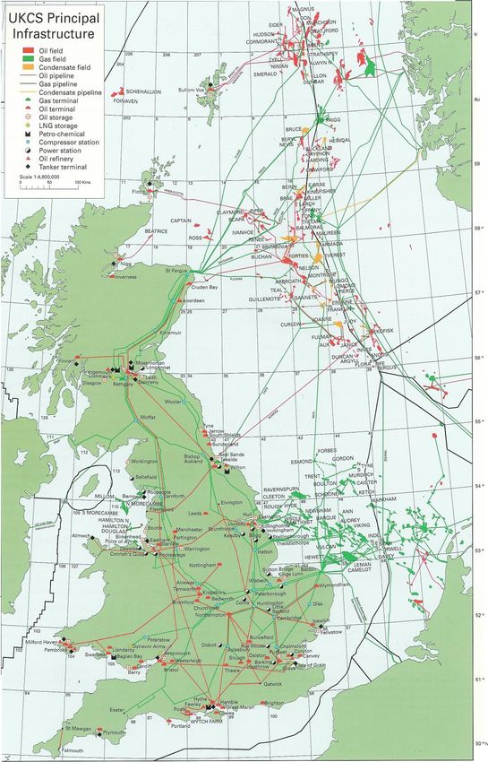
11(d) Characterisation of pipelines in the UKCS and elsewhere
Oil and gas in the UKCS are transported in an extensive pipeline network
and tankers. The total length of UK’s offshore oil and gas pipelines is
about 11,500 kilometres (BERR) of which roughly 5000 kilometres are in
the offshore-to-onshore direction. The offshore-onshore pipelines are of
direct interest to the present study because even though the CO2 would be
transported in the opposite direction, some of the pipelines and their
terminals could be re-used in CO2 transportation. In any case, they would
still be required to convey onshore any CO2-EOR oil that may be
produced in CCS projects.
To provide the context for a possible CO2 transportation network it is
useful to give a brief description of the length and diameters of the
offshore-onshore pipelines as presented in Tables 3 and 4. Table 3
presents descriptive statistics of the pipeline lengths.
12Table 3: Descriptive data on the lengths of the offshore-onshore pipelines in the
UKCS
Histogram of the lengths of the UKCS offshore-
onshore pipelines
Length (km)
12
Mean 140.57
Standard Error 24.38 10
Median 68.80
Mode 354
Standard Deviation 137.91 8
Sample Variance 19018.27 Frequency
Kurtosis 0.11
6
Skewness 1.17
Range 467.50
Minimum 5.60
4
Maximum 473.10
Sum 4498.10 2
Count 32
Largest(5) 354
0
Smallest(5) 29.60
50 100 150 200 250 300 350 400 450 500
Confidence Level
(95.0%) 49.72 kilometres
The descriptive statistics on the left panel in Table 3 show that there are
32 offshore-onshore pipelines ranging in length from a mere 6 kilometres
to about 480 kilometres, with the modal length being 354 kilometres and
the mean and median lengths being about 141 and 69 kilometres
respectively. The histogram in the right panel show that about 75 percent
of the pipelines are of lengths not exceeding 200 kilometres.
13Table 4 shows the descriptive statistics on the diameters of the pipelines.
Table 4: Descriptive data on the diameters of the offshore-onshore pipelines in
the UKCS
Histogram of the diameters of the UKCS
Diameter (mm)
offshore-onshore pipelines
12
Mean 683.81
Standard Error 30.27 10
Median 762.00
Mode 762.00
Standard Deviation 171.23
8
Sample Variance 29319.26
Kurtosis -0.04
Frequency
Skewness -0.80
6
Range 641.30
Minimum 273.10
Maximum 914.40
Sum 21882.00 4
Count 32
Largest(5) 863.60
Smallest(5) 508.00 2
Confidence Level (95.0%) 61.73
0
200 300 400 500 600 700 800 1000
diameters (mm)
Table 4 shows that the pipeline diameters range from 273 to 914 mm.
The modal diameter is 762mm while the mean and median diameters are
684 and 762 mm respectively. The histogram reveals that about 88
percent of the pipelines have diameters in excess of 600 mm.
In the United Kingdom, the CO2 transportation pipelines can consist of
both new build and re-used ones. Expected pipeline transportation costs
depend on a number of factors (see IPCC, 2005) including construction
costs, the age structure of the pipelines, the source-to-sink distance,
14geography (onshore/offshore lengths), pipeline diameters, and the
material conveyed (dry or wet CO2).
Given the relatively distant COP dates of many of the producing fields in
the CNS and NNS, most of the pipelines conveying CO2 to these sectors
will have to be new-build since most of the existing offshore-to-onshore
pipelines will still be transporting oil and gas and will not be available in
the medium term. The only pipeline in the CNS that is virtually ready for
re-use is the one linking the power plant at Peterhead to the Miller field
which is being decommissioned. However, greater pipeline re-use
opportunities exist in the SNS because of the imminence of the COP
dates of some of the gas fields.
Graph 1 gives an idea of how pipeline diameter and geography affect the
capital cost of pipeline networks according to the IEA.
Graph 1: Pipeline Diameters and Investment Costs (USA)
15Detailed construction costs of CO2 pipelines in the UK/UKCS are not
available because none has been constructed to date. The present study
assumed that a new-build CO2 pipeline transportation (of an average
0.762m or about 28-inch12 diameter) network in the UKCS would incur a
CAPEX of between £1 and £3 million per kilometre, with £2million/km
as the central value. This is higher than the IEA’s most recent estimate
for a pipeline of the same diameter at offshore USA presented in Graph 1,
and reflects the increased costs in recent years. The CAPEX of re-used
facilities is assumed to be lower than the stated amount. Specifically, it
was assumed that the existing pipelines in the SNS as well as the
Peterhead-Miller pipeline are modified and re-used at 50% of new-build
costs.
Graph 2 shows that economies of scale exist in CO2 transportation.
Graph 2:
Source: IPCC (2005)
12
That is, the median and modal diameter of the UKCS offshore-onshore pipelines (see Table 4 above).
16(e) Source-to-sink distances:
The distances between the i sources of CO2 and j EOR- and k Permanent
Storage- sinks are respectively denoted by diseor (i, j) and disperm (i, k)
in the model.
Using data on the locational co-ordinates (longitudes and latitudes) of
each sink and source, the shortest source-to-sink distances were
calculated using the Haversine formula13. The data on the source-to-sink
distances are in Table 5.
13
Haversine formula: d = R.c
where:
R = earth’s radius (mean radius = 6,371 km)
c = 2.atan2(a,(1-a))
a = sin2 (latitude/2) + cos (latitude1)cos (latitude2)sin2 (longitude/2)
latitude = latitude2 – latitude1
longitude = longitude2 – longitude1
1718
4. Scenario Analysis

The model was applied to investigate two important issues in CO2
transportation pertaining to (a) investment timing and (b) assumptions on
the minimum annual CO2 injectivity levels. CO2 can be transported into
permanent storage only when the gas and gas/condensate fields have been
depleted and made ready to receive it. By contrast, there is relative
flexibility in the CO2-EOR flooding start date, since the technology can
be deployed at anytime during secondary and/or tertiary oil production
(Bachu, 2004). This flexibility affects the availability of the fields to
receive CO2 and the consequent pipeline network configuration and costs.
A scenario analysis was conducted to investigate the most economical
way to distribute the captured CO2 under four scenarios, assuming two
alternative CO2-EOR injection commencement dates and two minimum
annual injectivity levels.

    (i) Scenario 1: Higher injectivity, with accelerated EOR start
        date

Scenario 1 is described as a higher injectivity and accelerated EOR start
date scenario. In the scenario the minimum CO2-EOR injectivity level of
5 MtCO2/year injectivity level is assumed. Furthermore, it is assumed
that CO2-EOR injection start dates for all the candidate fields is
accelerated to start uniformly during the 2018-2022 investment period.
Therefore, to qualify for inclusion in this scenario, a CO2-EOR sink must
have a minimum annual injectivity capacity of 5 MtCO2/year, if primary
CO2-EOR injection is carried out over a 15-year period.             CO2
transportation and injection into permanent storage, however, would be

                                                                      19
COP-led, with injection commencing immediately after a gas field is
depleted, and continuing throughout the study period.
(ii) Scenario 2: Lower injectivity with accelerated EOR start
dates
The assumptions of this scenario are the same as those in Scenario 1
except that the minimum annual injectivity is reduced to 3 MtCO2/year.
(iii) Scenario 3: Higher injectivity with COP-determined EOR
start dates
Scenario 3 uses the assumption that the CO2-EOR flooding starts 2 years
before the COP date of each selected field with the higher minimum
annual injectivity of 5 MtCO2/year. CO2 injection into permanent storage
starts immediately when a chosen gas field is depleted.
(iv) Scenario 4: Lower injectivity with COP date-determined
EOR start dates
Scenario 4 uses the same assumptions as Scenario 3 except for the
minimum injectivity which is reduced to 3 MtCO2/year.
5. Results:
Given the model, data parameters, and scenario assumptions, the model
solutions determined the quantities of CO2 transported into E0R and
permanent storage, indicating alternative pipeline network configurations.
The results are presented below.
20Scenario 1:
Scenario 1’s model solutions are presented below.
Table 6: Origination, destinations and volumes of CO2 transported and injected in Scenario 1
Pipelines only @ Distance
Sources Vt+1=Vt (km) type Terminal 2020 2025 2030 2035
Drax Forties 456 perm 8.33 10.66 14.81 20.47
Sub-total 8.33 10.66 14.81 20.47
Ferrybridge Ravenspurn 153 perm Easington 2.41 3.38 4.34 5.98
Sub-total 2.41 3.38 4.34 5.98
Killingholme West Sole 94 perm Easington 1.53 2.15 2.76 3.80
Sub-total 1.53 2.15 2.76 3.80
Kingsnorth Hewett 204 perm Bacton 3.02 4.23 5.44 7.49
Sub-total 3.02 4.23 5.44 7.49
Longannet Brae 436 3.70 5.18 6.47 8.99
Sub-total 3.70 5.18 6.47 8.99
Peterhead Claymore 139 EOR Peterhead 1.42 1.99 2.56 3.53
Sub-total 1.42 1.99 2.56 3.53
Teesside Morecambe South 227 perm Barrow-in-Furness 3.14 4.39 5.65 7.78
Sub-total 3.14 4.39 5.65 7.78
Tilbury Hewett 137 perm Bacton 1.46 2.05 2.63 3.63
Sub-total 1.46 2.05 2.63 3.63
Grand Total 25.01 34.03 44.66 61.67
The results of the system-wide optimisation of CO2 transportation costs
for Scenario 1 are shown in Table 6. They shed light on some of the
21issues concerned with CO2 transportation and sequestration in the
UK/UKCS.
CO2 shipments over relatively long distances such as those from Drax to
Forties (conveying between 8 and 20 MtCO2/year) are possible because
several studies (see ISGS (2005), IPCC (2005) and Middleton and
Bielicki (2009), for examples) have emphasised the economies of scale
present in CO2 transportation. With the possibility of reaping the fruits of
scale economies nearness to a source can be less important than the mass
flow rate or the volume of CO2 transported to a sink. Of course,
economies of scale do exist over short distances as well, which is why it
seems paradoxical that the model solution allocates Drax’s output to
Forties instead of to Morecambe South, a large permanent storage sink
only about 168 kilometres away from Drax. However, an inspection of
the detailed results revealed that, while Drax can ship CO2 to Morecambe
South for most of the study period without increasing the optimised
system transportation cost, doing so in 2030 violates this condition.
Specifically, Drax-Morecambe South shipments in 2030 are sub-optimal
and inadmissible because they increase overall network system costs by
about £9.8 million. In a setting or model that permits it, the Drax-
Morecambe South deliveries would have been temporary. However, the
constraints (equations 8 and 9) of the present model prohibit temporary
CO2 deliveries.
In order to test the extent of the scale economies in the model solution
both the optimised total and average capital costs functions were
specified and estimated. The implied economies of scale were estimated
using a double-log regression equation of the total capital cost on the total
CO2 shipments and yielded the following result:
22ln(total CAPEX) = 2.273 + 0.886ln(cumulative CO2 shipment volumes)
(3.036) (5.005) adjustedR2 = 0.77
where:
ln = natural logarithm
t-statistics are in brackets
Using the slope of the regression, the estimated economies of scale factor
is 1.129, indicating the presence of substantial scale economies implicit in
the optimised pipeline capital costs. A graphical illustration of the
average capital cost function is presented in Graph 3.
Graph 3: UKCS: CO2 pipeline transportation average capital cost curve: Scenario 1
14
12
Cost (£/tCO2/100 km)
10
8
6
4
2
0
1 2 3 4 5 6 7 8
MtCO2/year transported and injected
The concavity of the average capital cost curve indicates the presence of
both the economies of scale and full pipeline utilisation. Exploiting the
benefits of scale economies, close matching of source-sink capacities14,
and minimisation of system-wide costs throughout the study period, are
the reasons why Drax can ship CO2 to Forties instead of to nearer sinks,
14
For example, wwithout CO2 deliveries from the largest CO2 capture plant (Drax), Forties’
injectable maximum 20 MtCO2/year would have been met from smaller capture plants at higher costs
to the overall system.
23such as Morecambe South. CO2 deliveries are made to Morecambe South
from Teesside (181 km) in this scenario.
One effect of promoting only the large CO2-EOR projects capable of
handling a minimum annual injectivity of 5 MtCO2/year over 15 years in
this scenario, is to exclude sinks with smaller injectivity. Notably, Miller
was dropped from the analysis in this scenario, leaving Beryl, Brae,
Claymore, Forties, Nelson and Ninian in contention for CO2 allocations
from the sources. In the event, the model solution allocated the captured
CO2 among (a) three oilfields – Forties, Brae and Claymore – from the
three power stations at Drax, Longannet and Peterhead, and (b) four
permanent storage sinks – Ravenspurn, West Sole, Morecambe South and
Hewett – from the remaining five power plants in the study.
It is noteworthy, however, that in a few cases the optimised CO2
deliveries and injection levels diverge from the minimum injectivity
level. The divergence is inevitable given that the CO2 supply capacities
are built-up over time (for example, Ferrybridge and its shipments to
Ravenspurn) and the maximum capture capacities of some plants are less
than 5 MtCO2/year in any case.
Also, it is noteworthy that cumulative shipments of CO2 in excess of 100
MtCO2 would be delivered to two sinks –one CO2-EOR (Forties) and the
other permanent storage (Hewett) over the time period to 2037.
Specifically, the Forties field would receive very close to 200 MtCO 2
while Hewett would receive roughly 115 MtCO2 from the power plants at
Kingsnorth and Tilbury. Brae is the third largest repository of CO2 in this
scenario.
24The annual CO2 mass flow rate rates range between 3 MtCO2/year to
about 14 MtCO2/year. In all, the total length of the pipelines to be
constructed in this scenario is about 1850 kilometres. Based on the
Kinder Morgan (2009) experience, a crude approximation of the implied
pipeline diameters is set out in Table 7
Table 7: Scenario 1: Conceptual pipeline routes and pipeline
diameters
estimated estimated
diameters diameters
Source Sink (mm) (inches)
Drax Forties 914.84 36.02
Ferrybridge Ravenspurn 451.84 17.79
Killingholme West Sole 384.09 15.12
Kingsnorth Hewett 497.31 19.58
Longannet Brae 516.58 20.34
Peterhead Claymore 368.23 14.50
Teesside Morecambe South 504.16 19.85
Tilbury Hewett 372.01 14.65
Table 7 indicates that the pipeline diameters range from roughly 368 (or
15”) to 915 mm (or 36”). These are well within the range of pipelines
currently in use in the UKCS.
The total CAPEX required in this scenario is about £4bn for pipeline
lengths varying from 94 km to 456 km, and diameters varying from 368
to 915 mm. The average capital cost varies from £1 to about
£5/tonne/100 km.
25Having identified the pipeline routes in this scenario a conceptual
pipeline network configuration based on the model solutions is presented
in Map 215.
15
The authors’ conceptual pipeline routes (in arrows) in Maps 2 to 5 are superimposed on an original
map compiled by BERR.
26Map 2: Conceptual CO2 Pipeline routes in Scenario 1
Peterhead
Longannet
Teesside
Ferrybridge
Drax
Killingholme
Tilbury
Kingsnorth
27Scenario 2: Accelerated CO2-EOR start date (3 MtCO2/year minimum injectivity)
Table 8: Origination, destinations and volumes of CO2 transported and injected in Scenario 2
Sources Pipelines only @ Distance type Terminal 2020 2025 2030 2035
Vt+1=Vt (km)
Drax Forties 456 perm 8.33 10.66 15.00 16.09
Drax Ravenspurn 140 perm Easington 3.22
Drax West Sole 146 perm Easington 1.35
Sub-total 8.33 10.66 15.00 20.66
Ferrybridge Ravenspurn 153 perm Easington 2.41 3.38 4.34 5.98
Sub-total 2.41 3.38 4.34 5.98
Killingholme West Sole 94 perm Easington 1.53 2.15 2.76 3.80
Sub-total 1.53 2.15 2.76 3.80
Kingsnorth Hewett 204 perm Bacton 3.02 4.23 5.44 7.49
Sub-total 3.02 4.23 5.44 7.49
Longannet Brae (East) 436 3.70 3.70 3.95 6.47
Longannet Forties 341 perm 1.48 2.71 2.71
Sub-total 3.70 5.18 6.66 9.18
Peterhead Miller 234 eor Peterhead 1.42 1.99 2.56 3.53
Sub-total 1.42 1.99 2.56 3.53
Teesside Morecambe South 227 perm Barrow-in-Furness 3.14 4.39 5.65 7.78
Sub-total 3.14 4.39 5.65 7.78
Tilbury Hewett 137 perm Bacton 1.46 2.05 2.63 3.63
Sub-total 1.46 2.05 2.63 3.63
Grand Total 25.01 34.03 45.04 62.05
The results for Scenario 2 are shown in Table 8. There are a few
instances of one source shipping CO2 to more than one sink in this
scenario. Source-to-multiple sinks deliveries occur in the model because
once the annual CO2 deliveries to and injection into a sink equal the
sink’s injectivity level for that year, any excess CO2 available at the
28supplying source is shipped to another sink. Thus, for example, while the
injectivity levels at Brae are 3.70 MtCO2/year (2018-2022), 3.70 (2023-
2027), 3.95 (2028-2032) and 6.47 MtCO2/year (2033-2037) the CO2
supply capacities at Longannet during the corresponding period are 3.70,
5.18 , 6.66 and 9.18 MtCO2/year. Clearly, apart from the initial period,
Longannet has an excess capacity to satisfy the injectivity levels at Brae,
which it disposes of by finding another outlet.
The cumulative total volume of CO2 shipped from the sources to the
various sinks in this scenario is about 831 MtCO2 over the period to 2037,
yielding an annual average shipment of about 42 MtCO2/year.
Unsurprisingly, this is about the same as in Scenario 1 (41 MtCO2/yr).
Interestingly, the same number of CO2-EOR- and permanent storage
sinks are determined to be optimally reachable in this scenario as in
Scenario 1. Moreover, the same four permanent storage sinks –
Ravenspurn, West Sole, Hewett and Morecambe South – were found to
be accessible in this scenario as well. Regarding the CO2-EOR sinks,
however, the Miller field replaced Claymore as the third CO2-EOR sink.
Having qualified for inclusion in this scenario because it met the 3
MtCO2/year injectivity level criterion, Miller displaced Claymore as the
destination of the CO2 captured at Peterhead. CO2 is shipped from
Peterhead to Miller in spite of the longer distance (234 versus 139
kilometres) because it is cheaper to re-use the existing Peterhead-Miller
pipeline than build a new Peterhead-Claymore pipeline.
Forties remains the largest destination of CO2, receiving a cumulative
total of almost 300 MtCO2 from two sources – Drax and Longannet –
instead of the one source (Drax) in Scenario 1. The difference in the CO2
transportation patterns is caused by the difference in the phasing of the
29injection through time. In Scenario 1 the CO2-EOR injection period was
reduced to 15 years, raising the minimum injectivity level, (hence pipe
sizes) while the primary CO2-EOR injection period in Scenario 2 is
increased to 20 years thereby lowering the minimum injectivity level (and
pipe sizes) Thus, for example the maximum injectivity level at Brae in
Scenario 1 is about 8-9 MtCO2/year, virtually matching Longannet’s
supply capacity which, having no excess supply has no need for another
sink. However, by elongating the injection period in Scenario 2 to 20
years, the maximum injectivity is reduced to about 5-6 MtCO2/year,
leaving Longannet with a potential ultimate excess supply capacity of
about 3 MtCO2/year, hence the recourse to a second sink.
Ravenspurn and West Sole also receive CO2 from two sources each
instead of the single sources in Scenario 1. Both sinks receive the supply
“overflows” from Drax in addition to their respective supplies from
Ferrybridge and Killingholme. Hewett remains the second largest
destination, but Brae is relegated to the fifth position, having been
overtaken by Morecambe South and Ravenspurn. Less CO2 was shipped
to Brae from Longannet in this scenario because the injectivity level was
lowered.
In general, the annual mass flow rate in this scenario is lower than in
Scenario 1, implying smaller pipeline diameters. However, the total
volume of CO2 transported and injected is about 34 percent higher than in
Scenario 1. Two closely-related factors account for this. The first is the
investment timing advantage of Scenario 2. Spreading the CO2
(especially CO2-EOR) and transportation and injection investment over a
longer time period, especially the last five years of the study period when
full supply capacity is attained, implies that Scenario 2 better
30synchronises the required CO2 injectivity levels with the pace of the
supply capacity expansion. By contrast, Scenario 1 suffers a relative
investment timing disadvantage because the accelerated CO2-EOR
projects are “front-loaded”, requiring higher CO2 injectivity levels (5
MtCO2/year) to be met in the first 15 years from 2018, when the system’s
CO2 supply capacity has been developed. Thus, there is a greater
mismatch of the respective storage and production capacities of the sinks
and sources, or between injectivity and injection levels in this scenario.
How well the two scenarios are able to meet the injectivity requirements
are shown in columns 6 and 7 of Table 9 below.
Table 9: A comparison of injectivity-injection ratios in Scenarios 1 and 2
Cumulative CO2
shipment (MtCO2) injection as % of
Eventual
injectivity
storage
Sinks Sources
capacity
(MtCO2)
Scenario Scenario Scenario Scenario
1 2 1 2
1 2 3 4 5 6 7
Brae Longannet 117 93.66 89.1 80.05 76.15
Claymore Peterhead 60 36.58 60.97 0.00
Forties Drax 282 193.94 247.5
Longannet 34.5
sub-total
(Forties) 282 193.94 282 68.77 100.00
Hewett Kingsnorth 381 77.7 100.9
Hewett Tilbury 37.62 48.85
sub-total
(Hewett) 381 115.32 149.75 30.27 39.30
Miller Peterhead 53 47.5 0.00 89.62
Morecambe
South Teesside 529 80.7 104.8 15.26 19.81
Ravenspurn Ferrybridge 138 62.03 80.55
Drax 16.1
sub-total
(Ravenspurn) 138 62.03 96.65 44.95 70.04
West Sole Killingholme 125 39.43 51.2
Drax 6.75
sub-total 125 39.43 57.95 31.54 46.36
Grand total 1685 621.66 827.75 36.89 49.12
31Clearly, the lower annual injectivity requirement of Scenario 2 is better
matched with the build-up of the supply capacities, especially taking full
advantage of the build-up to 100 percent capacity in the last investment
cycle to increase CO2 shipments .along the same routes identified in
Scenario 1. Such increases account for two-thirds of the overall increase.
The evolution of additional pipeline routes in Scenario 2 accounted for
the remaining one-third difference. The additional pipeline routes are the
Longannet-Forties, Peterhead-Miller, Drax-Ravenspurn, and Drax-West
Sole. The higher level of CO2 shipments in Scenario 2 necessitated more
pipeline resources, hence the overall length of pipelines in this scenario
exceeds that in Scenario 1 by about 40 percent.
Table 10: Scenario 2: Conceptual pipeline routes and pipeline diameters
estimated estimated
diameters diameters
Source Sink (mm) (inches)
Drax Forties 761.80 29.99
Drax Ravenspurn 357.26 14.07
Drax West Sole 291.06 11.46
Ferrybridge Ravenspurn 451.84 17.79
Killingholme West Sole 384.09 15.12
Kingsnorth Hewett 497.31 19.58
Longannet Brae 428.53 16.87
Longannet Forties 310.72 12.23
Peterhead Miller 354.66 13.96
Teesside Morecambe South 504.16 19.85
Tilbury Hewett 372.01 14.65
The total pipeline CAPEX is about £5 bn for pipeline lengths varying
from 94 km to 456 km. This is about £1 bn costlier than Scenario 1, but
more CO2 is transported and injected in Scenario 2. The average capital
cost varies from £0.8/tonne/100 km to about £6/tonne/100 kilometres in 9
out of the 11 pipeline routes. The average costs of the two remaining
32pipeline routes from Drax to Ravenspurn and West Sole are outliers at
£12 and £28/tonne/100 km respectively, raising the question of why the
shipments have been selected by the model. From the results it is seen
that the deliveries to Ravenspurn and West Sole are overflows or the
excess of supply capacity (at Drax) over the CO2 injection requirements
at Forties (18.80 MtCO2/year) which Drax was supplying up to the last
investment period (2033 -2037). The excess supply has to be disposed
off in other sinks, at minimum increase in the overall transport cost16.
Specifically, since one of the model assumptions is the re-use of the SNS
pipelines (Ravenspurn-Easington and West Sole-Easington), it is
plausible that the two deliveries would be combined and delivered into
one Drax-Easington pipeline. At Easington, the CO2 would be routed
appropriately.
In estimating the total capital transport cost function, it was found that a
linear cost function fitted the data better than the double-log function.
The estimated linear total cost function is17:
(total CAPEX) = 284.8488 + 2.411(cumulative CO2 shipment volumes)
(3.036) (2.535) adjusted R2 = 0.35
Thus, in spite of the apparent anomalies, the estimated scale economies at
about 1.565 are more substantial in this scenario than in Scenario 1. The
optimised average CO2 transportation capital cost curve of this scenario is
presented in Graph 4.
16
The other ways and manners of disposal of the excess CO2 are beyond the scope of the present study.
17
For the interested reader, the estimated log-linear total cost function is:
ln (total CAPEX) = 4.969 + 0.266ln (cumulative CO 2 shipment volumes)
(8.171) (1.783) adjusted R 2 = 0.19
33Graph 4: UKCS: CO2 pipeline transportation average cost curve: Scenario 2
12
10
Cost (£/tCO2/100 km)
8
6
4
2
0
1 2 3 4 5 6 7 8
MtCO2/year transported and injected
A conceptual CO2 pipeline transportation network based on Scenario 2’s model
solutions is presented below in Map 3.
34Map 3: Conceptual CO2 Pipeline routes in Scenario 2
Peterhead
Longannet
Teesside
Ferrybridge
Drax
Killingholme
Tilbury
Kingsnorth
35Scenario 3: COP-driven EOR start date with offset (i.e. EOR-oil revenue credits)
Table 11: Origination, destinations and volumes of CO2 transported and injected in Scenario 3
Sources Pipelines only @ Distance type Terminal 2020 2025 2030 2035
Vt+1=Vt (km)
Drax Forties 456 eor 2.33 6.67 12.33
Ravenspurn 140 perm 3.80 3.80 3.80 3.80
West Sole 146 perm 4.53 4.53 4.53 4.53
Sub-total 8.33 10.66 15.00 20.66
Ferrybridge Ravenspurn 153 perm Easington 2.41 3.38 4.34 5.98
Sub-total 2.41 3.38 4.34 5.98
Killingholme West Sole 94 perm Easington 1.53 2.15 2.76 3.80
Sub-total 1.53 2.15 2.76 3.80
Kingsnorth Hewett 204 perm Bacton 3.02 4.23 5.44 7.49
Sub-total 3.02 4.23 5.44 7.49
Longannet Brae 436 eor/perm 3.70 3.70 5.05 7.57
Forties 341 eor 1.48 1.61 1.61
Sub-total 3.70 5.18 6.66 9.18
Peterhead Brae 228 eor/perm 1.42 1.42 1.42 1.42
Claymore 139 eor Peterhead 0.57 1.14 2.10
Sub-total 1.42 1.99 2.56 3.52
Teesside Morecambe South 227 perm Barrow-in-Furness 3.14 4.39 5.65 7.78
Sub-total 3.14 4.39 5.65 7.78
Tilbury Hewett 137 perm Bacton 1.46 2.05 2.63 3.63
Sub-total 1.46 2.05 2.63 3.63
Grand Total 25.01 34.03 45.04 62.04
The results for Scenario 3 are shown in Table 11. Scenario 3 is different
because unlike the earlier scenarios, the transportation and injection of
CO2-EOR are driven by the COP dates of the fields, rather than via any
deliberate effort to accelerate CO2-EOR start dates. Scenario 3 shares
36some of the assumptions of Scenario I, particularly the assumption of a 5
MtCO2/year reservoir minimum injectivity.
The model solutions of this scenario are a hybrid of the earlier scenarios.
Thus the three favoured CO2-EOR sinks are the Forties, Brae and
Claymore fields while the permanent storage sinks and the respective
CO2 sources remain the same as well. Furthermore, the cumulative total
volumes of CO2 transported and injected at approximately 612 MtCO2 are
about the same as in Scenario 1.
In common with Scenario 2, the model solutions of Scenario 3 yielded a
relatively lengthy pipeline infrastructure of about 2701 km. Lengthier
pipelines are the direct consequence of introducing timelines into the
scenario. In matching sources and sinks, timeline considerations force the
least-cost transportation model to recognise that some sinks, even though
nearer (that is, located at least-cost distances to some sources), may not
be ready to receive CO2 as and when it is available at the sources. Thus,
a distant but available sink would be served at first, but, when all the
sinks become available and they compete for CO2 allocation on an equal
footing, the least cost algorithm would allocate deliveries to the nearby
cheaper sinks as well.
37Table 12: Scenario 3: Conceptual pipeline routes and pipeline diameters
estimated estimated
diameters diameters
Source Sink (mm) (inches)
Drax Forties 630.42 24.82
Drax Ravenspurn 377.52 14.86
Drax West Sole 402.17 15.83
Ferrybridge Ravenspurn 451.84 17.79
Killingholme West Sole 384.09 15.12
Kingsnorth Hewett 497.31 19.58
Longannet Brae 466.96 18.38
Longannet Forties 272.29 10.72
Peterhead Brae 281.79 11.09
Peterhead Claymore 318.27 12.53
Teesside Morecambe South 504.16 19.85
Tilbury Hewett 372.01 14.65
Scenario 3’s total CAPEX is roughly £5.4 billion, being larger than in the
earlier scenarios. The estimated cost function was:
ln (total CAPEX) = 13.765 - 4.827ln (cum CO2 shipment) + 0.711ln (cum CO2 shipment)2
(2.733) (-1.592) (1.62) adjusted R2 = 0.06
The economies of scale were found to be variable18, requiring a higher
threshold of CO2 shipments before scale economies kick-in. The
estimated economies of scale on the quadratic term in log cumulative
shipments is 1.40. The annual mass flow rate ranges between 1.42 and
8.42 MtCO2/year while average capital cost varies between £2.48 and
£9.39/tonne/100 km in ten out of the twelve pipeline routes. The outliers
with £15.85 and £16.92/tonne/100 km respectively are the Longannet-
Forties and Peterhead-Claymore pipeline routes. The outlier costs are
generated by the timeline effects described above. Both Peterhead and
Longannet had to ship CO2 to the relatively distant sink (Brae) initially
18
That is, the estimated regression model with variable scale economies was better behaved than the
fixed scale model.
38because the nearer sinks (Forties, in the case of Longannet and Claymore,
in the case of Peterhead) were not available.
The average capital cost function is presented graphically below in Graph
5.
Graph 5: UKCS: CO2 pipeline transportation average cost curve: Scenario 3
20
16
Cost (£/tCO2/100 km
12
8
4
0
1 2 3 4 5 6 7 8
MtCO2/year transported and injected
A conceptual CO2 pipeline transportation network based on Scenario 3’s
model solutions is presented below in Map 4.
39Map 4: Conceptual CO2 Pipeline routes in Scenario 3
Peterhead
Longannet
Teesside
Ferrybridge
Drax
Killingholme
Tilbury
Kingsnorth
40Scenario 4: COP-driven EOR start date with no offset (i.e. EOR-oil revenue credits excluded)
Table 13: Origination, destinations and volumes of CO2 transported and injected in Scenario 4
Sources Pipelines only @ Distance (km) type Terminal 2020 2025 2030 2035
Vt+1=Vt
Drax Morecambe South 168 perm Barrow-in-Furness 6.93 6.93 6.93 6.93
Drax Ravenspurn 140 perm Easington 1.40 3.73 8.07 9.20
Drax West Sole 146 perm Easington 4.53
Sub-total 8.33 10.66 15.00 20.66
Ferrybridge Morecambe South 159 perm Barrow-in-Furness 2.41 3.38 4.34 5.98
Sub-total 2.41 3.38 4.34 5.98
Killingholme West Sole 94 perm Easington 1.53 2.15 2.76 3.80
Sub-total 1.53 2.15 2.76 3.80
Kingsnorth Hewett 204 perm Bacton 3.02 4.23 5.44 7.49
Sub-total 3.02 4.23 5.44 7.49
Longannet Morecambe South 246 perm Barrow-in-Furness 3.70 5.18 6.66 9.18
Sub-total 3.70 5.18 6.66 9.18
Peterhead Miller 234 eor Peterhead 1.42 1.99 2.56 3.53
Sub-total 1.42 1.99 2.56 3.53
Teesside Morecambe South 227 perm Barrow-in-Furness 3.14 4.39 5.65 7.78
Sub-total 3.14 4.39 5.65 7.78
Tilbury Hewett 137 perm Bacton 1.46 2.05 2.63 3.63
Sub-total 1.46 2.05 2.63 3.63
Grand Total 25.01 34.03 45.04 62.05
The results of Scenario 4 are shown in Table 13. A feature of the model
solution in Scenario 4 is that only the Peterhead-Miller route emerged as
a viable candidate for CO2-EOR shipments. Clearly, re-using the existing
Peterhead-Miller pipeline boosted the chances of this particular route.
41Having to build new pipelines without the cushion effects of the CO2-
EOR oil revenues on CO2 transport costs, but with relative delays in the
injection start-up dates, the remaining CO2-EOR sinks were at a relative
transport cost disadvantage vis-à-vis the permanent storage fields in the
SNS to which the model solution routed the bulk of the CO2.
The cumulative total volume of CO2 transported and injected in this
scenario is 831 MtCO2 in the period to 2037, the same as in Scenario 2.
Of this, the bulk – about 448 MtCO2 (or 54 percent) – is transported from
four sources – Drax, Ferrybridge, Longannet and Teesside – and injected
into permanent storage in Morecambe South. In this scenario CO 2 could
be transported from Ferrybridge and Drax to Morecambe South in a
communal pipeline.
In general, the variability in the annual average mass flow rates in this
scenario is relatively lower, ranging between 2.27 and 6.93 MtCO2/year,
requiring pipe sizes in the range of 14 to 22 inches.
Table 14: Scenario 4: Conceptual pipeline routes and pipeline diameters
estimated estimated
diameters diameters
Source Sink (mm) (inches)
Drax Morecambe South 482.89 19.01
Drax Ravenspurn 566.20 22.29
Drax West Sole 402.17 15.83
Ferrybridge Morecambe South 450.98 17.76
Killingholme West Sole 384.09 15.12
Kingsnorth Hewett 497.31 19.58
Longannet Morecambe South 550.36 21.67
Peterhead Miller 354.66 13.96
Teesside Morecambe South 504.16 19.85
Tilbury Hewett 372.01 14.65
42You can also read