Forecasting Future Murders of Mr. Boddy by Numerical Weather Prediction
←
→
Page content transcription
If your browser does not render page correctly, please read the page content below

Forecasting Future Murders of Mr. Boddy by Numerical Weather Prediction
                                                                                                         Eve Armstrong∗1,2
                                                                 1 Computational   Neuroscience Initiative, University of Pennsylvania, Philadelphia, PA 19104, USA
                                                                         2 Departmentof Physics, New York Institute of Technology, New York, NY 10023, USA

                                                                                                     (Dated: April 1, 2019)
arXiv:1903.12604v1 [physics.pop-ph] 29 Mar 2019

                                                                                                             Abstract

                                                     Despite a previous description of his state as a stable fixed point, just past midnight this morning Mr. Boddy
                                                     was murdered again. In fact, over 70 years Mr. Boddy has been reported murdered 106 times, while there exist
                                                     no documented attempts at intervention. Using variational data assimilation, we train a model of Mr. Boddy’s
                                                     dynamics on the time series of observed murders, to forecast future murders. The parameters to be estimated
                                                     include instrument, location, and murderer. We find that a successful estimation requires three additional elements.
                                                     First, to minimize the effects of selection bias, generous ranges are placed on parameter searches, permitting
                                                     values such as the Cliff, the Poisoned Apple, and the Wife. Second, motive, which was not considered relevant to
                                                     previous murders, is added as a parameter. Third, Mr. Boddy’s little-known asthmatic condition is considered as
                                                     an alternative cause of death.
                                                         Following this morning’s event, the next local murder is forecast for 17:19:03 EDT this afternoon, with a
                                                     standard deviation of seven hours, at The Kitchen at 4330 Katonah Avenue, Bronx, NY, 10470, with either the
                                                     Lead Pipe or the Lead Bust of Washington Irving. The motive is: Case of Mistaken Identity, and there was no
                                                     convergence upon a murderer. Testing of the procedure’s predictive power will involve catching the D train to
                                                     205th Street and a few transfers over to Katonah Avenue, and sitting around waiting with our eyes peeled. We
                                                     discuss the problem of identifying a global solution - that is, the best reason for murder on a landscape riddled
                                                     with pretty-decent reasons. We also discuss the procedure’s assumption of Gaussian-distributed errors, which will
                                                     under-predict rare events. This under-representation of highly improbable events may be offset by the fact that the
                                                     training data, after all, consists of multiple murders of a single person.

                                                                                                    I.    INTRODUCTION

                             When we last visited Mr. Boddy Sylvester van Meers-                                      poses, with the aim of intervention or even just for sport.
                         bergen, he lay motionless on the concrete floor of an                                        Yet a method of prediction is readily at hand. In the
                         aviary in Philadelphia, Pennsylvania, just west of the                                       field of numerical weather prediction, it is called data
                         Schuylkill River [1]. His dynamics had transitioned from                                     assimilation.
                         a limit cycle, via an Andronov-Hopf bifurcation that has                                         Data assimilation (DA) was invented to predict the
                         since been attributed to Colonel Mustard with the Can-                                       weather [6, 7, 8, 9]. It is a means to exploit information
                         dlestick. The medical authorities present at the time                                        in observable data to complete a dynamical model of the
                         concurred that his configuration represented an asymp-                                       physical system that generated the data. This model may
                         totically stable equilibrium. Nevertheless, within mere                                      have unknown parameters to be estimated, and may in-
                         minutes Mr. Boddy was murdered again [2].                                                    clude state variables that are not observed. If the transfer
                             In fact, in the interim year Mr. Boddy has been re-                                      of information from measured to unmeasured quanti-
                         ported murdered 14,322 times [3], most recently just this                                    ties is efficient, the completed model can be integrated
                         morning [4]. Moreover, there exists a 70-year time se-                                       forward to predict future data. DA differs from the for-
                         ries of such reports [5], with a mean frequency of 10−3                                      mulation of machine learning in that it assumes that the
                         Hz. To our knowledge, no attempt has been made at                                            data were generated by a physical system rather than
                         employing this record of observations for predictive pur-                                    sorcery [10].
                                                  ∗ aeve@sas.upenn.edu

                                                                                                                  1
The DA framework is apt for capturing the case of                   reported deaths. Specifically, we place generous limits
Mr. Boddy. Mr. Boddy is a known dynamical system,                       on the search ranges of all parameter values, tossing in
who at any time is observable as either Alive or Dead1 .                extremely-likely (Figure 1) and extremely-unlikely (Fig-
His trajectory in state space can be described in terms                 ure 2) values that have never been reported. For example,
of Markov transition probabilities, which, importantly,                 Undercooked Chicken (likely) and the Poisoned Apple
capture his ability to instantly forget having died.                    (unlikely) are included as instruments. We also allow
    Multiple external parameters act upon Mr. Boddy,                    each candidate murderer to disguise him-or-herself as
including instrument, location, and murderer, and at any                any other candidate murderer, so that a serial killer may
timepoint on his trajectory each parameter takes a spe-                 be pulling off the entire time series single-handedly2 .
cific value. We would like to use the record of reported                    Third, we consider Mr. Boddy’s little-known severe
deaths to estimate those parameters at each instance on                 asthmic condition: occasionally, Mr. Boddy becomes fa-
the trajectory, to predict future instances of death. The               tally allergic to breathing. His general practitioner attests
70-year time series of observations is significantly longer             that it is as likely a cause of death as is murder [11], even
than the temporal distance between murders. Thus we                     given the observed murder frequency. Thus, we add as
have a decent shot at using that record to predict a small              an unobserved state variable Mr. Boddy’s level of Im-
distance into the future.                                               munoglobulin E (IgE) antibodies. Heightened levels of
    We find that several additional ingredients are re-                 IgE antibodies indicate an overreaction to allergens, and
quired to converge on a solution. First we need motive,                 are associated with fatality in some autopsies [12].
or more generally, “reason”, as a fourth parameter gov-                     The DA procedure used in this paper is an optimiza-
erning Mr. Boddy’s dynamics. Second, we ameliorate the                  tion wherein a cost function is minimized. We discuss
selection bias introduced by using information only from                details of the procedure, including the problem of iden-

Figure 1: Highly likely values of θmurder that may have been historically undersampled. (Left-to-right, top-to-bottom:
[13, 14, 15, 16, 17, 18, 19, 20, 21].)

  1 Quantum      considerations are beyond the scope of this paper; see Discussion.
  2 “Serial   killer” refers to multiple murders by one person. We permit a special case of multiple murders by one person of one person.

                                                                                                                                            2
Figure 2: Highly unlikely values of θmurder , tossed into the parameter search ranges for good measure. *Too nice. **Too
obvious. (Left-to-right, top-to-bottom: [22, 23, 24, 25, 26, 27, 28, 29, 30].)

tifying a minimum that is low enough to satisfy our pre-                   The first murder forecast within the local region is
dictive purposes. Our predictive purposes are not yet                  late this afternoon. We are reasonably confident that this
clear to us, and so at the moment this is not a high-                  will happen, as a preliminary DA prediction that used an
priority concern. The procedure also assumes Gaussian                  80-versus-20% (trial-versus-test) split of the 70-year time
errors, which will under-predict rare events. This is                  series reached one Lyapunov time in one week. That is,
troublesome, as rare events - when they do occur - are                 we won’t reach the limit of predictability until April 8.
typically the most unsettling. And, at least in the case of            Well, only time will tell. Now we wait.
the weather, the most deadly.

                                                            II.   MODEL

    In this Section we define Mr. Boddy’s dynamical map.               ward mapping for the physical system under study, the
Let a model f : Xn → Xn+1 define a forward mapping                     parameters are external forces whose underlying dynam-
of a dynamical system X. We assume Markov chain                        ics are unknown.
transition probabilities [31], where the state of the sys-                 For the purposes of this study, the only important
tem at time (n + 1) is entirely determined by the state at             characteristic of Mr. Boddy is whether he is alive or
time n. This is an important feature for Mr. Boddy, who                dead. This is a directly observable quantity with a 70-
evidently forgets having been murdered just a timestep                 year record of reported values (Figure 3), and we define
ago. The model is a function of dynamical variables x                  it as a state variable. Now, in initial tests of the DA pro-
and of any unknown model parameters θ, where the                       cedure, when we wrote Mr. Boddy’s state solely in terms
parameters themselves may be time-varying. That is,                    of this one state variable, there was no convergence on
X ≡ [xt=0 , xt=1 , ..., xt=T , θt=0 , θt=1 , ..., θt=T ], where T is   a solution. For this reason, we consulted Mr. Boddy’s
the final time step. The parameters are distinguished                  general practitioner to ask whether we were missing a
from the state variables because, while we write a for-                piece of the picture. It turns out that in addition to his

                                                                                                                                 3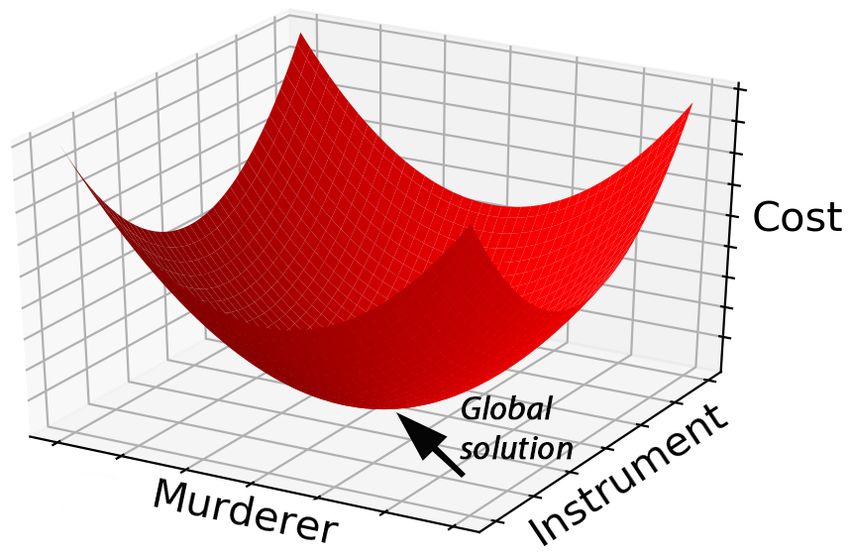
Figure 3: Time series of observations, modeled as Markov-chain transitions from Alive to Dead. Top: Full 70-year time
series. The jumps cannot be resolved by-eye. Bottom: Zoom-in on the final 23 hours. Alive-to-dead transitions are governed by
the transition probabilities of Equation Set 2; dead-to-dead transitions do not occur.

proclivity to being murdered, there exists another likely              examine the coupling of x and y. If the value of y at time
means for Mr. Boddy to transition to Dead: a severe                    n (denoted yn ) is above ythresh , then xn+1 , by definition of
asthmatic condition (see Introduction for references). We              ythresh , will be −1; that is, Mr. Boddy will die from an
thus added an unmeasured state variable: Mr. Boddy’s                   asthma attack. On the flip side, if xn = −1 already, then
level of IgE antibodies3 .                                             y will not evolve in the interim before time (n + 1), as Mr.
    The dynamical system is defined, then, in terms of                 Boddy’s biological processes have momentarily ceased to
two state variables: x ≡ [ x, y], where x is the Alive-                run. Neither of these cases is particularly interesting.
versus-Dead state and y is the level of IgE antibodies.                    A more tantalizing scenario presents itself when
The parameters governing murder (θmurder ≡ [instrument,                xn = 1 and yn < ythresh . At such a time, Mr. Boddy
location, murderer, reason]) are distinct from those gov-              is alive and will not die from asthma within the next time
erning asthmatic condition (θasthma ≡ [concentration of                step - and thus we can focus on murder probability. Let’s
airborne Alternaria4 , and other environmental factors5 ]). Note       examine this simplified (i.e. no-asthma-attack) regime,
also the addition of reason as a parameter, which is re-               focusing on variable x, and recouching the equations in
quired for solutions to converge. Some reasons are listed              terms of probabilities. We write:
in Table 1.
    We now write the continuous-time dynamics most                        P( xn+1 = −1| xn = 1, yn < ythresh ) = f x (θmurdern );
                                                                                                                                        (2)
generally as:                                                             P( xn+1 = −1| xn = −1, yn < ythresh ) = 0.
            dx                                                         The first line in Equation Set 2 states that the probability
               = f x ( x (t), y(t, ythresh ), θmurder (t));
            dt                                                   (1)   of transitioning from Alive to Dead, given yn < ythresh , is
            dy                                                         some function of the parameters θmurder . The second line
               = f y ( x (t), y(t, ythresh ), θasthma (t)),
            dt                                                         states that the probability of transitioning from Dead to
where the affine parameterization t is time, y is continu-             Dead is zero (a step function will be employed to transi-
ous, and x may take discrete binary values of 1 (Alive)                tion him back to Alive). In other words, the probability
or −1 (Dead)6 . The number ythresh is the value of IgE                 rules are: If Alive and murdered, transition to Dead; if
antibody level above which Mr. Boddy will die of an                    Dead, transition to Alive.
asthma attack.                                                             Let us expand the most interesting case of Equation
    To write a specific form for Equation Set 1, let us                2, Line 1:

   3 The reader may wonder why the state variable representing asthmatic condition is defined to be unmeasurable, given that there exist

measurable quantities used to monitor asthma. In fact, Mr. Boddy does not use any of them. This may seem reckless, but given how
sportingly he weathers being murdered, perhaps his disregard for modern medicine is understandable.
   4 Alternaria is a genus of fungi that can cause allergies in humans [32].
   5 We include in θ
                      asthma other environmental factors in addition to Alternaria, which are described in a twenty-seven page pamphlet that
Mr. Boddy’s general practitioner gave us. Upon request, the reader is welcome to peruse it.
   6 Dead is defined as −1 to make the imposition of unitarity in the cost function computationally simpler; see Estimation and Prediction.

                                                                                                                                          4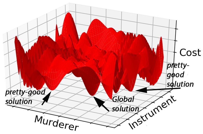
Table 1: Some Possible Reasons Why Mr. Boddy Keeps Getting Murdered

      He was mean.
      He was devastatingly handsome (or some trait that inspires envy/spite).
      He was burglarized.
      He was blackmailing the murderer for a large sum of money over a secret that the murderer does not want divulged.
      He witnessed a different murder and needed to be silenced.
      They were cases of mistaken identity.
      They were accidents.
      He was not murdered; he died naturally from his pre-existing asthmatic condition.

               P( xn+1 = −1) = f x (θmurder )
                                = f x ( P(instrument|location, P(instrument|murderer, P(instrument|reason,
                                                                                                                                    (3)
                                   P(murderer |location, P(murderer |reason, P(reason|location))))))).

Equation 3 reads: The probability that Mr. Boddy dies is a         appear simultaneously at one location.
function of the probability of instrument conditioned on loca-         To perform calculations, each distribution P(m|n) of
tion, conditioned on the probability of instrument conditioned     Equation 3 is written as an m × n × ( T + 1) matrix of
on murderer, conditioned on the probability of instrument con-     numbers in the range [0:1), where T is the number of
ditioned on reason, conditioned on the probability of murderer     time steps. These values are calculated directly from the
conditioned on location, conditioned on the probability of mur-    70-year record. For the new parameter values that we
derer conditioned on reason, conditioned on the probability of     added ourselves, we just assumed some statistics. We are
reason conditioned on location. No causality is assumed,           unable to justify this assumption, but shall wait through
and thus the ordering of these conditional probabilities           the prediction window to see whether it did any harm.
is arbitrary. Importantly, while the parameters θmurder                Finally, we examine the evolution of y, the unmea-
may in general be independent, they are not independent            sured level of IgE antibodies. Taking the case where
when a successful murder is pulled off. For example,               Mr. Boddy is alive at time n, yn+1 is governed by yn ,
if the instrument is a Mack Truck and the location is a            ythresh , and θasthma . If yn > ythresh , then at time (n + 1)
dining room, then a murder is unlikely to occur, because           Mr. Boddy dies and y will be reset to Mr. Boddy’s base-
it is nontrivial to squeeze a Mack Truck into most dining          line value. Otherwise yn+1 will depend on f y (θasthma ).
rooms. If a murder occurs and the murderer is blind,               The form of f y (θasthma ) is explained in a 27-page medical
the instrument is unlikely to be a Mack Truck. Also, for           pamphlet given to us by Mr. Boddy’s general practitioner,
a murder to occur the instrument and murderer must                 which is available upon request.

                                      III.   ESTIMATION AND PREDICTION

                     A. The problem                                    Generally, the model is written as:

                                                                              dx a (t)
                                                                                       = f a (x( t ), θ );   a = 1, 2, . . . , D,
                                                                                dt
Armed with observations and a model, we proceed to esti-
mation and prediction, using data assimilation. DA is an           which says what Equation 1 says for D = 2. Aside from
inverse formulation, whereby information contained in              the unknown parameters, the model is assumed to be
observations is harnessed to complete a model of the sys-          correct. In case that sounds foolish: it might be.
tem from which the observations were obtained, thereby                We seek to ascertain whether sufficient information
informing us of where the information came from [33].              can be propagated through the coupled equations dur-
In case that sounds like circular logic: it is not.                ing the window in which we have observations (the es-

                                                                                                                                     5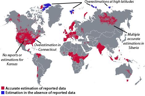
timation window) to estimate the parameters and the                           then the most probable path X given observations S is
dynamics of the unmeasured variables. The test of a                           the path that minimizes some quantity C. C we will treat
successful estimation is its ability to predict the model’s                   as a cost function to be minimized.
behavior in regions outside the window of observations -                          To calculate X0 9 , we need a useable form for C. To-
for example, the future7 .                                                    ward this end, let us rearrange and rewrite Equation 4,
                                                                              and for the moment focus on the observations (ignoring
                  B. The most likely hypothesis                               the model):
In this paper we use optimization to solve this inverse
problem. To scare up something to optimize, we define a                                C (X, S ) = − log P(X |S )
discretized state space in which our model lives. Within                                          = − ∑ CMI(x(n), s(n)|s(n − 1))
                                                                                                         n                                       (5)
the estimation window, this space is a ( D + Nθ )( T + 1)-
dimensional lattice, where Nθ is the number of parame-                                            = − ∑ MI(x(n)|s(n)).
                                                                                                         n
ters and T is the number of time steps. With D = 2, Nθ =
 Nθmurder + Nθasthma = 88 + 134, and T = 2, 207, 520, 001 for a
                                                                              On the second line of Equation Set 5, P(X |S ) is defined
step size of one second, the state space is 494,484,480,224-
                                                                              in terms of the conditional mutual information (CMI) [34]:
dimensional.
                                                                              the probability of the current state conditioned on the
      The series of lattice points that the model traverses
                                                                              current observation, conditioned on all previous observa-
during the estimation window is a path X. That
                                                                              tions. Next we assume that the observations at different
is, for our model, X = [x(t), θmurder (t), θ asthma (t)] =
                                                                              times are independent of each other, which is a ridiculous
[ x (t), y(t), θmurder (t), θ asthma (t)]. The path X defines the
                                                                              assumption, and which yields the simplified third line,
set of estimated values of all variables and parameters at
                                                                              involving the mutual information (MI) [35] between the
each timepoint that produced the observed deaths of Mr.
                                                                              state and the observation at time n.
Boddy within the 70-year history of observations.
      Now, some of the reported deaths include information                       Now let’s bring the model dynamics into the scheme.
regarding instrument, location, and/or murderer, while                        The Markov transition probabilities may contain errors,
some are incomplete. No reports include information                           and we add a second term to allow for that:
on reason or variable y. Not all events were necessarily
reported, and the time step between reports is variable                         C (X, S ) = − ∑ MI(x(n)|s(n)) − ∑ log[ P(Xn+1 |Xn ].
and typically larger than the time step of the dynamical
model evolution. In short, there exists much uncertainty                      Errors in the guess of initial conditions of the path should
- and consequently much wiggle room in defining a path                        also be considered, which would add a term − log[ P(x0 )].
that explains the data. In fact, there exists an infinite                     We, however, do not know the initial conditions. Thus
number of possible paths. We seek the path that is the                        we shall assume that the minimizing path is independent
one most likely to have produced the observations. This                       of initial conditions, and wait to see how egregiously this
most likely path is denoted X0 .                                              assumption impacts the prediction.
      How do we find path X0 ? The 494,484,480,224-                             Toward a useable form of C, we make two more
dimensional state space in which it lives is rather vo-                     ridiculous assumptions. First, both measurement and
luminous, and it would be a formidable task to define                       model errors have Gaussian distributions. That is, highly
the geometry of that space. Fortunately, we do not need                     improbable events probably will never happen (see Dis-
to know the shape of the space itself. We can define X0                     cussion). Second, there is no transfer function between
in terms of the observations and the dynamics.                              Mr. Boddy’s measured Alive-versus-Dead state versus
      Let us first consider how the observations, denoted                   his modeled Alive-versus-Dead state. Or: all accounts of
S = [st=0 , st=1 , ..., st=T ]8 , define X. If we write:                    occurrences of Dead are infinitely accurate and beyond
                         P(X |S ) = e−C(X,S ) ,                         (4) question. Finally, we write:
   7 Predictingthe past or the middle can also be fair game.
   8 Generally,the observations S consist of a set of sl distinct measured quantities. In our case we only observe one quantity: whether Mr.
Boddy is alive or dead. Thus, l = 1 and S can be simplified as written above.
  9 In addition to calculating the expectation value of X itself, we can calculate the expectation value of any known function G (X ) as:
              dXG (X )e−C(X,S )
           R
h G (X )i =    R
                 dXe−C(X,S )
                                .   That is, G (X ) is written as a weighted sum over all possible paths, with weights exponentially sensitive to C.

                                                                                                                                                  6
errormodel errorunitarity
errormeasurement z }| { z }| {
z }| {
N −1 D a N
A B
C= ∑ (s (n) − x a=1 (n))2 + ∑ ∑
2 l 2
( x a (n + 1) − f a (x(n), θ ))2 + λ ∑(| x a=1 (n)| − 1)2 , (6)
j n a n
where tn ≡ n, sl are measurements (or observations), x a routine will be continually updated and amended as new
are state variables, and θ are unknown parameters. The deaths are reported, to strengthen forecast accuracy.
coefficients A and B are inverse covariance matrices for
the measurement and model errors, respectively. In the E. The parameter search ranges and rare events
first term, a least-squares measurement error has been
As noted, taking as observations the 70-year reported his-
boiled down from mutual information. Only the variable
tory invites selection bias into the estimation procedure.
x is measured, and success of the estimation will required
Some reported deaths were poorly described, possibly
an efficient transfer of information from the measured
because the investigations were not seen to completion.
state x to unmeasured state y, as we require a completed
Further, not necessarily all deaths were reported. In ad-
model in order to generate predictions.
dition, even the complete reports appear to draw the
The second term of Equation 6 permits error in the
instrument, location, and murderer from rather rigid
model evolution - for example, stemming from the fact
boundary conditions. The location options, for example,
that the discretized state space does not have infinite res-
are nine rooms in a single house. This might be due to
olution. The third term is an equality constraint added
laziness on the part of the investigators, who didn’t feel
to impose unitarity: Mr. Boddy is never created or de-
stroyed, but rather is either alive or dead (but see Dis-
cussion on quantum effects). For a thorough derivation
leading from Equation 4 to 6, see Ref [36].
C. Estimation
The estimate of path X0 will consist of ( D + Nθ )( T +
1) = 494, 484, 480, 224 numbers. The search of the state
space for these numbers is performed via the variational
method [37], requiring that the first derivative of C with
respect to the minimizing path be zero, and that its sec-
ond derivate be positive-definite. The variational method
is descent-only, which presumes that the correct search
direction is always Downward. To avoid presuming this,
one may opt for Monte Carlos [38] instead.
If there exist degenerate solutions - for example, mul-
tiple explanations for a single crime - then finding the
minimizing path is nontrivial (Figure 4). To identify a
global minimum10 amid a sea of shallower minima, we
employ a method of iterative dart-throwing [39]. Figure 4: The surface of the cost function C: a
three-dimensional representation of the 494,484,480,224-
dimensional state space, with example directions murderer
D. Prediction and instrument. Top: The cost function is smooth and convex,
and thus there exists one global minimum corresponding to
Prediction involves taking as initial conditions the values the most likely path X0 . Bottom: A more realistic scenario [40]
of the variables and parameters11 at the final time step with multiple possibilities that may muddy the investigation.
of the estimation window, and integrating. The full DA
10 Actually, we don’t necessarily have to find the deepest minimum; we just need a minimum that is deep enough for our predictive
purposes. As we have yet to define our predictive purposes, perhaps the dart-throwing is premature.
11 The discriminating reader will wonder how we plan to integrate forward time-varying parameters with unknown dynamics. We have no
plan, and opt to ignore the problem. Thus we hope that the reader is not discriminating, and - by this Page 8 - has tired of reading footnotes.
7Table 2: Red Flags: Overestimates of Rare Events
It’s a serial killer.
It’s a serial killer with a different motive each time.
All murders were cases of mistaken identity*.
All murders were accidents.
Unlikely pairings of parameters occur, e.g. Dining Room and Mack Truck.
Any of the highly-unlikely parameter values (Figure 2) is overrepresented.
As the assumption of Gaussian-distributed errors will under-predict rare events, the overestimation of any of the above events
will be cause for concern. *Actually, we are not certain that the mistaken murder of Mr. Boddy 106 times is necessarily less
probable than the intentional murder of Mr. Boddy 106 times.
like extending their detective work outdoors. Indeed, values (see Figures 1 and 2, respectively, for examples).
some of what are typically considered highly likely loca- In addition, we added a few ludicrously-unlikely values,
tions, such as the Dark Alley or The Woods, may have such as the Asteroid, as a check on the DA procedure.
been undersampled. Moreover, we found that when our The assumption of Gaussian errors should under-predict
search ranges included only the reported parameter val- rare events, so if a ludicrously-unlikely event pops up
ues, estimates asymptoted to the bounds - a sign that the frequently in the estimation window, it is cause for con-
bounds needed extending. cern. Finally, some combinations of parameter values are
We extended the permitted values of all model param- particularly unlikely. For a list of some of these ”red
eters to include both highly-likely and highly-unlikely flags”, see Table 2.
IV. RESULT
Preliminary tests were performed using 80% of the time series of extremely rare events, namely: multiple
70-year time series as training data, with the remaining murders of one person.
20% reserved for prediction. These tests confirmed that The best estimations were those that omitted the
motive and asthma indeed are required for convergence. ludicrously-unlikely parameter values. Estimations for
They also indicated that the search ranges required ex- location, for example, are shown in Figure 5. Here, red
panding beyond their historically-defined values, as oth- and blue denote regions of correctly-estimated reported
erwise the estimates asymptoted to the bounds. These deaths, and erroneous estimations, respectively. The es-
preliminary tests marked one Lyapunov time12 at roughly timations over-all appear reasonable, and common loca-
a week. That is, the procedure stands a decent chance at tions pop up frequently. There are a few peculiarities,
predicting deaths through April 8. including erroneous estimations throughout the state of
As noted, we expanded the parameter search ranges Connecticut and on small islands near the Arctic circle.
to include ludicrously-unlikely values. In addition to In addition, we were surprised to note dense - and correct
providing a confidence check on the estimations, this - estimations in Siberia.
strategy was also intended to help distinguish between The prediction window for state variable x is shown
an historically unreported value because it wasn’t looked in Figure 6. For the Dead instances, circles and triangles
for, versus an unreported value because it is intrinsically represent murders and asthma attacks, respectively. The
rare. Unfortunately, expanding the search ranges to this first predicted regional event is: 17:19:03 EDT today, with
ludicrous extent increased the computational expense a standard deviation of seven hours, at The Kitchen at 4330
such that convergence failed. Thus, unfortunately we Katonah Avenue, Bronx, NY, 10470 (Figure 7), with either
were unable to probe the likelihoods of what arguably the Lead Pipe or the Lead Bust of Washington Irving.
are the most entertaining possibilities. Our assumption The motive is: Case of Mistaken Identity; there was no
of Gaussian errors may have precluded such findings convergence in the state space direction of murderer. The
anyway, although that assumption may in part be offset location is pinpointed quite accurately, which simplifies
by the fact that the procedure was trained upon an entire the next step: to test the result, we know where to go.
12 The Lyapunov time defines the characteristic timescale on which the dynamics of a system can be predicted (e.g. Ref [41]).
8Figure 5: Estimations of parameter location [42]. Noteworthy events are indicated. Red and blue denote correct and
erroneous estimations of death, respectively. Erroneous estimations occurred in Connecticut and on small islands near the
Arctic circle. Surprising dense reports from Siberia were estimated correctly.
Other events within the prediction window seem rea- Currently we are working to quantify the likelihood that
sonable. The Woods occurs often, in agreement with our either of these Texas reports represents the Nacogdoches
preconceived speculation that the Woods should occur prediction, given the error covariance between state x
often. Already we have confirmed the 3:10:59 event in and location.
Norway [43], which impressively was mere seconds off. Finally, the one disquieting prediction implicates the
Since 6am we have obtained off-the-books evidence of Woods on Tavira Island, Portugal. There are no woods on
two deaths in some woods in Northeastern Texas [44, 45]. Tavira Island, Portugal [46]. It is possible that, for some
Both are near the predicted 4:50:22 event in Nacogdoches.
Figure 6: Estimation and prediction window for the observed state variable x, with details given for some events. The
prediction window begins at 00:00:33 on April 1, and the next local event at 17:19:03 is denoted in bold. For Dead points, circles
and triangles represent murders and asthma attacks, respectively. *There are no woods on Tavira Island, Portugal; see text.
9local neighborhoods in the time series, location is a sloppy may be especially rapid in the direction of location. Exam-
direction in state space. In addition, this prediction oc- ining the model for specific locations of chaos, however,
curs later into the day, and the rate of divergence of paths is beyond the scope of this paper.
V. DISCUSSION
A. Who is/was Mr. Boddy? This might feel unsettling, but for a caveat: the time
resolution of reported deaths is one second at best. Thus,
While the estimation window overall appears reasonable,
the simultaneity of reports is questionable. At any rate,
there occurred a few peculiar events, including the er-
to grapple with them is beyond the scope of this paper.
roneous estimation in Connecticut and the prediction
in nonexistent woods on an island off Portugal. We
have acknowledged various assumptions throughout the C. The next murder: confirm or prevent?
modeling procedure, any of which may have introduced
Currently we are en route to The Bronx on the D train,
errors into the results. In particular, the assumption of
to await The Kitchen murder, and we recognize an ethi-
an over-simplistic model may be a problem.
cal dilemma: to attempt to prevent the murder? If we
We wrote Mr. Boddy’s internal dynamics solely in
intervene, we will impose an additional external force
terms of his binary alive-or-dead state and his IgE levels.
upon the dynamics, thereby altering the model. That is,
For future iterations of estimation we plan to flesh Mr.
to prevent the murder would preclude an assessment of
Boddy out a bit. For example, it might be useful to con-
the model’s predictive power. Meanwhile, in principle,
sider what kind of a human being he is/was. Aspects of
preventing the murder is the right thing to do [47]. We
his personality might yield insight into what he was up
note, however, the qualifier “in principle”, because in Mr.
to at The Kitchen in the Bronx, or in Siberia so frequently.
Boddy’s case murder does not appear to exert its charac-
Or, for that matter, in a nine-room mansion for 70 years.
teristic distasteful influence. Hm. Well, there remain a
few hours yet for soul-searching.
B. Quantum effects?
We’d like to address an apparent paradox in case it has
been noted by the reader. On one hand, quantum consid-
erations should not enter into the dynamical evolution
of a typically-sized human being wandering about the
planet at some typical rate of motion. For this reason we
imposed unitarity upon Mr. Boddy as a constraint in the
cost function. On the other hand, there has occurred a
handful of instances at which Mr. Boddy was reported to
be simultaneously alive and dead. Now, the formulation
of quantum mechanics indeed permits Mr. Boddy to
exist as a superposition of Alive and Dead states - until
he is observed. Here, we have allegations of simultaneous
observations of multiple state values. In other words, these Figure 7: Next local prediction: The Kitchen, Bronx, NY.
allegations belie quantum mechanics itself.
References
[1] Armstrong, Eve. Colonel Mustard in the Aviary with the Candlestick: a limit cycle attractor transitions to
a stable focus via supercritical Andronov-Hopf bifurcation. arXiv preprint arXiv:1803.11559, 2018.
[2] Abrams, Mrs. Betty. Miss Scarlett in the Dining Room with the Revolver. San Diego, California, 2018.
[3] Hasbro. Record of Sales, 2019.
10[4] Alfonsi, Alessandro. Professor Plum in the Library with the Rope. Positano, Italy, 2019.
[5] Pratt, Anthony E. Clue or Cluedo. Hasbro, Waddingtons, Parker Brothers, 1949.
[6] Betts, John T. Practical methods for optimal control and estimation using nonlinear programming, volume 19.
Siam, 2010.
[7] Evensen, Geir. Data assimilation: the ensemble Kalman filter. Springer Science & Business Media, 2009.
[8] Kalnay, Eugenia. Atmospheric modeling, data assimilation and predictability. Cambridge University Press,
2003.
[9] Kimura, Ryuji. Numerical weather prediction. Journal of Wind Engineering and Industrial Aerodynamics, 90(12-
15):1403–1414, 2002.
[10] Honegger, Milo. Shedding Light on Black Box Machine Learning Algorithms: Development of an Ax-
iomatic Framework to Assess the Quality of Methods that Explain Individual Predictions. arXiv preprint
arXiv:1808.05054, 2018.
[11] de Silva, Dr. Raymond. Diagnosis of severe eosinophilic asthma. Medical Records: Mr. Boddy, 2019.
[12] Sur, Sanjiv and Hunt, Loren W and Crotty, Thomas B and Gleich, Gerald J. Sudden-onset fatal asthma. In
Mayo Clinic Proceedings, volume 69, pages 495–496. Elsevier, 1994.
[13] Python, Full-grown Reticulated. https://www.activewild.com/reticulated-python-facts/. Accessed:
2019 Mar 24.
[14] Sondheim, Stephen & Hugh Wheeler. Sweeney Todd, the Demon Barber of Fleet Street - Original Broadway
Cast Recording. Dir: Harold Prince, Terry Hughes, 1979.
[15] Wife, The. Sarah White, this author’s sister, 2018.
[16] Cliff, The. https://www.38north.org/2018/04/gtoloraya041318/. Accessed: 2019 Mar 24.
[17] Scooter, The Electric. https://kid-krazy.com/products/300w-electric-scooter-pink-1?variant=
13053655679037&utm_campaign=gs-2018-07-30&utm_source=google&utm_medium=smart_campaign&gclid=
EAIaIQobChMI7Ovb2bqb4QIVGYnICh1iYAbgEAQYCCABEgLhjPD_BwE. Accessed: 2019 Mar 24.
[18] Chicken, Undercooked. https://www.featurepics.com/online/Roast-Chicken-2641205.aspx. Accessed:
2019 Mar 24.
[19] Alley, Dark. https://pixels.com/featured/dark-alley-octane-creative.html. Accessed: 2019 Mar 24.
[20] Woods, The. https://top-b.com/download_files/an-internal-communications-horror-story/
scary-woods/. Accessed: 2019 Mar 24.
[21] Baltimore. https://www.baltimoresun.com/news/maryland/baltimore-city/
bs-bz-baltimore-population-loss-jumps-20170322-story.html. Accessed: 2019 Mar 24.
[22] Carter, Jimmy. https://en.wikipedia.org/wiki/Jimmy_Carter. Accessed: 2019 Mar 24.
[23] Hook, Captain. https://pirates.fandom.com/wiki/James_Hook. Walt Disney Company. Accessed: 2019 Mar
24.
[24] Chicken, A. http://www.cubebreaker.com/these-are-10-of-the-weirdest-looking-chickens-youll-ever-see/
Accessed: 2019 Mar 24.
11[25] Dart, Poisoned. https://www.ldoceonline.com/Darts-topic/dart_2/,https://www.reddit.com/r/
flairwars/comments/956wi8/green_the_color_of_poison_not_life/. Accessed: 2019 Mar 24.
[26] Chair, Beanbag. https://www.bizchair.com/DG-BEAN-LARGE-SOLID-ROYBL-GG.html?gclid=
EAIaIQobChMIivzi3b2b4QIVTUsNCh32ZQBNEAQYAyABEgIPGPD_BwE. Accessed: 2019 Mar 24.
[27] Apple, Poisoned. https://www.reddit.com/r/flairwars/comments/956wi8/green_the_color_of_poison_
not_life/,https://www.yummyfruit.co.nz/. Accessed: 2019 Mar 24.
[28] Court, U.S. Supreme. https://www.supremecourt.gov/about/courtbuilding.aspx. Accessed: 2019 Mar 24.
[29] Mongolia. https://www.dailymail.co.uk/news/article-3582512/Incredible-photos-capture-harsh-reality-l
html. Accessed: 2019 Mar 24.
[30] Newsroom, CNN. https://www.cnn.com/2015/05/25/us/gallery/35-years-of-cnn/index.html. Accessed:
2019 Mar 24.
[31] Privault, Nicolas. Understanding Markov chains. Examples and Applications, Publisher Springer-Verlag Singapore,
2013.
[32] Bush, Robert K & Prochnau, Jay J. Alternaria-induced asthma. Journal of Allergy and Clinical Immunology,
113(2):227–234, 2004.
[33] Tarantola, Albert. Inverse problem theory and methods for model parameter estimation, volume 89. SIAM,
2005.
[34] Wyner, Aaron D. A definition of conditional mutual information for arbitrary ensembles. Information and
Control, 38(1):51–59, 1978.
[35] Cover, Thomas M & Thomas, Joy A. Elements of information theory. John Wiley & Sons, 2012.
[36] Abarbanel, Henry D.I. Predicting the future: completing models of observed complex systems. Springer, 2013.
[37] Smith, Donald R. Variational methods in optimization. Courier Corporation, 1998.
[38] Wong, Adrian S and Hao, Kangbo and Fang, Zheng and Abarbanel, Henry D.I. Precision Annealing
Monte Carlo Methods for Statistical Data Assimilation: Metropolis-Hastings Procedures. arXiv preprint
arXiv:1901.04598, 2019.
[39] Van Laarhoven, Peter JM & Aarts, Emile HL. Simulated annealing. In Simulated annealing: Theory and
applications, pages 7–15. Springer, 1987.
[40] Function, The Eggholder. http://www.sfu.ca/~ssurjano/egg.html. Accessed: 2019 Mar 24.
[41] Pikovsky, Arkady & Politi, Antonio. Lyapunov exponents: a tool to explore complex dynamics. Cambridge
University Press, 2016.
[42] World, The. https://pasarelapr.com/map/high-resolution-world-map-with-countries.html. Accessed:
2019 Mar 24.
[43] Yeager, Gretel. Private Communication, 2019.
[44] Undisclosed. Private Communication, 2019.
[45] Undisclosed. Private Communication, 2019.
[46] Tavira, Island Off Portugal. https://tavira.algarvetouristguide.com/beaches/tavira-island. Accessed:
2019 Mar 24.
[47] Bible, The. Ezekiel 33:8-9, 1200-165 B.C.
12You can also read