MC3D: Motion Contrast 3D Scanning
←
→
Page content transcription
If your browser does not render page correctly, please read the page content below
MC3D: Motion Contrast 3D Scanning
Nathan Matsuda Oliver Cossairt Mohit Gupta
Northwestern University Northwestern University Columbia University
Evanston, IL Evanston, IL New York, NY
Abstract
Structured light 3D scanning systems are fundamentally
constrained by limited sensor bandwidth and light source
power, hindering their performance in real-world appli-
cations where depth information is essential, such as in-
dustrial automation, autonomous transportation, robotic
surgery, and entertainment. We present a novel struc-
tured light technique called Motion Contrast 3D scanning
(MC3D) that maximizes bandwidth and light source power
to avoid performance trade-offs. The technique utilizes mo-
tion contrast cameras that sense temporal gradients asyn-
chronously, i.e., independently for each pixel, a property
that minimizes redundant sampling. This allows laser scan-
ning resolution with single-shot speed, even in the presence
of strong ambient illumination, significant inter-reflections,
and highly reflective surfaces. The proposed approach will
allow 3D vision systems to be deployed in challenging and
hitherto inaccessible real-world scenarios requiring high
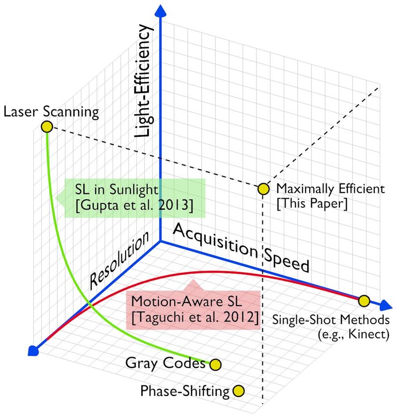
performance using limited power and bandwidth. Figure 1: Taxonomy of SL Systems: SL systems face trade-offs
in acquisition speed, resolution, and light efficiency. Laser scan-
1. Introduction ning (upper left) achieves high resolution at slow speeds. Single-
shot methods (mid-right) obtain lower resolution with a single
Many applications in science and industry, such as exposure. Other methods such as Gray coding and phase shift-
robotics, bioinformatics, augmented reality, and manufac- ing (mid-bottom) balance speed and resolution but have degraded
turing automation rely on capturing the 3D shape of scenes. performance in the presence of strong ambient light, scene inter-
Structured light (SL) methods, where the scene is actively reflections, and dense participating media. Hybrid techniques
illuminated to reveal 3D structure, provide the most accu- from Gupta et al. [16] (curve shown in green) and Taguchi et
rate shape recovery compared to passive or physical tech- al. [36] (curve shown in red) strike a balance between these ex-
tremes. This paper proposes a new SL method, motion contrast 3D
niques [7, 33]. Here we focus on triangulation-based SL
scanning (denoted by the point in the center), that simultaneously
techniques, which have been shown to produce the most ac-
achieves high resolution, low acquisition speed, and robust perfor-
curate depth information over short distances [34]. Most SL mance in exceptionally challenging 3D scanning environments.
systems operate with practical constraints on sensor band-
width and light source power. These resource limitations
force concessions in acquisition speed, resolution, and per-
formance in challenging 3D scanning conditions such as Speed-resolution trade-off in SL methods: Most existing
strong ambient light (e.g., outdoors) [25, 16], participat- SL methods achieve either high resolution or high acquisi-
ing media (e.g. fog, dust or rain) [19, 20, 26, 14], specu- tion speed, but not both. This trade-off arises due to lim-
lar materials [31, 27], and strong inter-reflections within the ited sensor bandwidth. On one extreme are the point/line
scene [15, 13, 11, 30, 4]. We propose a SL scanning ar- scanning systems [5] (Figure 1, upper left), which achieve
chitecture that overcomes these trade-offs by replacing the high quality results. However, each image captures only one
traditional camera with a differential motion contrast sensor point (or line) of depth information, thus requiring hundreds
to maximize light and bandwidth resource utilization. or thousands of images to capture the entire scene. Improve-
1
ments can be made in processing, such as the space-time                    sity (as the projected pattern varies) can achieve in-
analysis proposed by Curless et al. [12] to improve accu-                  variance to the scene’s BRDF.
racy and reflectance invariance, but ultimately traditional             Based on these observations, we present motion contrast 3D
point scanning remains a highly inefficient use of camera               scanning (MC3D), a technique that simultaneously achieves
bandwidth.                                                              the light concentration of light scanning methods, the speed
   Methods such as Gray coding [32] and phase shift-                    of single-shot methods, and a large dynamic range. The
ing [35, 15] improve bandwidth utilization but still re-                key idea is to use biologically inspired motion contrast sen-
quire capturing multiple images (Figure 1, lower center).               sors in conjunction with point light scanning. The pixels on
Single-shot methods [37, 38] enable depth acquisition (Fig-             motion contrast sensors measure temporal gradients of log-
ure 1, right) with a single image but achieve low resolu-               arithmic intensity independently and asynchronously. Due
tion results. Content-aware techniques improve resolution               to these features, for the first time, MC3D achieves high
in some cases [18, 23, 17], but at the cost of reduced cap-             quality results for scenes with strong specularities, signif-
ture speed [36]. This paper introduces a method achieving               icant ambient and indirect illumination, and near real-time
higher scan speeds while retaining the advantages of tradi-             capture rates.
tional laser scanning.
                                                                        Hardware prototype and practical implications: We
Speed-robustness trade-off: This trade-off arises due to                have implemented a prototype MC3D system using off the
limited light source power and is depicted by the green SL              shelf components. We show high quality 3D scanning re-
in sunlight curve in Figure 1. Laser scanning systems con-              sults achieved using a single measurement per pixel, as well
centrate the available light source power in a smaller region,          as robust 3D scanning results in the presence of strong am-
resulting in a large signal-to-noise ratio, but require long            bient light, significant inter-reflections, and highly specular
acquisition times. In comparison, the full-frame methods                surfaces. We establish the merit of the proposed approach
(phase-shifting, Gray codes, single-shot methods) achieve               by comparing with existing systems such as Kinect 2 , and
high speed by illuminating the entire scene at once but are             binary SL. Due to its simplicity and low-cost, we believe
prone to errors due to ambient illumination [16] and indirect           that MC3D will allow 3D vision systems to be deployed
illumination due to inter-reflections and scattering [13].              in challenging and hitherto inaccessible real-world scenar-
Limited dynamic range of the sensor: For scenes com-                    ios which require high performance with limited power and
posed of highly specular materials such as metals, the dy-              bandwidth.
namic range of the sensor is often not sufficient to capture
the intensity variations of the scene. This often results in            2. Ambient and Global Illumination in SL
large errors in the recovered shape. Mitigating this chal-
lenge requires using special optical elements [27] or captur-               SL systems rely on the assumption that light travels di-
ing a large number of images [31].                                      rectly from source to scene to camera. However, in real-
                                                                        world scenarios, scenes invariably receive light indirectly
Motion contrast 3D scanning: In order to overcome these                 due to inter-reflections and scattering, as well as from am-
trade-offs and challenges, we make the following three ob-              bient light sources (e.g., sun in outdoor settings). In the
servations:                                                             following, we discuss how point scanning systems are the
  Observation 1: In order for the light source to be used               most robust in the presence of these undesired sources of
  with maximum efficiency, it should be concentrated on                 illumination.
  the smallest possible scene area. Point light scanning                Point scanning and ambient illumination. Let the scene
  systems concentrate the available light into a single                 be illuminated by the structured light source and an ambient
  point, thus maximizing SNR.                                           light source. Full-frame SL methods (e.g., phase-shifting,
  Observation 2: In conventional scanning based SL                      Gray coding) spread the power of the structured light source
  systems, most of the sensor bandwidth is not utilized.                over the entire scene. Suppose the brightness of the scene
  For example, in point light scanning systems, every                   point due to the structured light source and ambient illumi-
  captured image has only one sensor pixel 1 that wit-                  nation are P and A, respectively. Since ambient illumina-
  nesses an illuminated spot.                                           tion contributes to photon noise, the SNR of the intensity
                                                                        measurement can be approximated as √PA [16]. However, if
  Observation 3: If materials with highly specular                      the power of the structured light source is concentrated into
  BRDFs are present, the range of intensities in the scene              only a fraction of the scene at a time, the effective source
  often exceed the sensor’s dynamic range. However,                     power increases and higher SNR is achieved. We refer to
  instead of capturing absolute intensities, a sensor that
  captures the temporal gradients of logarithmic inten-                    2 We compare with the first-generation Kinect, which uses active tri-

                                                                        angulation depth recovery, instead of the new Kinect, which is based on
  1 Assuming   the sensor and source spatial resolutions are matched.   Time-of-Flight.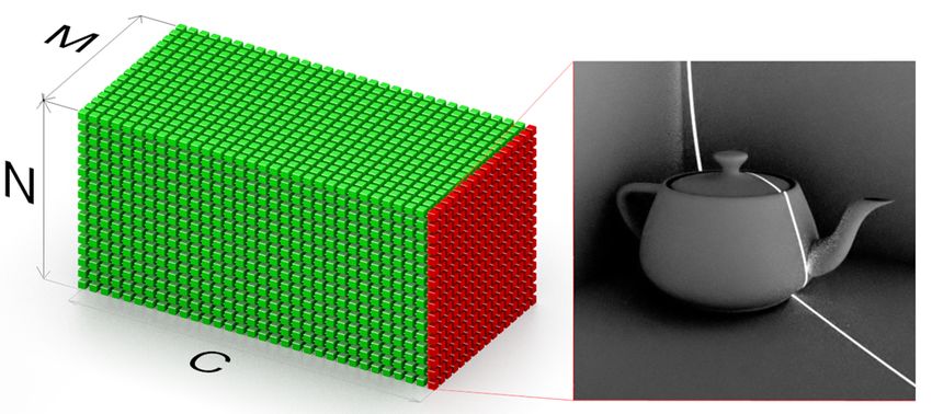
SDE              LCR
   Point Scan        R×C               1
   Line Scan           C              1/R
     Binary       log(C) + 2     1/(R×C)
 Phase Shifting        3         1/(R×C)
  Single-Shot          1         1/(R×C)
                                                 (a) Line Scan         (b) Binary SL        (c) Phase Shift       (d) Single-Shot
Figure 2: SL methods characterized by SPD and LER: (a) Line scanning captures all disparity measurements in C images. (b) Binary
patterns reduce the images to log2 (C) + 2. (c) Phase shifting needs a minimum of three sinusoidal patterns. (d) Single-shot methods
require only a single exposure but make smoothness assumptions that reduces resolution.

this fraction as the Light Concentration Ratio (LCR). The           requirement than Equation 2, point scanning systems are
                               P√
resulting SNR is given as LCR     A
                                    . Since point scanning          much more robust in the presence of significant global illu-
systems maximally concentrate the light (into a single scene        mination (e.g. a denser T matrix).
point), they achieve the minimum LCR and produce the                Sampling efficiency: While point scanning produces opti-
most robust performance in the presence of ambient illumi-          mal performance in the presence of ambient and global il-
nation for any SL system.                                           lumination, it is an extremely inefficient sampling strategy.
Point scanning and global illumination. The contribu-               We define the sampling efficiency in terms of the number
tions of both direct and indirect illumination may be mod-          of pixel samples required per depth estimate (SDE). Ide-
eled by the light transport matrix T that maps a set of R ×C        ally, we want SDE = 1, but conventional point scanning
projected intensities p from a projector onto the M × N             (as well as several other SL methods) captures many images
measured intensities c from the camera.                             for estimating depth, thus resulting in SDE > 1.

                           c = T p.                        (1)      2.1. SDE and LCR of Existing Methods
The component of light that is directly reflected to the ith            Figure 2 compares SDE and LCR values for existing
camera pixel is given by Ti,α pα where the index α de-              SL methods. We consider Point Scan, Line Scan (Fig-
pends on the depth/disparity of the scene point. All other          ure 2a), Binary SL/ Gray coding (Figure 2b), Phase Shifted
entries of T correspond to contributions from indirect re-          SL (Figure 2c), and Single-shot SL (Figure 2d). Scanning
flections, which may be caused by scene inter-reflections,          methods have small LCR but require numerous image cap-
sub-surface scattering, or scattering from participating me-        tures, resulting in a larger SDE. Binary SL, Phase Shifted
dia. SL systems project a set of K patterns which are used          SL, and Single-shot methods require fewer images, but this
to infer the index α that establishes projector-camera cor-         is achieved by increasing LCR for each frame.
respondence. For SL techniques that illuminate the entire           Hybrid methods: Hybrid techniques can achieve higher
scene at once, such as phase-shifting SL and binary SL, the         performance by adapting to scene content. Motion-aware
sufficient condition for estimating α is that direct reflection     SL, for example, uses motion analysis to reallocate band-
must be greater than the sum of all indirect contributions:         width for either increased resolution or lower acquisition
                              X                                     time given a fixed SDE [36]. A recent approach [16] pro-
                      Ti,α >       Ti,k .                   (2)     poses to increase LCR in high ambient lighting by increas-
                               k6=α
                                                                    ing SDE. Hybrid methods aim to prioritize the allocation
For scenes with significant global illumination, this condi-        of LCR and SDE depending on scene content and imag-
tion is often violated, resulting in depth errors [13]. For         ing conditions, but are still subject to the same trade-offs as
point scanning, a set of K = R × C images are captured,             the basic SL methods.
each corresponding to a different column ti of the matrix
T . In this case, a sufficient condition to estimate α is sim-      2.2. The Ideal SL System
ply that direct reflection must be greater than each of the
individual indirect sources of light, i.e:                             An ideal SL system maximizes both bandwidth and light
                                                                    source usage as follows:
        Ti,α > Ti,k , ∀k ∈ {1, · · · R × C}, k 6= α.       (3)
                                                                       Definition 1 A Maximally Efficient SL System
If this condition is met, α can be found by simply thresh-             satisfies the constraint:
olding each column ti such that only one component re-
mains. Since Equation 3 is a significantly less restrictive                        SDE = 1, LCR = 1/(R × C)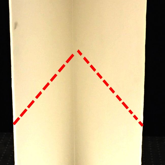
(a) Conventional Camera                                            (b) Motion Contrast Camera
Figure 3: Conventional vs. Motion Contrast Output: (a) The space-time volume output of a conventional camera consists of a series of
discrete full frame images (here a black circle on a pendulum). (b) The output of a motion contrast camera for the same scene consists of a
small number of pixel change events scattered in time and space. The sampling rate along the time axis in both cameras is limited by the
camera bandwidth. The sampling rate for motion contrast is far higher because of the naturally sparse distribution of pixel change events.

Intuitively, LCR = 1/(R × C) implies the use of point                   parts of the image. For a scanning SL system, this wasted
scanned illumination, i.e., the structured illumination is              bandwidth contains measurements that provide no depth es-
concentrated into one scene point at a time. On the other               timates, raising the SDE of the system. The motion con-
hand, SDE = 1 means that each scene point is sampled                    trast camera only makes measurements at points that are
only once, suggesting a single-shot method. Unfortunately,              illuminated by the scanned light, enabling a SDE of 1.
scanned illumination methods have low SDE and single-                       For our prototype, we use the iniLabs DVS128 [24]. The
shot methods have low LCR. How can a system be both                     camera module contains a 1st generation 128x128 CMOS
single-shot and scanning?                                               motion contrast sensor, which has been used in research
    We reconcile this conflict by revisiting our observation            applications such as high frequency tracking [28], unsu-
that illumination scanning systems severely under-utilize               pervised feature extraction [8], and neurologically-inspired
camera bandwidth. Ideally, we need a sensor that measures               robotic control systems [21]. This camera has also been
only the scene points that are illuminated by the scanning              used to recover depth by imaging the profile of a fixed-
light source. Although conventional sensors do not have                 position, pulsed laser in the context of terrain mapping [9].
such a capability, we draw motivation from biological vi-                   The DVS128 uses event time-stamps assigned using a
sion where sensors that only report salient information are             100kHz counter [24]. For our 128 pixel line scanning setup
commonplace. Organic photoreceptors respond to changes                  this translates to a maximum resolvable scan rate of nearly
in instantaneous contrast, implicitly culling static informa-           800Hz. The dynamic range of the DVS is more than 120dB
tion. If such a sensor observes a scene lit with scanning               due to the static background rejection discussed earlier [24].
illumination, measurement events will only occur at scene
points containing the moving spot. Digital sensors mimick-              4. Motion Contrast 3D Scanning
ing the differential nature of biological photoreceptors are
now available as commercially packaged camera modules.                      We now present Motion Contrast 3D scanning (MC3D).
Thus, we can use these off-the-shelf components to build a              The key principle behind MC3D is the conversion of spatial
scanning system that utilizes both light power and measure-             projector-camera disparity to temporal events recorded by
ment bandwidth in the maximally efficient manner.                       the motion contrast sensor. Interestingly, the idea of map-
                                                                        ping disparity to time has been explored previously in the
3. Motion Contrast Cameras                                              VLSI community, where several researchers have devel-
                                                                        oped highly customized CMOS sensors with on-pixel cir-
   Lichtsteiner et al. [24] recently introduced the biologi-            cuits that record the time of maximum intensity [6, 22, 29].
cally inspired Motion Contrast Camera, in which pixels on               The use of a motion contrast sensor in a 3D scanning system
the sensor independently and asynchronously generate out-               is similar to these previous approaches with two important
put when they observe a temporal intensity gradient. When               differences: 1) The differential logarithmic nature of motion
plotted in x, y, and time, the motion contrast output stream            contrast cameras improves performance in the presence of
appears as a sparse distribution of discrete events corre-              ambient illumination and arbitrary scene reflectance, and 2)
sponding to individual pixel changes. Figure 3b depicts the             motion contrast cameras are currently commercially avail-
output of a motion contrast camera when viewing a black                 able while previous techniques required custom VLSI fabri-
circle attached to a pendulum swinging over a white back-               cation, limiting access to only the small number of research
ground. Note that the conventional camera view of this ac-              labs with the requisite expertise.
tion, shown in Figure 3a, samples slowly along the time                     MC3D consists of a laser line scanner that is swept rela-
axis to account for bandwidth consumed by the non-moving                tive to a DVS sensor. The event timing from the DVS is used
Projector-Camera Geometry                                       Sensor Events                                        Projector-Camera Correspondences
                             s2
                                                          [ i 1 ,τ1 ] [ i 2 ,τ2 ]

                                                                                                 Projector Position
                                                                                                                      j2

                                           Event Output

                                                                                                    (estimated)
               t2       s1
                                                                                                                      j1
       α2             t1
               α1 i i2                                         t1         t2         Time
                                                                                                                                 τ1     τ2      Event Time
                   1
   Projector        Camera

Figure 4: System Model: A scanning source illuminates projector positions α1 and α2 at times t1 and t2 , striking scene points s1 and
s2 . Correspondence between projector and camera coordinates is not known at runtime. The DVS sensor registers changing pixels at
columns i1 and i2 at times t1 and t2 , which are output as events containing the location/event time pairs [i1 , τ1 ] and [i2 , τ2 ]. We recover
the estimated projector positions j1 and j2 from the event times. Depth can then be calculated using the correspondence between event
location and estimated projector location.

to determine scan angle, establishing projector-camera cor-
respondence for each pixel. The DVS was used previously
                                                                                                     cM  C
                                                                                                      i,t = log(ci,t ) − log(ci,t+1 ),           (6)
for SL scanning by Brandli et al. [9] in a pushbroom setup
that sweeps an affixed camera-projector module across the                                                          I0 + Ib
                                                                                                           = log              δα,t .             (7)
scene. This technique is useful for large area terrain map-                                                           Ib
ping but ineffective for 3D scanning of dynamic scenes. Our                           Next, the motion contrast intensity is thresholded and the set
focus is to design a SL system capable of 3D capture for ex-                          of space and time indices are transmitted asynchronously as
ceptionally challenging scenes, including those containing                            tuples:
fast dynamics, significant specularities, and strong ambient
                                                                                                    [i, τ ], s.t. cM  C
                                                                                                                   i,t > , τ = t + σ,         (8)
and global illumination.
   For ease of explanation, we assume that the MC3D sys-                              where σ is the timing noise that may be present due to pixel
tem is free of distortion, blurring, and aberration; that the                         latency, multiple event firings, and projector timing drift.
projector and camera are rectified and have equal focal                               The tuples are transmitted as an asynchronous stream of
lengths f ; and are separated by a baseline b 3 . We use a 1D                         events (Figure 4 middle) which establish correspondences
analysis that applies equally to all camera-projector rows.                           between camera columns i and projector columns j = τ · S
A scene point s = (x, z) maps to column i in the camera                               (Figure 4 right), where S is the projector scan speed in
image and the corresponding column α in the projector im-                             columns/sec. The depth is then calculated as:
age (see Figure 4). Referring to the right side of Equation 1,                                                         bf
after discretizing time by the index t the set of K = R × C                                                             z(i) =.              (9)
                                                                                                                  (i − τ · S)
projected patterns from a point scanner becomes:                                      Fundamentally, MC3D is a scanning system, but it dif-
                                                                                      fers from conventional implementations because the motion
                    P = [p1 , · · · pK ] = I0 δi,t + Ib ,                      (4)    contrast sensor implicitly culls unnecessary measurements.
                                                                                      A conventional camera must sample the entire image for
where δ is the Kronecker delta function, I0 is the power of
                                                                                      each scanned point (see Figure 5a), while the motion con-
the focused laser beam, and Ib represents the small amount
                                                                                      trast camera samples only one pixel, drastically reducing
of background illumination introduced by the projector (e.g.
                                                                                      the number of measurements required (see Figure 5b).
due to scattering in the scanning optics). From Equation 1,
the light intensity directly reflected to the camera is:                              Independence to scene reflectivity. A closer look at Equa-
                                                                                      tions 5 and 7 reveal that while the intensity recorded by
               ci,t = Ti,α Pα,t = (I0 δα,t + Ib )Ti,α ,                        (5)    a conventional laser scanning system depends on scene re-
                                                                                      flectivity, MC3D does not. Strictly speaking, the equation
where Ti,α denotes the fraction of light reflected in direc-                          only takes direct reflection into account, but BRDF invari-
tion i that was incident in direction α (i.e. the BRDF) and                           ance still holds approximately when ambient and global il-
the pair [i, α] represent a projector-camera correspondence.                          lumination are present. This feature, in combination with
Motion contrast cameras sense the time derivative of the                              the logarithmic response, establishes MC3D as a much
logarithm of incident intensity [24]:                                                 more robust technique for estimating depth of highly reflec-
    3 Lack of distortion, equal focal lengths, etc., are not a requirement for        tive objects, as demonstrated by the experiments shown in
the system and can be accounted for by calibration.                                   Figure 9.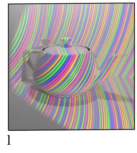
at 500 mm from the sensor, depth error was 12.680 mm
                                                                     RMSE. In both cases, SDE = 1 and LCR = 1/(R × C)
                                                                     and the SHOWWX projector was used as the source.
                                                                     Evaluation of complex scenes: To demonstrate the advan-
                                                                     tages of our system in more realistic situations, we used
                                                                     two test objects: a medical model of a heart and a miniature
                                                                     plaster bust. These objects both contain smooth surfaces,
                                                                     fine details, and strong silhouette edges.
                                                                         We captured these objects with our system and the Mi-
                    (a) Conventional Camera
                                                                     crosoft Kinect depth camera [1]. The Kinect is based on
                                                                     a single-shot scanning method and has a similar form fac-
                                                                     tor and equivalent field of view when cropped to the same
                                                                     resolution as our prototype system. For our experimental
                                                                     results, we captured test objects with both systems at iden-
                                                                     tical distances and lighting conditions. We fixed the expo-
                                                                     sure time for both systems at 1 second, averaging all input
                                                                     data during that time to produce a single disparity map. We
                  (b) Motion Contrast Camera                         applied a 3x3 median filter to the output of both systems.
                                                                     The resulting scans, shown in Figure 6, clearly show in-
Figure 5: Traditional vs. MC3D Line Scanning: (a) A tradi-           creased fidelity in our system as compared to the Kinect.
tional camera capturing C scanned lines will require M ×N ×C
                                                                     The SHOWWX projector was used as the source in these
samples for a single scan. The camera data is reported in the form
                                                                     experiments.
of 2D intensity images. (b) A motion contrast camera only reports
information for each projected line and uses a bandwidth of just         We also captured the same scenes with traditional laser
M ×C per scan. The motion contrast output consists of an x, y,       scanning using the same galvanometer setup and an IDS
time triplet for each sample.                                        UI348xCP-M Monochrome CMOS camera. The image was
                                                                     cropped using the camera’s hardware region of interest to
5. Experimental Methods and Results                                  128x128. The camera was then set to the highest possible
                                                                     frame rate at that resolution, or 573fps. This corresponds to
DVS operation: In our system, DVS sensor parameters are              a total exposure time of 28.5s, though the real world capture
set via a USB interface. In all our experiments, we maxi-            time was 22 minutes. Note that MC3D, while requiring sev-
mized the built-in event rate cap to use all available band-         eral orders of magnitude less capture time than traditional
width and maximized the event threshold  to reject extra-           laser scanning, achieves similar quality results.
neous events.
                                                                     Ambient lighting comparison: Figure 7 shows the perfor-
Light source: We used two different sources in our pro-
                                                                     mance of our system under bright ambient lighting condi-
totype implementation: a portable, fixed-frequency point
                                                                     tions as compared to Kinect. We floodlit the scene with a
scanner and a variable-frequency line scanner. The portable
                                                                     broadband halogen lamp whose emission extends well into
scanner was a SHOWWX laser pico-projector from Mi-
                                                                     the infrared region used by the Kinect sensor. The ambient
crovision, which displays VGA input at 848x480 60Hz by
                                                                     intensity was controlled by adjusting the lamp distance from
scanning red, green, and blue laser diodes with a MEMS mi-
                                                                     the scene. Errors in the Kinect disparity map become signif-
cromirror [2]. The micromirror follows a traditional raster
                                                                     icant even for small amounts of ambient illumination as has
pattern, thus functioning as a self-contained 60Hz laser spot
                                                                     been shown previously [10]. In contrast, MC3D achieves
scanner. For the variable-frequency line scanner, we used
                                                                     high quality results for a significantly wider range of ambi-
a Thorlabs GVSM002 galvanometer coupled with a Thor-
                                                                     ent illumination. The illuminance of the laser pico-projector
labs HNL210-L 21mW HeNe Laser and a cylindrical lens.
                                                                     used in this experiment is around 150 lux, measured at the
The galvanometer is able to operate at scan speeds from 0-
                                                                     object. MC3D performs well under ambient flux an order of
250Hz.
                                                                     magnitude above that of the projector. The SHOWWX pro-
Evaluation of simple shapes: To quantitatively evaluate              jector was used as the source in these experiments, which
the performance of our system, we scanned a plane and a              has a listed laser power of 1mW. The Kinect, according to
sphere. We placed the plane parallel to the sensor at a dis-         the hardware teardown at [3], has a 60mW laser source. The
tance of 500 mm and captured a single scan (one measure-             Kinect is targeted at indoor, eye-safe usage, but our exper-
ment per pixel). Fitting an analytic plane to the result us-         imental setup nonetheless outperforms the Kinect ambient
ing least squares, we calculated a depth error of 7.849 mm           light rejection at even lower power levels due to the light
RMSE. Similarly, for a 100 mm diameter sphere centered               concentration advantage of laser scanning.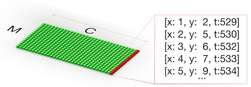
(a) Reference Photo                (b) Laser Scan                      (c) Kinect                      (d) MC3D

         (e) Reference Photo                 (f) Laser Scan                      (g) Kinect                    (h) MC3D
Figure 6: Comparison with Laser Scanning and Microsoft Kinect: Laser scanning performed with laser galvanometer and traditional
sensor cropped to 128x128 with total exposure time of 28.5s. Kinect and MC3D methods captured with 1 second exposure at 128x128
resolution (Kinect output cropped to match) and median filtered. Object placed 1m from sensor under ∼150 lux ambient illuminance
measured at object. Note that while the image-space resolution for all 3 methods are matched, MC3D produces depth resolution equivalent
to laser scanning, whereas the Kinect depth is more coarsely quantized.

Strong scene inter-reflections: Figure 8 shows the per-               ential motion contrast, it is more robust for scenes with a
formance of MC3D for a scene with significant inter-                  wide dynamic range. As shown in the cross-section plot
reflections. The test scene consists of two pieces of white           on the right, MC3D faithfully recovers the spherical sur-
foam board meeting at a 30 degree angle. The scene pro-               face while Gray coding SL produces significant errors at
duces significant inter-reflections when illuminated by a             the boundary and center of the sphere.
SL source. As shown in the cross-section plot on the
right, MC3D faithfully recovers the V-groove of the two               Motion comparison: We captured a spinning paper pin-
boards while Gray coding SL produces significant errors               wheel using the SHOWWX projector to show the system’s
that grossly misrepresent the shape. The galvanometer line            high rate of capture. Four frames from this motion se-
scanner was used as the source in these experiments.                  quence are shown at the top of Figure 10. Each image cor-
                                                                      responds to consecutive 16ms exposures captured sequen-
Specular materials: Figure 9 shows the performance of                 tially at 60fps. A Kinect capture at the bottom of the figure
MC3D for a highly specular steel sphere using the gal-                shows the pinwheel captured at the maximum 30fps frame
vanometer line scanner. The reflective appearance produces            rate of that sensor.
a wide dynamic range that is particularly challenging for
conventional SL techniques. Because MC3D senses differ-
Photo
                                                                                                      - Gray
                                                                                                      - MC3D

                            MC3D

                            Kinect
                                                                              Setup                        Depth Profile
                                                                   Figure 9: Performance with Reflective Surfaces: The image on
                                                                   the left depicts a reflective test scene consisting of a shiny steel
  (a) 150lux (b) 500lux (c) 1000lux (d) 2000lux (e) 5000lux        sphere. The plot on the right shows the depth output from Gray
                                                                   coding and MC3D. Both scans were captured with an exposure
Figure 7: Output Under Ambient Illumination: Disparity out-        time of 1/30th second. The Gray coding method used 22 consec-
put for both methods captured with 1 second exposure at 128x128    utive coded frames, while MC3D results were averaged over 22
resolution (Kinect output cropped to match) under increasing il-   frames. The Gray code output produces significant artifacts not
lumination from 150 lux to 5000 lux measured at middle of the      present in MC3D output.
sphere surface. The illuminance from our projector pattern was
measured at 150lux. Note that in addition to outperforming the
Kinect, MC3D returns usable data at ambient illuminance levels
an order of magnitude higher than the projector power.

                                  - Gray
                                  - MC3D                                                       (a) MC3D

                                                                                              (b) Kinect
                                                                   Figure 10: Motion Comparison: The top row depicts 4 frames of
         Setup                         Depth Profile               a pinwheel spinning at roughly 120rpm, captured at 60fps using
                                                                   MC3D. The bottom row depicts the same pinwheel spinning at the
Figure 8: Performance with Interreflections: The image on the      same rate, over the same time interval captured with the Kinect.
left depicts a test scene consisting of two pieces of white foam   Only 2 frames are shown due to the 30fps native frame rate of the
board meeting at a 30 degree angle. The middle row of the depth    Kinect. Please see movies of our real-time 3D scans in Supple-
output from Gray coding and MC3D are shown in the plot on the      mentary Materials.
right. Both scans were captured with an exposure time of 1/30th
second. Gray coding used 22 consecutive coded frames, while
MC3D results were averaged over 22 frames. MC3D faithfully
                                                                   Kinect and Gray coding, it falls short of achieving laser scan
recovers the V-groove shape while the Gray code output contains
                                                                   quality. This is mostly due to the relatively small resolution
gross errors.
                                                                   (128 × 128) of the DVS and is not a fundamental limita-
                                                                   tion. The DVS used in our experiments is the first com-
6. Discussion and Limitations                                      mercially available motion contrast sensor. Subsequent ver-
                                                                   sions are expected to achieve higher resolution, which will
   We have introduced MC3D, a new approach to SL that              enhance the quality of the results achieved by our technique.
eliminates redundant sampling of irrelevant pixels and max-        Furthermore, we intend to investigate superresolution tech-
imizes laser scanning speed. This arrangement retains the          niques to improve spatial resolution.
light efficiency and resolution advantages of laser scan-             There are several noise sources in our prototype system
ning while attaining the real-time performance of single-          such as uncertainty in event timing due to internal electri-
shot methods.                                                      cal characteristics of the sensor, multiple event firings dur-
   While our prototype system compares favorably against           ing one brightness change event, or downsampling in the
Disparity Maps References
[1] Microsoft Kinect. http://www.xbox.com/kinect. 6
[2] Microvision SHOWWX. https://web.archive.
org/web/20110614205539/http://www.
microvision.com/showwx/pdfs/showwx_
userguide.pdf. 6
[3] Openkinect hardware info. http://openkinect.org/
1 Hz 30 Hz 250 Hz wiki/Hardware_info. 6
Valid Pixels vs Capture Rate
Stddev Valid Pixels (disparity)
Performance vs Capture Rate [4] S. Achar and S. G. Narasimhan. Multi Focus Structured
100 5.4
5.2
Light for Recovering Scene Shape and Global Illumination.
90 5 In ECCV, 2014. 1
Valid Pixels (%)
4.8
80 [5] G. J. Agin and T. O. Binford. Computer description of curved
4.6
70 4.4 objects. IEEE Transactions on Computers, 25(4), 1976. 1
4.2
60 4 [6] K. Araki, Y. Sato, and S. Parthasarathy. High speed
3.8 rangefinder. In Robotics and IECON’87 Conferences, pages
50
3. 6
40 3.4
184–188. International Society for Optics and Photonics,
0 50 100 150 200 250 0 50 100 150 200 250 1988. 4
Capture Rate (Hz) Capture Rate(Hz)
[7] P. Besl. Active, optical range imaging sensors. Machine
vision and applications, 1(2), 1988. 1
Figure 11: MC3D Performance vs Scan Rates: The row of im-
[8] O. Bichler, D. Querlioz, S. J. Thorpe, J.-P. Bourgoin, and
ages depict the disparity output from a single sweep of the laser
C. Gamrat. Unsupervised features extraction from asyn-
at 1hz, 30hz, and 250hz. Bottom left, the number of valid pixels
chronous silicon retina through spike-timing-dependent plas-
recovered on average for one scan at different scan rates decreases
ticity. Neural Networks (IJCNN), International Joint Confer-
with increasing scan frequency. Bottom right, the standard devia-
ence on, 2011. 4
tion of the depth map increases with increasing scan frequency.
[9] C. Brandli, T. A. Mantel, M. Hutter, M. A. Höpflinger,
sensors digital interface. The trade-off between noise and R. Berner, R. Siegwart, and T. Delbruck. Adaptive pulsed
laser line extraction for terrain reconstruction using a dy-
scan speed is investigated in Figure 11. As scan speed
namic vision sensor. Frontiers in neuroscience, 7, 2013. 4,
increases, timing errors are amplified, resulting in an in- 5
creased amount of dropped events (bottom-left), which de-
[10] D. Castro and Mathur. Kinect outdoors. www.youtube.
grades the quality of recovered depth maps (bottom-right). com/watch?v=rI6CU9aRDIo. 6
These can be mitigated through updated sensor designs, fur- [11] V. Couture, N. Martin, and S. Roy. Unstructured light scan-
ther system engineering, and more sophisticated point cloud ning robust to indirect illumination and depth discontinuities.
processing. We plan to provide a thorough noise analysis in IJCV, 108(3), 2014. 1
a future publication. [12] B. Curless and M. Levoy. Better optical triangulation
Despite limitations, our hardware prototype shows that through spacetime analysis. In IEEE ICCV, 1995. 2
this method can be implemented using off-the-shelf com- [13] M. Gupta, A. Agrawal, A. Veeraraghavan, and S. G.
ponents with minimal system integration. The results from Narasimhan. A practical approach to 3D scanning in the
this prototype show promise in outperforming existing com- presence of interre.ections, subsurface scattering and defo-
mercial single-shot SL systems, especially in terms of both cus. IJCV, 102(1-3), 2012. 1, 2, 3
speed and performance. Improvements are necessary to [14] M. Gupta, S. G. Narasimhan, and Y. Y. Schechner. On con-
develop single-shot laser scanning into a commercially vi- trolling light transport in poor visibility environments. In
able product, but nonetheless our simple prototype demon- IEEE CVPR, pages 1–8, June 2008. 1
strates that the MC3D concept has clear benefits over exist- [15] M. Gupta and S. K. Nayar. Micro phase shifting. IEEE
ing methods for dynamic scenes, highly specular materials, CVPR, 2012. 1, 2
and strong ambient or global illumination. [16] M. Gupta, Q. Yin, and S. K. Nayar. Structured light in sun-
light. IEEE ICCV, 2013. 1, 2, 3
[17] K. Hattori and Y. Sato. Pattern shift rangefinding for accurate
7. Acknowledgments shape information. MVA, 1996. 2
[18] E. Horn and N. Kiryati. Toward optimal structured light pat-
This work was supported by funding through the Bi- terns. Image and Vision Computing, 17(2), 1999. 2
ological Systems Science Division, Office of Biological [19] J. S. Jaffe. Computer modeling and the design of optimal
and Environmental Research, Office of Science, U.S. Dept. underwater imaging systems. IEEE Journal of Oceanic En-
of Energy, under Contract DE-AC02-06CH11357. Addi- gineering, 15(2), 1990. 1
tionally, this work was supported by ONR award number [20] J. S. Jaffe. Enhanced extended range underwater imaging via
1(GG010550)//N00014-14-1-0741. structured illumination. Optics Express, (12), 2010. 1
[21] A. Jimenez-Fernandez, J. L. Fuentes-del Bosh, R. Paz-
     Vicente, A. Linares-Barranco, and G. Jimenez. Neuro-
     inspired system for real-time vision sensor tilt correction. In
     IEEE ISCAS, 2010. 4
[22] T. Kanade, A. Gruss, and L. R. Carley. A very fast VLSI
     rangefinder. In IEEE ICRA, pages 1322–1329, 1991. 4
[23] T. P. Koninckx and L. Van Gool. Real-time range acquisition
     by adaptive structured light. IEEE PAMI, 28(3), 2006. 2
[24] P. Lichtsteiner, C. Posch, and T. Delbruck. A 128× 128 120
     db 15 µs latency asynchronous temporal contrast vision sen-
     sor. IEEE Journal of Solid-State Circuits, 43(2), 2008. 4,
     5
[25] C. Mertz, S. J. Koppal, S. Sia, and S. Narasimhan. A low-
     power structured light sensor for outdoor scene reconstruc-
     tion and dominant material identification. IEEE Interna-
     tional Workshop on Projector-Camera Systems, 2012. 1
[26] S. G. Narasimhan, S. K. Nayar, B. Sun, and S. J. Koppal.
     Structured light in scattering media. In IEEE ICCV, 2005. 1
[27] S. K. Nayar and M. Gupta. Diffuse structured light. In IEEE
     ICCP, 2012. 1, 2
[28] Z. Ni, A. Bolopion, J. Agnus, R. Benosman, and S. Régnier.
     Asynchronous event-based visual shape tracking for stable
     haptic feedback in microrobotics. Robotics, IEEE Transac-
     tions on, 28(5), 2012. 4
[29] Y. Oike, M. Ikeda, and K. Asada. A CMOS image sensor for
     high-speed active range finding using column-parallel time-
     domain ADC and position encoder. IEEE Transactions on
     Electron Devices, 50(1):152–158, 2003. 4
[30] M. O’Toole, J. Mather, and K. N. Kutulakos. 3D Shape and
     Indirect Appearance By Structured Light Transport. In IEEE
     CVPR, 2014. 1
[31] J. Park and A. Kak. 3d modeling of optically challenging
     objects. IEEE TVCG, 14(2), 2008. 1, 2
[32] J. Posdamer and M. Altschuler. Surface measurement by
     space-encoded projected beam systems. Computer graphics
     and image processing, 18(1), 1982. 2
[33] J. Salvi, S. Fernandez, T. Pribanic, and X. Llado. A state of
     the art in structured light patterns for surface profilometry.
     Pattern Recognition, 43(8), 2010. 1
[34] R. Schwarte. Handbook of Computer Vision and Applica-
     tions, chapter Principles of 3-D Imaging Techniques. Aca-
     demic Press, 1999. 1
[35] V. Srinivasan, H.-C. Liu, and M. Halioua. Automated phase-
     measuring profilometry: a phase mapping approach. Applied
     Optics, 24(2), 1985. 2
[36] Y. Taguchi, A. Agrawal, and O. Tuzel. Motion-aware struc-
     tured light using spatio-temporal decodable patterns. ECCV,
     2012. 1, 2, 3
[37] L. Zhang, B. Curless, and S. M. Seitz. Rapid shape acquisi-
     tion using color structured light and multi-pass dynamic pro-
     gramming. International Symposium on 3D Data Processing
     Visualization and Transmission, 2002. 2
[38] S. Zhang, D. V. D. Weide, and J. Oliver. Superfast phase-
     shifting method for 3-D shape measurement. Optics Express,
     18(9), 2010. 2
You can also read