CMB anisotropies generated by cosmic string loops
←
→
Page content transcription
If your browser does not render page correctly, please read the page content below
CMB anisotropies generated by cosmic string loops

                                                                                             I. Yu. Rybak1, 2, ∗ and L. Sousa1, 2, †
                                                                   1
                                                                     Centro de Astrofísica da Universidade do Porto, Rua das Estrelas, 4150-762 Porto, Portugal
                                                             2
                                                                 Instituto de Astrofísica e Ciências do Espaço, CAUP, Rua das Estrelas, 4150-762 Porto, Portugal
                                                                                                       (Dated: June 29, 2021)
                                                                    We investigate the contribution of cosmic string loops to the Cosmic Microwave Background
                                                                 (CMB) anisotropies. This is done by extending the Unconnected Segment Model (USM) to include
                                                                 the contribution of the cosmic string loops created throughout the cosmological evolution of a cosmic
                                                                 string network to the stress-energy tensor. We then implement this extended USM in the publicly
                                                                 available CMBACT code and obtain the linear CDM power spectrum and the CMB angular power
                                                                 spectra generated by cosmic string loops. We find that the shape of the angular power spectra
                                                                 generated by loops is, in general, similar to that of long strings. However, there is generally an
arXiv:2104.08375v2 [astro-ph.CO] 28 Jun 2021

                                                                 enhancement of the anisotropies on small angular scales. Vector modes produced by loops dominate
                                                                 over those produced by long strings for large multipole moments `. The contribution of loops to the
                                                                 CMB anisotropies generated by cosmic string networks may reach a level of 10% for large loops but
                                                                 decreases as the size of loops decreases. This contribution may then be significant and, thus, this
                                                                 extension provides a more accurate prediction of the CMB anisotropies generated by cosmic string
                                                                 networks.

                                                                    I.   INTRODUCTION                                active sources, uses the Unconnected Segment Model [14]
                                                                                                                     to describe the stress-energy tensor of a cosmic string
                                                  The Cosmic Microwave Background (CMB) has pro-                     network. This framework, developed to describe stan-
                                               vided us with an accurate observational probe of sev-                 dard cosmic string networks, is very versatile and was
                                               eral cosmological paradigms. The improved precision of                successfully extended to describe the CMB signatures
                                               measurements of the CMB anisotropies has led to strin-                of cosmic superstrings [9], superconducting strings [15],
                                               gent constraints of cosmological parameters, which trans-             and 2+1-dimensional topological defects known as do-
                                               late into constraints on various early-universe scenarios.            main walls [16]. The USM was further extended in [17]
                                               One such scenario is the production of topological de-                to reduce computational time, which allowed for its use
                                               fects networks in symmetry-breaking phase transitions                 in Markov-Chain-Monte-Carlo analysis of the string pa-
                                               in the early universe (see [1–3] for a review). Although              rameter space.
                                               CMB observations are consistent with the inflationary                    The original USM only considers the contribution of
                                               paradigm [4], in which the perturbations are seeded in the            long strings and does not include the loops that are co-
                                               very early universe, they still allow for a subdominant de-           piously produced as a result of strings interactions. The
                                               fect contribution. Current data limits the fractional con-            loops’ contribution to the CMB anisotropies is expected
                                               tribution of line-like defects known as cosmic string to              to be subdominant. However, a significant fraction of
                                               1 − 2% of the temperature anisotropies, which translates              the string energy density is, at any time, in the form
                                               into a bound on cosmic string tension of Gµ . 10−7 [5–9].             of loops. As a matter of fact it was shown in [12, 18]
                                               Despite this, cosmic strings may still contribute signifi-            that loops indeed provide a significant contribution to the
                                               cantly to the B-mode polarization of the CMB and thus                 spectrum of perturbations generated by the cosmic string
                                               this signal may provide us with a relevant window to                  network, which may translate into a significant contribu-
                                               probe string-forming scenarios.                                       tion to CMB anisotropies. Note that this contribution
                                                  The derivation of accurate constraints on cosmic-                  was not quantified as of yet (see however Refs. [11, 12]).
                                               string-forming scenarios requires a detailed prediction of            Here we extend the USM model to include the contribu-
                                               the CMB anisotropies generated by a cosmic string net-                tion of cosmic string loops and implement this extended
                                               work. Cosmic strings and other topological defects, how-              framework in the CMBACT code. This is done with the
                                               ever, source perturbations actively and thus the compu-               objective of quantifying cosmic string loops’ contribution
                                               tation of their CMB signatures requires an understand-                to the CMB anisotropies and of improving the accuracy
                                               ing of how these perturbations are generated throughout               of the computations of the CMB signatures of cosmic
                                               cosmological history. This may be achieved by using nu-               string networks.
                                               merical simulations [6, 7, 10] of cosmic string networks,                This paper is organized as follows. In Sec. II, we com-
                                               through analytic estimation [11, 12] or by resorting to the           pute the stress-energy tensor of a circular cosmic string
                                               publicly available CMBACT code [13]. This numerical                   loop. In Sec. III, we develop the framework necessary
                                               tool, developed to compute the anisotropies generated by              to compute the CMB anisotropies generated by cosmic
                                                                                                                     string loops. We start by reviewing the main aspects
                                                                                                                     of the cosmological evolution of a cosmic string network
                                               ∗   Ivan.Rybak@astro.up.pt                                            and loop production in Sec. III A. We then extend the
                                               †   Lara.Sousa@astro.up.pt                                            USM to also account for the contribution of the cosmic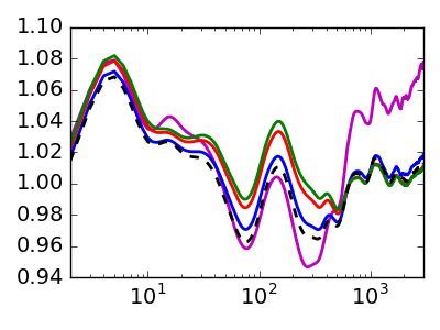
2
string loops that are produced throughout the evolution assumption does not have a significant impact on the fi-
of a cosmic string network in Sec. III B. We characterize nal results1 . Moreover, we will also assume that the loop
the CMB signatures generated by cosmic string loops in has a translational velocity, vl , orthogonal to the loop’s
Sec. IV A, study their impact on the anisotropies gener- plane. In this case, we have that
ated by cosmic string networks in Sec. IV B and investi-
gate the impact of a reduced intercommutation probabil- X = Xi + Rc x cos σ + Rc y sin σ + vl τ z , (6)
ity in Sec. IV C. We then conclude in Sec. V.
where σ = σ 1 ∈ [0, 2π], and Xi is the initial location of
the center-of-mass of the loop. Here, x, y and z are three
II. STRESS-ENERGY TENSOR FOR orthogonal unitary vectors defined as
CIRCULAR LOOPS
sin θ sin φ
In most situations of interest in cosmology, a cosmic x = − sin θ cos φ , (7)
string may be treated as an infinitely thin object that cos θ
sweeps 1 + 1-dimensional worldsheet in spacetime. This cos φ cos ψ − sin ψ sin φ cos θ
worldsheet may be represented by the 4-vector y = sin φ cos ψ + sin ψ cos φ cos θ , (8)
sin θ sin ψ
X µ = X µ σ0 , σ1 ,
(1)
− cos φ sin ψ − cos ψ sin φ cos θ
where σ 0 and σ 1 are variables that parameterize the z = − sin φ sin ψ + cos ψ cos φ cos θ , (9)
string worldsheet. In this case, cosmic string dynamics sin θ cos ψ
is described by the Nambu-Goto action
with 0 ≤ θ < π and 0 ≤ φ, ψ < 2π.
Z
√ The Fourier transform of the stress-energy tensor of
S = −µ0 −γd2 σ , (2) the cosmic string loop is then given by
Z 2π
where µ0 is the cosmic string tension — which, for
Θµν = µ eik·X Ẋ µ Ẋ ν − −1 X 0 µ X 0 ν dσ. (10)
Nambu-Goto strings, coincides with the mass per unit 0
length — and is related to the energy-scale of the string
forming phase transition. Here γ is the determinant of Assuming, without loss of generality, that k = kkz , with
the worldsheet metric γab = gµν X,aµ ν
X,b (with a, b = 0, 1), kz = {0, 0, 1}, we have that
and gµν is the background metric.
In a Friedmann-Lemaitre-Robertson-Walker (FLRW) X · k = kXi · kz + vl τ zz + RkA sin(σ + B) , (11)
background — with line element
where
ds2 = a(τ )2 dτ 2 − dx2 ,
(3) xz
A2 = x2z + yz2 , tan B = , (12)
yz
where a(τ ) is the cosmological scale factor and dτ = dt/a
is the conformal time and t is the physical time — it is and the subscript ‘z’ denotes the projection along the kz
convenient to chose the temporal-transverse gauge: direction. The real part of “00”-component of the stress-
energy tensor (10) may then be written as
σ 0 = τ, and Ẋ · X0 = 0 , (4)
Θ00 = M J0 (X ) cos ϕ0 , (13)
where X µ = (τ, X) and a dot or a prime denotes a deriva-
tive with respect to σ 0 or σ 1 respectively. In this case, where M = 2πµ0 Rc γv , ϕ0 = kXi · kz + vl kτ zz , X =
the stress-energy tensor (obtained by varying the action kRc A, γv = (1 − vl2 )−1/2 , and Jn (..) is a Bessel function
in Eq. (2) with respect to gµν ) may be expressed as of the first kind.
µ0
Z The spatial components of the stress-energy tensor are
T µν = √ Ẋ µ Ẋ ν − −1 X 0 µ X 0 ν δ (4) d2 σ , (5) given by
−g
Θij = Θ00 ×
where δ (4) = δ (4) (xη − X η (σ 0 , σ 1 )) is a Dirac delta func-
γ −2 i j (14)
tion and 2 = X02 /(1 − Ẋ2 ). vl2 z i z j − v x x I− + y i y j I+ + 2Ix(i y j) ,
Let us now consider the case of a circular (planar) cos- 2
mic string loop with conformal radius Rc . For simplicity,
we shall assume that the loop has, instantaneously, no
radial velocity (Ṙc ≈ 0). Although cosmic string loops
are quite generally expected to oscillate under the effect 1 See Appendix A for the stress-energy tensor of a loop with R˙c =
6
of their tension, we have verified numerically that this 0.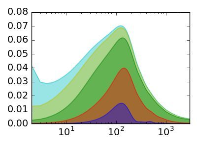
3

where                                                              where c̃ is a parameter that quantifies the loop-chopping
                                                                   efficiency, and k(v̄) is a momentum paremeter. Nambu-
              J2 (X )                    J2 (X )                   Goto simulations are well described by c̃ = 0.23 and a
  I± = 1 ±            cos 2B,          I=         sin 2B,
              J0 (X )                    J0 (X )                   momentum parameter of the form [25]
                                                            (15)
                                  1 i j                                            √
                     y (i xj)       y x + xi y j .                                2 2 1 − 8v̄ 6                  √

            and                 =
                                  2                                       k(v̄) =               (1 − v̄ 2 )(1 + 2 2v̄ 3 ), (19)
                                                                                    π 1 + v̄ 6
The scalar, vector and tensor components of the stress-            see Ref. [31] for the latest calibration of these parameters
energy tensor (14) are given, respectively, by                     from the simulation of Abelian-Higgs cosmic strings.
                                                                      Since the main objective of the present work is to study
                                                                   the potential impact of cosmic string loops on the CMB,
                  ΘS = 2Θ33 − Θ11 − Θ22 /2,

                                                                   we also need to describe the number (and length) of loops
                            ΘV = Θ13 ,                      (16)   produced throughout cosmic history. This subject has
                                T     12                           had considerable attention in the literature (see e.g. [32–
                            Θ =Θ ,                                 40]) since cosmic string loops are expected to give rise
                                                                   to a stochastic gravitational wave background that is ex-
while the trace Θ = Θii and velocity field ΘD = Θ03                pected to be within reach of gravitational wave experi-
are fixed by imposing local energy-momentum conserva-              ments in the near future. Here we shall adopt the semi-
tion [14].                                                         analytical approach of Ref. [37] since it allows for the
                                                                   characterization of the number of loops created through-
                                                                   out the realistic cosmological history (even through the
    III.     MODELING THE COSMIC STRING                            radiation-matter and matter-dark-energy transitions). In
              NETWORKS WITH LOOPS                                  this approach, it is implicitly assumed that the main
                                                                   energy-loss mechanism in a cosmic string network is the
  A cosmic string network has two primary constituents:            creation of loops. Thus, all the energy lost by the net-
long strings — cosmic strings that stretch beyond the              work (besides the loss that results from Hubble expan-
horizon — and subhorizon closed string loops. The cre-             sion) goes into the formation of loops. The characteristic
ation of loops happens persistently throughout the evo-            length of the network Lc may be regarded as a measure
lution of a cosmic string network due to string collisions.        of the energy density of the network
These loops detach from the long string network and                                                µ0
                                                                                             ρ= 2 2,                       (20)
evolve independently from it. Thus, there is a contin-                                            a Lc
ual energy loss by the long string network that plays a
                                                                   where ρ is the average energy density of the network.
crucial role in its dynamics. In this section, we review
                                                                   Thus, using Eq. (18), one finds that the energy density
the main aspects of cosmic string network dynamics and
                                                                   lost by the network is given by
loop production and extend the USM model to account
for cosmic string loops.                                                                   dρ                   v̄
                                                                                                        = c̃       ρ.            (21)
                                                                                           dt   loops          aLc
                                                                      In this approach, it is also generally assumed that cos-
   A.      Cosmic string network evolution and loop
                                                                   mic string loops are created with a length that is a fixed
                       production
                                                                   fraction of the characteristic length of the network at the
                                                                   time of creation
   The evolution of topological defect networks has been
extensively studied using numerical [19–23] and semi-                                        lcb = αLc (tb ) ,                   (22)
analytical [24–30] methods. The Velocity-dependent                 where 0 < α < 1 is a constant loop-size parameter and
One-Scale (VOS) model, in particular, provides a sim-              lcb is the comoving length of the cosmic string loop at
ple and yet informative description of the large-scale dy-         its time of birth tb . The loop-size parameter α may
namics of defect networks that grasps the main features            be calibrated using numerical simulations. Note, how-
of averaged network evolution. This model — initially in-          ever, that numerical simulations are not conclusive as to
troduced for cosmic strings [24, 25] but later generalized         the length of the loops produced in a cosmic string net-
to defects of arbitrary dimensionality [26–30] — provides          work’s evolution. Nambu-Goto simulations consistently
a quantitative description of the evolution of a long string       indicate that about 10% of the energy lost by the long
network by its root-mean-squared velocity (RMS) v̄ and             string network goes into the formation of large loops with
characteristic conformal length Lc [24]:                           α ∼ 0.34 [38, 41, 42]2 . Meanwhile, Abelian-Higgs simula-

                dv̄                 k(v̄)    ȧ
                    = (1 − v̄ 2 )         − 2 v̄ ,      (17)
                dτ                     Lc    a                     2   There is, however, a severe disagreement in the number of small
              dLc     ȧ            c̃                                 loops predicted by simulation-inferred models developed by dif-
                    = Lc v̄ 2 + v̄ ,                    (18)           ferent groups [43] (see, however, [42, 44]).
               dτ     a             2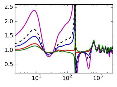
4
tions suggest much smaller density of loops due to an ad- where N (τi ) is the number of long string segments that
ditional mechanism of energy loss: the emission of scalar decay between τi−1 and τi , V is the simulation volume,
and gauge radiation [22, 45]. Here, we shall treat α as and n(τ ) is the number density of long strings
a free parameter of the model in order to study different
scenarios. The number density of loops created per unit C(τ )
n(τ ) = . (28)
time is then given by [37]: Lc (τ )3
Agreement between the number density of strings in this
dnl 1 dρ c̃ v̄
= b = . (23) model and that predicted by the VOS model is ensured by
dt alc dt loops α a4 L4c requiring that the normalization function C(τ ) is given
by V/Lc (τ )3 at any given conformal time τ .
Although, in reality, one does not expect all loops to
In order to include loops in this model, we assume that
be created with exactly the same length, the effect of
the segments that decay at a given time are “converted”
having a distribution of lengths at the moment of creation
into cosmic string loops and, thus, the number of loops
may, to some extent, be included in this model through
created at a given time is given by
a renormalization of Eq. (23) by a factor F [35, 38, 40].
After creation, cosmic string loops are expected to emit µ0 N (τi )Lc (τi ) N (τi )
gravitational radiation at a roughly constant rate Nl (τi ) = b
= , (29)
µ0 lc (τi ) α
dEl where we have used Eq. (22). This ensures that there is
= −ΓGµ20 , (24)
dt gr
a balance between the energy lost by the cosmic string
network and the total energy of the loops created, so
where Γ ∼ 50 [46, 47], that the number of loops created is in agreement with
Z Eq. (23).
El = µ0 a dσ = µ0 l (25) In this extension of the USM, the long string segments
decay at each (discrete) time instant τi and a population
of Nl (τi ) circular loops is created with an initial comoving
is the energy of the loop, and l = alc is the length of the
radius Rc (τi ) given by Eq. (26) and a stress-energy tensor
cosmic string loop. Loops then shrink as a result of this
given by Eqs. (13)-(14). These loops then shrink (by
emission until they eventually evaporate. In fact, using
emitting gravitational waves) according to Eq. (26) until
Eqs. (22)-(25), we find that the comoving radius of the
they eventually disappear at a time τf (in which Rc (τf ) =
cosmic string loop evolves as
0). The appearance/disappearance of the cosmic string
αLc (τi )a(τi ) − ΓGµ0 (t(τ ) − t(τi )) loops is achieved in the same manner as the decay of
Rc (τ ) = , (26) string segments in the original USM model. In fact, the
2πa(τ )
total stress-energy tensor of the loop network is written
where τi is the conformal time of birth of the loops and as
τf is the time of loop decay (for which Rc (τf ) = 0). NT
X
Θ̃µν
L (k, τ ) = Θµν
n (k, τ )T
off
(τ, τfn )T on (τ, τin ) , (30)
n
B. An Unconnected Segment Model with Loops
where Θµνn (k, τ ) is the stress-energy tensor of the n-th
loop, NT is the total number of loops, and τin and τfn are
This section extends the USM [13, 14] — which de-
respectively the conformal times of creation and evapo-
scribes the stress-energy tensor of a cosmic string net-
ration of the n-th loop. Here, we have also introduced
work — to also account for cosmic string loops. In the
the functions
USM, the long string network is modeled as a collection
of uncorrelated, straight finite segments created simulta- 1
τ < λ− τf
neously at an early time. The positions of the segments off
T (τ, τf ) = 21 + 14 x3off − 3xoff
λ− τf ≤ τ < τf ,
are drawn from a uniform distribution in space, and the
0 τf ≤ τ
direction of their velocities — which is assumed to be or-
thogonal to the string itself — is chosen from a uniform (31)
distribution on a two-sphere. The VOS model is then where
used to set the comoving length of the segments Lc and ln(λ− τf /τ )
the magnitude of their velocity v̄. Since our model also xoff = 2 − 1, (32)
ln(λ− )
includes the contribution of long strings (besides that of
loops), we preserve the main features of this model. and
To account for the energy loss caused by loops pro-
0
τ < τi
duction, a fraction of the segments decays at each time
T on (τ, τi ) = 1 1
+ 3xon − x3on τi ≤ τ < λ+ τi ,
instant τi : 2 4
1 λ+ τi ≤ τ
N (τi ) = V [n(τi−1 ) − n(τi )] , (27) (33)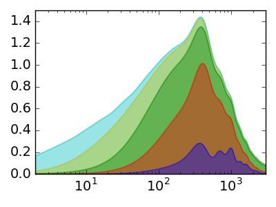
5

where                                                                     sum of their contributions to the stress-energy tensor in
                                                                          Fourier space corresponds to a sum of terms with ran-
                                 ln(τi /τ )
                      xon = 2               − 1.                 (34)     dom phases. Similarly to long strings, these may then be
                                ln(1/λ+ )                                 consolidated into a single loop located at the position of
                                                                          the center-of-mass of the decaying
                                                                                                        √      string at the time of
The T off function is responsible for “turning off” the con-
                                                                          creation τi , with a weight 1/ α. After this first consol-
tribution to the stress-energy tensor of loops that have
                                                                          idation step, we have N (τi ) loops that were created at
already evaporated at the time τf and it is identical to
                                                                          the same time τi and located at the (random) positions
the T off function used in the original USM to model the
                                                                          of the centers-of-mass of the decaying segments. We may
decay of long string segments. We have also included
                                                                          then consolidate   these loops into a unique loop with a
the T on function to “turn on” the contributions of all the                         p
                                                                          weight of N/α:
loops created at the time τi 3 . These functions then en-
sure that Θ̃µνLoops (k, τ ) only has a contribution from the                                Θ̃µν
                                                                                              L (k, τ ) =
relevant loop populations: those that were created at a                          q
                                                                               X                                                                    (35)
time τi < τ and have not evaporated completely yet at                        =    Nl (τij )Θµν
                                                                                            j (k, τ )T
                                                                                                       off
                                                                                                           (τ, τfj )T on (τ, τij ) ,
time τ . The constants λ± determine how fast loops ap-                            j
pear or disappear: in fact, T on (T off ) grows (decreases)
continuously from 0 (1) to 1 (0) between τi (λ− τf ) and                  where the index j runs over the consolidated loops.
λ+ τi (τf ). Here, we take λ± = 1 ± 0.24 .                                   The correlation between loops and long strings is taken
   An essential feature of the USM for long strings is that,              into account by positioning the consolidated loop — that
to ensure computational efficiency, all cosmic string seg-                represents the population of loops created at τi — at the
ments that decay at a given time are consolidated into a                  position of the consolidated decaying string segment at
single string segment. In fact, since the segments are dis-               the time of decay and by imposing that the direction of
tributed randomly in real space, their random positions                   the velocity of the loop coincides with that of the decay-
correspond to a random phase in Fourier space. Thus,                      ing string. We should then have
the amplitude of the sum of their contribution to the                                 ϕ0 = kX0 · kz + kτi zz v̄ + vl k(τ − τi )zz ,                 (36)
stress-energy tensor is essentially a 2-dimensional ran-
dom walk. As a result, the total stress-energy tensor in                  where X0 is the (randomly assigned) initial position of
Fourier space is simply the stress-energy√ tensor of a sin-               the decaying consolidated segment, X0 · kz + kτi zz v̄ is its
gle segment weighted by a factor of N [14]. Naturally,                    position at the time of decay. Since the center-of-mass
for numerical efficiency, we shall preserve this feature and              velocity of the loop is expected to scale as γv vl ∝ a−1
consolidate each loop population — i.e. the loops that                    due to the expansion of the background, the velocity of
are created (and decay) at the same time — into a single                  the loop is given by
cosmic string loop. However, cosmic string loops cannot
                                                                                                                  vl (τi )
realistically be expected to follow a random distribution                             vl (τ ) = r                                                   (37)
                                                                                                                                               2
in space. As a matter of fact, as discussed in Ref. [18],

                                                                                                                                      a(τ )
                                                                                                    vl2 (τi ) + (1 − vl2 (τi ))       a(τi )
the positions of loops are highly correlated with the posi-
tions of long strings: loops are created along the strings,
                                                                          at any instant of time τ > τi .
and they tend to move in the same direction as the string
from which they are chopped. Assuming that loops are
randomly distributed in space and move in random direc-                     IV.       COSMIC MICROWAVE BACKGROUND
tions is, therefore, not realistic and may have a significant                                ANISOTROPIES
impact on the results. However, in any case, we can con-
solidate a loop population into a single loop if we do so
                                                                             Although the CMB has a nearly perfect black body
in two steps. At any given time τi , N (τi ) segments de-
                                                                          spectrum with an approximately uniform temperature,
cay into loops, and thus, we have, on average, α−1 loops
                                                                          there are tiny temperature fluctuations across the sky [4].
created per decaying string segment. Given the strong
                                                                          The CMB is generally characterized in terms of the angu-
correlation between the positions of strings and loops,
                                                                          lar power spectrum, C` , of the temperature fluctuations
we may then expect that these α−1 loops are created at
random positions along the decaying string and thus the                                                     `
                                                                                                       1    X
                                                                                            C` =               ha∗ a`m i ,                          (38)
                                                                                                    2` + 1 m=−1 `m

3   The USM, in its original implementation [14], actually included,      where angled brackets represent an ensemble average.
    for computational efficiency, a slightly different T on function to   Here, a`m are the coefficients of the decomposition of the
    only “turn on” segments once they may contribute significantly        temperature fluctuations, 4(n̂) = 4T /T , into spherical
    to the CMB anisotropies. This was, however, abandoned in later        harmonics
    extensions of the model.
4
                                                                                                    X
    We have verified numerically that the values of λ± do not have                        4(n̂) =       a`m Y`m (n̂) ,          (39)
    a significant impact on the final results
                                                                                                            `m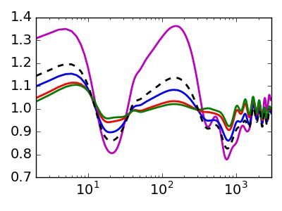
6

where n̂ is the direction of the line of sight and Y`m are
spherical harmonic functions. The angular power spec-                                   10 -1
trum, then, allows us to separate the contributions to
                                                                                        10 -2

                                                               ¤
different angular scales of the CMB anisotropies.

                                                                  4πP(k) (hMpc −1 ) 3
   Here, we are also going to compute the Cold Dark Mat-                                10 -3
ter (CDM) linear power spectrum,
                                                                                        10 -4

                                                               £
                               2
                    P (k) = δ (k) ,                   (40)
                                                                                        10 -5
where δ (k) is the Fourier transform of the density con-
                                                                                        10 -6
trast,
                                                                                        10 -7
                         ρm (x) − hρm i                                                         10 -3     10 -2   £       ¤
                                                                                                                                  10 -1
                 δ (x) =                ,             (41)                                                   k/h Mpc −1
                             hρm i

where ρm (x) is the matter density at a given position x
and hρm i is its average value.                               Figure 1. Linear CDM power spectrum generated by cosmic
   In this section, we compute the CMB and linear CDM         string loops. We include the CDM power spectra generated
                                                              by cosmic string loops up to a = 10−4 (blue line),a = 10−3
power spectra generated by cosmic string networks with
                                                              (red line), a = 10−2 (green line), a = 10−1 (olive line), and
loops. To do this, we extend the publicly available CM-       a = 1 (cyan line). We have averaged over 500 realizations
BACT code to also account for cosmic string loops, by         of cosmic string loop networks, and took Gµ0 = 10−7 and
implementing the modifications described in the previous      α = 10−1 .
sections. Our results are obtained by averaging over 500
realizations of a brownian cosmic string network with
the following cosmological parameters: Ω0b h2 = 0.0224,
Ω0m h2 = 0.1424 for baryon and matter density parame-         evolution decreases with time because the network be-
ters, and H0 = 100h kms−1 Mpc−1 , with h = 0.674 for the      comes progressively less dense. As a result, the dom-
Hubble parameter at the present time [48]. The tension        inant contribution to the CDM power spectrum comes
of cosmic strings is fixed to Gµ0 = 10−7 and we assume        from loops created in the radiation era or around the
that all loops are created with the same length (and thus     radiation-matter transition.
F = 1) unless stated otherwise. The unmodified CM-
BACT is used to obtain the power spectra generated by                                    10 0
long strings only.
                                                              ¤
                                                               4πP(k) (hMpc −1 ) 3

                                                                                        10 -1
    A.    The contribution of cosmic string loops
                                                                                        10 -2
   Before going into the CMB anisotropies generated by                                                                                    vl2 = 0
                                                              £

the full cosmic string network, with both long strings and
loops, we start by presenting the contribution that comes                               10 -3                                             vl2 = 0. 5
solely from cosmic string loops. To do so, we modify                                                                                      vl2 = 0. 999
the CMBACT code in such a way as to include only the                                    10 -4
contribution of cosmic string loops to the stress-energy                                          10 -3   10 -2   £           ¤
                                                                                                                                  10 -1
                                                                                                                      −1
tensor (35).                                                                                               k/h Mpc
   Let us start by looking into the linear CDM power
spectrum. To have a clear picture of the contribution
of cosmic string loops, we have studied the evolution of      Figure 2. Linear CDM power spectrum generated by cosmic
the linear CDM power spectrum generated by loops. In          string loops with different velocities. We chose Gµ0 = 10−7
particular, in Fig. 1, we plot the linear CDM power spec-     and α = 10−1 and averaged over 500 realizations of cosmic
trum generated by cosmic string loops up until different      string and/or loop network realizations.
epochs in cosmic history (namely until a scale factor of
a = 10−4 , a = 10−3 , a = 10−2 , a = 10−1 , and a = 1,
corresponding to the present time). Therein, we may see          In Fig. 2, we plot the linear power spectrum generated
that, as time progresses, cosmic string loops contribute      by randomly distributed cosmic string loops for differ-
dominantly at increasingly larger scales (smaller values      ent values of the loop translational velocity. Therein,
of k). As a matter of fact, since the correlation length of   one may see that for static loops the power spectrum is
the cosmic string network increases throughout the evo-       flat for sufficiently large k (or small scales) as predicted
lution, the radius of the loops produced also increases.      in [18]. This is mainly a result of the fact that static
However, the number of loops created throughout the           loops act, on sufficiently large scales, effectively as point-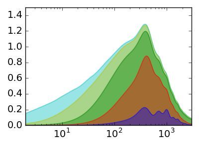
7
values of k.
10 0
As Fig. 3, where we plot the linear CDM power spec-
¤
4πP(k) (hMpc −1 ) 3
trum of loops alongside that of long strings, shows, ex-
10 -1 cept for the slower decrease at small scales, the spectrum
generated by cosmic string loops is very similar both in
10 -2 amplitude and in shape to that generated by long strings.
Both have peaked power spectra due to the enhancement
£
10 -3
long strings+loops of perturbations caused by the fact that there is a large
loops number of sources with approximately the same length
long strings at roughly the same distance; however, in the case of
10 -4 loops, the peak is located at larger k because the length
10 -3 10 -2 £ ¤
10 -1 of the loops is a fraction of the correlation length of
−1
k/h Mpc long strings. Moreover, since loops decay after forma-
tion, there is some dispersion in the length of the sources
of perturbation, and, as a result, the peak of the spec-
Figure 3. Linear CDM power spectrum generated by a cos- trum is broader and less pronounced.
mic string network with loops. The solid (blue) line represents The differences in the CDM linear power spectrum of
the power spectrum generated by cosmic strings and cosmic long strings and loops naturally translate into differences
string loops, while the dash-dotted (black) and dashed (red) in the CMB anisotropies. In Fig. 5 the TT, EE, TE and
lines represent the contributions of long strings and cosmic
BB components of the CMB angular power spectra gen-
string loops. We chose Gµ0 = 10−7 and α = 10−1 and aver-
aged over 500 realizations of cosmic string and/or loop net-
erated by cosmic string loops are plotted up to different
work realizations. cosmological scale factors. The shape of angular spectra
for cosmic loops is also very similar to that generated
by long string networks (cf. Fig. 7), but its maximum
amplitude is about one order of magnitude smaller, and
6 4. 48 × ` −0. 06 the peaks of the spectra also appear at a smaller angular
scale (or larger multipole `). The most noticeable differ-
¤
Total
µK 2
5 Scalar ence, however, appears in the vector components. As a
Vector matter of fact, the vector contribution to the temperature
£
4
CTT `(` + 1)/(2π)
Tensor anisotropies does not decrease with the increase of multi-
pole moment ` (decreasing angular scales) as it happens
3
for long strings. We anticipate that small circular loops
2 are responsible for this effect: due to their shape, they
actively generate rotational movements of matter, giving
1 rise to the divergenceless (vortical) velocity field. In par-
ticular, for ` > 1500, the vector contribution to the TT
0 angular power spectrum generated by loops is approxi-
0 500 1000 1500 2000 2500 3000
` mately constant, as shown in Fig. 4, while for long strings
CT T `(`+1)
2π ∼ `−1.5 [49].
Fig. 5 also shows that cosmic string loops generate tem-
Figure 4. Temperature angular power spectrum generated by perature anisotropies at progressively larger scales be-
cosmic string loops and its scalar, vector, tensor components. tween the epoch of the last scattering and the present
For ` > 1500 the total contribution is well approximated by
time since the length of loops (at the moment of cre-
CT T `(`+1) ∼ `−0.05 , i.e it is almost constant due to the vector
2π ation) increases with time. However, since the number
contribution.
of created loops decreases roughly as t−4 , the dominant
contribution (corresponding to the peak of the spectrum)
is generated earlier in cosmological history. The polariza-
like sources of perturbations. On the other hand, if the tion anisotropies — as is the case for long strings and do-
loops are moving, they generate filament-like perturba- main walls — are created mainly in two epochs: the dom-
tions, which causes a transfer of power towards larger inant peak at small angular scales is generated around the
scales (smaller k). Although this effect is more accen- last scattering (a ∼ 10−3 ), while the large-scale subdom-
tuated for larger value of vl , our results show that the inant peak is created around the epoch of reionization
amplitude and shape of the linear power spectrum does (a ∼ 10−1 ).
not depend strongly on the magnitude of the velocity The CMB power spectra generated by cosmic string
of loops. However, this figure also shows that, for non- loops with different translational velocities (vl2 = 0,
vanishing vl , the spectrum starts to develop a decreasing vl2 = 0.5, vl2 = 0.999) are plotted in Fig. 6. The results
slope at small scales, exhibiting signs of the transition show that, although the general shape of the spectrum
to the k −1 regime predicted in Ref. [18] for even larger does not depend significantly on the velocity of loops (see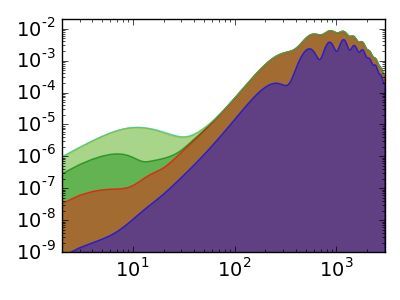
8
Fig.2), the amplitude of the anisotropies does. The tem- B. CMB anistropies generated by cosmic string
perature anisotropies, in particular, are highly dependent networks with loops
on the speed of loops and generally increase with increas-
ing vl . Vector and tensor modes, due to their nature, are In this section we will characterize the CMB
more affected, while scalar modes do not have such sig- anisotropies generated by a cosmic string network, in-
nificant change, as shown in Fig 6. Note however that, cluding both loops and long strings. To do so, we imple-
in general, we do not expect loops to be static or non- mented the extension of the USM described in Sec. III B
relativistic. In fact, they are expected to move with rela- in the CMBACT code. In particular, we write the to-
tivistic speeds and smaller loops to have higher velocities tal stress-energy tensor of the network as a sum of the
in general. Here and through the remainder of this pa- contributions of loops and long strings,
per, we shall take vl2 = 0.5 unless stated otherwise. Since
the contribution of loops is expected to be subdominant Θµν µν µν
Network (k, τ ) = ΘS (k, τ ) + Θ̃L (k, τ ) , (42)
when compared to that of long strings, this assumption
is not expected to have a significant impact on the final where ΘµνS (k, τ ) is the stress-energy tensor of long strings
results. as described in the original USM [13, 14] (which includes
the contribution of all consolidated string segments) and
Θ̃µν
L (k, τ ) is given by Eq. (30). As discussed in the previ-
ous section, numerical simulations show a strong correla-
tion between the positions and velocities of long strings
and cosmic string loops [18]. This vital ingredient is
taken into account in this computation by imposing that
the loops are created where a consolidated long string
has decayed. Moreover, the loop velocity vl is orientated
along the same direction as the long string velocity v̄, as
it is encoded in Eq. (36).
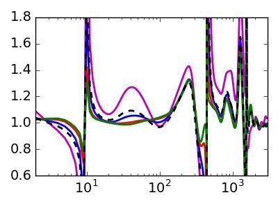
Figure 5. CMB anisotropies generated by cosmic string loops. From left to right, we plot the TT,TE, EE and BB power
spectra, as a function of the multipole moment `. The top, middle and bottom rows represent the scalar,vector and tensor
components, respectively. In each of the plots we include the angular power spectra generated by cosmic string loops until
a = 10−4 (blue line), a = 10−3 (red line), a = 10−2 (green line), a = 10−1 (olive line), and a = 1 (cyan line). We have averaged
over 500 realizations of cosmic string loop networks, and took Gµ0 = 10−7 , α = 10−1 .
The CDM linear power spectrum generated by cosmic string networks with loops is plotted in Fig. 3, along-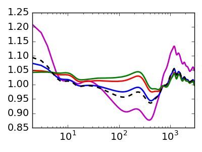
9

Figure 6. CMB anisotropies generated by cosmic string loops with different velocities. From left to right, we plot the TT,
TE, EE and BB power spectra, as a function of the multipole moment `. The top, middle and bottom rows represent the
scalar, vector and tensor components, respectively. Each of the plots represents different values of translation velocities vl2 = 0
(dash-dotted red line), vl2 = 0.5 (dashed blue line), vl2 = 0.999 (solid green line), while Gµ = 10−7 , α = 10−1 and the results
are obtained by averaging over 500 realizations.

Figure 7. CMB anisotropies generated by cosmic string networks with loops. From left to right, we plot the TT, TE, EE and
BB power spectra, as a function of the multipole moment `. The top, middle and bottom rows represent the scalar,vector and
tensor components, respectively. In each panel, we include the CMB anisotropies generated by a cosmic string network with
loops (solid blue line), as well as the contribution of long strings (dash-dotted black line) and cosmic string loops (dashed red
line). The result is obtained by averaging over 500 realizations of cosmic string networks.

side that of cosmic strings and that of (randomly dis-             tributed) loops. Therein one may see that, as a result of
10
BOS
Figure 8. Ratio between the CMB anisotropies generated by cosmic string networks with loops, C`S+l , and those generated by
long strings only, C`S , for different loop sizes. From left to right, we plot the TT, TE, EE and BB power spectra, as a function
of the multipole moment `. The top, middle and bottom rows represent the scalar, vector and tensor components, respectively.
Each panel includes the anisotropies generated by networks with α = 10−1 , α = 10−2 , α = 10−3 , α = 10−4 and for the loop
distribution inferred from the simulations of Blanco-Pillado, Olum and Shlaer (BOS) in Ref. [38].
8 but its maximum amplitude increases by a factor of 2−3.
α = 10 −1
7 α = 10 −2 The CMB anisotropies generated by a cosmic string
6 α = 10 −3 network with loops (in both the temperature and polar-
P S + l (k)/P S (k)
5 α = 10 −4 ization channels) are plotted in Fig. 7. In these plots,
BOS we may see that loops with α = 10−1 roughly contribute
4 to about 10% of the anisotropies and lead to a visible
3 increase for large multipole moments `. This enhance-
2 ment is particularly significant in the vector modes —
1 since, as discussed before, loops generate (due to their
shape) vortical motions of matter — and, in the case of
0
10 -3 10 -2 10 -1 the TT vector anisotropies, there is a significant increase
k/h Mpc −1 for l & 1000. Current Planck constraints on Nambu-Goto
strings [50] — which limit their fractional contribution to
temperature anisotropies to about 1−2% — were derived
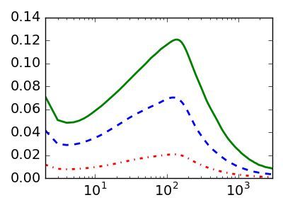
Figure 9. Ratio between the linear CDM power spectrum gen-
using the original USM model and thus do not include
erated by cosmic string networks with loops, P S+l (k), and the effect of loops. Our results then indicate that the in-
that of long strings, P S (k), for different loop sizes. We in- clusion of loops may result in more stringent constraints
clude the CDM power spectra generated by networks with on cosmic string tension. Note also that, although the
α = 10−1 , α = 10−2 , α = 10−3 , α = 10−4 and for the BOS shape of the power spectra generated by cosmic string
distribution. networks with loops is very similar to that of long strings,
the contribution of loops to the vector-mode temperature
anisotropies is dominant for large multipole moments `.
As a result, the temperature anisotropies decrease more
the correlations, the effect of including loops is to enhance slowly with increasing ` if loops are included. This is in
the spectrum of perturbations generated by strings. The agreement with the results of Ref. [10] — derived using
shape of the power spectrum is not significantly affected numerical simulations that include loops — in which the
— except on small scales wherein the decrease is some- TT anisotropies scale as `−0.89 for large angular scales
what slighter than k −2 due to the inclusion of loops — (whereas, for the USM model, the TT angular power11 spectrum behaves asymptotically as `−1.5 [49]). Our re- as we lower cosmic string tension. As a matter of fact, the sults indicate that this discrepancy may indeed be related amplitude of CMB anisotropies generated by loops scales to the contribution of cosmic string loops. as C` ∝ (Gµ0 )2 (as does that of long strings) and thus the The impact of the inclusion of loops on the anisotropies shapes of the (total) angular power spectra are roughly is highly dependent on the size of loops. Figs. 8 and 9 maintained. Note also that, in our computations of the — where we plot the TT, TE, EE and BB anisotropies CMB generated by cosmic string networks with loops, we and the linear CDM power spectrum generated by cosmic have assumed that F = 1 (except for the spectra gener- string networks with loops of different sizes (normalized ated by Nambu-Goto cosmic string networks with loops). to that of long strings) — clearly show this effect. There If we relax the assumption that all loops are created with we also include the spectra generated by Nambu-Goto the same size and assume thus that F 6= 1, the amplitude cosmic string networks with loops calibrated by the latest of the CMB anisotropies would be suppressed by a factor simulations in Ref. [38]. This is done by setting α ≈ of F 1/2 . The specific value of F, however, would depend 0.34, vl = 0.42, and by correcting the number of loops on the particular distribution assumed for the length of produced by a factor of F = 0.1 (to account for the produced loops. If the width of the distribution is not fact that only about 10% of the energy lost by network very large, we do not expect this assumption to affect goes into the formation of loops). Our results indicate the results significantly, but if there is a large spread this that, for this scenario, the impact of cosmic string loops may have an impact on the final results. on small scales is still significant. Loops then should be considered in the derivation of observational constraints on the tension of Nambu-Goto strings. C. Strings with reduced intercommutation Our results show that the contribution of loops remains probability relevant as the length of the loop decreases. Note how- ever that the correlation between the positions and ve- Until now, we have assumed that the intercommuta- locities of long strings and loops play a determinant role tion probability P is equal to 1 and thus that whenever here: for randomly distributed loops (as the ones consid- cosmic strings collide they exchange partners and recon- ered in the previous section) the CMB anisotropies die nect. However, several brane-inflationary scenarios [51– off quickly with decreasing α (roughly C` ∝ α). How- 53] predict the production of fundamental strings (or ever, since loops are distributed along the strings, these F-strings) and one-dimensional D-branes (or D-strings) loops, even if small, enhance the perturbations that have that may grow to macroscopic sizes and play the cos- been generated by the long strings. In fact, as the size mological role of cosmic strings [54–56]. These cosmic of loops decreases, there are two competing effects: the superstrings may, unlike ordinary strings, have an in- number of loops increases (as Nl ∝ α−1 ); but these loops tercommutation probability that is significantly reduced are smaller and survive for a shorter period of time. The due to their quantum nature [57–59] and/or the exis- net result is that, as these figures show, a decrease of tence of extra dimensions [60]. In this section, we in- the loops’ length leads to a decrease of the impact of vestigate whether the contribution of cosmic string loops loops on both the spectrum of perturbations and CMB to the CMB anisotropies remains significant for string anisotropies. The excess in the vector modes in the tem- networks with a reduced intercommutation probability. perature anisotropies quickly decreases with decreasing α Note however that, although cosmic superstrings serve and, as a result, the constraints on scenarios with smaller as the motivation for this study, there are several impor- loops are necessarily less stringent. Interestingly, how- tant properties of these networks that will not be taken ever, there is an excess in tensor modes even for small into consideration. In particular, since F- and D-strings α, especially in the polarization channels: tensor modes do not intercommute, but instead bind together to cre- actually increase as α decreases for 10 . ` . 103 . We ate a new (heavier) type of string, their collision leads have verified numerically that this trend continues if we to the production of Y-type junctions. Moreover, subse- decrease α further, even beyond the gravitational back- quent collisions are expected to give rise to even heavier reaction scale (ΓGµ0 ), but the decrease in temperature (p, q)-strings — composed of q F-strings and p D-strings anisotropies and the increase in polarization anisotropies — and thus cosmic superstrings are expected to form en- is significantly slower. In fact, there seems to be a resid- tangled multi-tensional networks (see e.g Refs. [61–64]). ual excess (similar in magnitude to that observed for The heavier string types and junctions may have a sig- α = 10−4 ) in both the temperature and polarization nificant impact on the network’s dynamics [60, 62] and channels as a result of the inclusion of loops, even if they observational signatures [63, 65]. The work in this sec- are quite small. The B-mode polarization channel may tion should, then, be regarded as exploratory, but our then offer us an alternative window to probe the size of results may indicate us whether it is worth performing a cosmic string loops. more profund study. Note that, although here we only plotted the CMB When two strings with reduced intercommutation anisotropies generated by cosmic string networks with probability collide, there is a 1 − P probability that they loops for Gµ0 = 10−7 , we have verified that the contri- merely pass through each other without interaction. This bution of loops to the CMB anisotropies remains relevant naturally results in a decrease of the loop-chopping effi-
12

                                               Scalar+Vector+Tensor modes
                                                                                               where c̃(1) = 0.23 is the loop-chopping efficiency of net-
                                                                                               works with P = 15 . These networks are, then, weakly
                                                                                               interacting and consequently significantly denser, with a
                                                                                               characteristic length of aLc ∼ P 1/3 and ρ ∝ P −2/3 [68].
                                                                                               As a result, the energy density lost due to loop formation
                                                                                               is actually enhanced as P is reduced:
                                                                                                                       dρ
                                                                                                                                    ∝ P −2/3 .              (44)
                                                                                                                       dt   loops

                                                                                               Note however that, although the number of loops created
                                                                                               (per unit volume) increases as P decreases, the length of
                                                                                               the loops is expected to decrease since the characteristic
                                                                                               length of these networks is smaller. The combination of
                                                                                               these two effects actually results in a decrease of the con-
                                                                                               tribution of loops to the anisotropies and perturbation
                                                                                               spectra. This is illustrated in Figs. 10 and 11, where the
                                                                                               CMB and CDM power spectra generated by cosmic string
                P=5·10-1                  P=10-1           P=5·10-2        P=10-2   P=5·10-3   networks with loops for different values of the intercom-
                                                                                               mutation probability are plotted (normalized to those of
Figure 10. Ratio between the CMB anisotropies generated by                                     long strings). Note however that, although the amplitude
cosmic string networks with loops, C`S+l , and those generated                                 of the contribution clearly decreases with decreasing P ,
by long strings, C`S , for different intercommutation probabil-                                the contribution of loops at small angular scales (large `)
ities and α = 10−1 . We plot the total TT, TE, EE and BB                                       remains significant both in the temperature and polar-
angular power spectra, as a function of the multipole moment                                   ization channels. Our results indicate that the inclusion
`. Each panel includes the CMB anisotropies for P = 5 · 10−1 ,
                                                                                               of loops in computations of the CMB anisotropies gen-
P = 10−1 , P = 5 · 10−2 , P = 10−2 , P = 5 · 10−3 .
                                                                                               erated by cosmic superstring networks may be necessary
                                                                                               to obtain more accurate results. In fact, this contribu-
                                                                                               tion may be particularly relevant for the lightest strings
                       6                                                                       (the F-strings), which have a higher intercommutation
                                   P = 5 · 10 −1                                               probability when compared to heavier string types.
                       5           P = 10 −1
                                   P = 5 · 10 −2
 P S + l (k)/P S (k)

                                   P = 10 −2
                       4           P = 5 · 10 −3                                                        V.   CONCLUSIONS AND OUTLOOK

                       3                                                                          In this paper, we have studied the impact of loops on
                                                                                               the cosmic microwave anisotropies generated by cosmic
                       2                                                                       string networks. To do so, we have extended the USM
                                                                                               — which describes the stress-energy tensor of a network
                       1                                                                       of long strings — to also account for the contribution
                           10 -3                   10 -2                   10 -1               of loops and implemented this extended version on the
                                                     k/h Mpc −1                                publicly available CMBACT code.
                                                                                                  Our results show that cosmic string loops may signifi-
                                                                                               cantly contribute to the CMB anisotropies on small an-
Figure 11. Ratio between the linear CDM power spectrum                                         gular scales (or large multipole moments) on both the
generated by cosmic string networks with loops, P S+l (k),                                     temperature and polarization channels. This may lead
and that generated by long strings, P S (k), for different in-
                                                                                               to more stringent CMB constraints on cosmic string ten-
tercommutation probabilities and α = 10−1 . We include the
spectra generated by networks with P = 5 · 10−1 , P = 10−1 ,                                   sion for scenarios with larger loop lengths. We further
P = 5 · 10−2 , P = 10−2 , P = 5 · 10−3 .                                                       demonstrated that loops with different sizes generate dis-
                                                                                               tinct signatures on the polarization angular power spec-
                                                                                               tra. As a result, B-mode polarization may be used to
                                                                                               probe different loop-formation scenarios.
ciency and, consequently, of the network’s energy losses.                                         Since loops are expected to decay by emitting gravita-
As a matter of fact, radiation and matter era numerical                                        tional radiation and to give rise to a stochastic gravita-
simulations of cosmic string networks in Ref. [66] with                                        tional wave background, loop-forming scenarios may also
P < 1 indicate that

                                                                                               5   Note however that Minkowski space simulations seem to indicate
                                              c̃(P ) = c̃(1)P    1/3
                                                                       ,               (43)        that c̃ ∝ P 1/2 instead [67].
13
be probed independently using gravitational wave exper- in fact, expected to stabilize after reaching a critical ra-
iments. Current pulsar-timing data set an upper limit for dius and survive throughout cosmological history [74, 75].
the tension of cosmic strings of about Gµ0 . 10−11 for These stable superconducting loops, known as vortons,
large loops [69, 70] and Nambu-Goto strings [71], which have been proposed as possible dark-matter candidates
is beyond the reach of CMB experiments. Note however and may lead to specific CMB signatures [76]. Note, how-
that pulsar-timing constraints on scenarios with smaller ever, that current is expected to have a significant impact
loops are 3 to 4 orders of magnitude weaker [69, 70] and on cosmic string dynamics [77] and axion string loops are
thus the CMB anisotropies may be a competitive inde- also expected to lose energy at a slower rate. The com-
pendent probe of these scenarios. putation of the signatures of vortons on the CMB would
then require an extension of this framework to account
Although we have mostly considered standard cos-
for these properties.
mic string networks in this paper, this framework may
be extended to study more exotic scenarios. Here, we
have investigated networks with reduced intercommuta- ACKNOWLEDGMENTS
tion probability as a proxy for cosmic superstring net-
works. Our results indicate that loops may provide a sig-
The authors thank Pedro P. Avelino for many fruit-
nificant contribution in the case of cosmic superstrings
ful discussions. L. S. is supported by Fundação para
too. Note however that a more detailed study, includ-
a Ciência e a Tecnologia (FCT) through contract No.
ing the contributions of different types of strings and
DL 57/2016/CP1364/CT0001. Funding of this work
junctions, would be necessary before these results can
has also been provided by FCT through national funds
be safely extrapolated to cosmic superstrings.
(PTDC/FIS-PAR/31938/2017) and by FEDER—Fundo
This framework may also be helpful to study the CMB Europeu de Desenvolvimento Regional through COM-
signatures of vortons. Axion strings are superconducting PETE2020 - Programa Operacional Competitividade
and give rise to loops that carry a current [72, 73]. After e Internacionalização (POCI-01-0145-FEDER-031938),
creation, these loops decay radiatively, but their current and through the research grants UID/FIS/04434/2019,
prevents them from evaporating completely. They are, UIDB/04434/2020 and UIDP/04434/2020.
Appendix A: Stress-energy for loops with Ṙc 6= 0
It is also possible to obtain a more general expression for loops with Ṙc 6= 0. In this case, we have
X = X0 + R(γv−1 τ )x cos σ + R(γv−1 τ )y sin σ + vτ z . (A1)
Substituting (A1) in the stress-energy tensor (10), we obtain
Θ00 = M γR J0 (X ) cos ϕ0 , (A2)
where γR = (1 − Ṙ2 )−1/2 and
xi xj 2 yi yj x(i y j)
−2 −2
Θij = Θ00 v 2 z i z j + Ṙ I+ − γ R I− + Ṙ 2
I − − γ R I + − I −
2γv2 2γv2 γv2 (A3)
v h (i j) i
−2M γR Ṙ x z sin B + y (i z j) cos B J1 (X ) sin ϕ0 ,
γv14
The scalar, vector and tensor contribution from the stress energy tensor (10) can be expressed as
Θ00 2 3 3 γ −2 3 3
ΘS = v (3z z − 1) + v (3x x − 1)(−1 + 2Ṙ2 + Y ) + (3y 3 y 3 − 1)(−1 + 2Ṙ2 − Y ) − 6Ix3 y 3 −
2 2
v h (i j) i
−2M γR Ṙ x z sin B + y (i z j) cos B J1 (X ) sin ϕ0 ,
γv
−2
γ
ΘV = Θ00 v 2 z 1 z 3 + v x1 x3 (−1 + 2Ṙ2 + Y ) + y 1 y 3 (−1 + 2Ṙ2 − Y ) − I(x1 y 3 + x3 y 1 ) −
2 (A4)
v 1 3
(x z + x3 z 1 ) sin B + (y 1 z 3 + y 3 z 1 ) cos B J1 (X ) sin ϕ0 ,
−M γR Ṙ
γv
−2
γ
ΘT = Θ00 v 2 z 1 z 2 + v x1 x2 (−1 + 2Ṙ2 + Y ) + y 1 y 2 (−1 + 2Ṙ2 − Y ) − I(x1 y 2 + x2 y 1 ) −
2
v 1 2
(x z + x2 z 1 ) sin B + (y 1 z 2 + y 2 z 1 ) cos B J1 (X ) sin ϕ0 .
−M γR Ṙ
γv
[1] M. B. Hindmarsh and T. W. B. Kibble, Cosmic Rev. D 33, 2182 (1986).
strings, Rept.Prog.Phys. 58, 477 (1995), arXiv:hep- [12] J. Traschen, N. Turok, and R. Brandenberger, Microwave
ph/9411342v1 [astro-ph.CO]. anisotropies from cosmic strings, Phys. Rev. D 34, 919
[2] A. Vilenkin and E. P. S. Shellard, Cosmic Strings and (1986).
Other Topological Defects (Cambridge University Press, [13] L. Pogosian and T. Vachaspati, Cosmic microwave back-
Cambridge, 2000). ground anisotropy from wiggly strings, Phys.Rev. D60,
[3] E. J. Copeland and T. W. B. Kibble, Cosmic strings 083504 (1999), arXiv:astro-ph/9903361v4 [astro-ph.CO].
and superstrings, Proceedings of the Royal Society A: [14] A. Albrecht, R. A. Battye, and J. Robinson, Detailed
Mathematical, Physical and Engineering Sciences 466, study of defect models for cosmic structure forma-
623 (2010), arXiv:0911.1345v3 [astro-ph.CO]. tion, Phys. Rev. D 59, 023508 (1998), arXiv:astro-
[4] D. J. Fixsen, E. S. Cheng, J. M. Gales, J. C. Mather, ph/9711121v2 [astro-ph].
R. A. Shafer, and E. L. Wright, The Cosmic Mi- [15] I. Yu. Rybak, A. Avgoustidis, and C. J. A. P. Mar-
crowave Background spectrum from the full COBE FI- tins, Semianalytic calculation of cosmic microwave
RAS data set, Astrophys. J. 473, 576 (1996), arXiv:astro- background anisotropies from wiggly and supercon-
ph/9605054. ducting cosmic strings, Phys. Rev. D96, 103535
[5] Planck Collaboration XXV (Planck), Planck 2013 re- (2017), [Erratum: Phys. Rev.D100,no.4,049901(2019)],
sults. XXV. Searches for cosmic strings and other topo- arXiv:1709.01839 [astro-ph.CO].
logical defects, Astron. Astrophys. 571, A25 (2014), [16] L. Sousa and P. P. Avelino, Cosmic microwave back-
arXiv:arXiv:1303.5085v1 [astro-ph.CO]. ground anisotropies generated by domain wall networks,
[6] J. Lizarraga, J. Urrestilla, D. Daverio, M. Hind- Phys. Rev. D 92, 083520 (2015), arXiv:1507.01064v1
marsh, and M. Kunz, New CMB constraints for [astro-ph.CO].
Abelian Higgs cosmic strings, JCAP 1610 (10), 042, [17] A. Avgoustidis, E. J. Copeland, A. Moss, and D. Skliros,
arXiv:1609.03386v3 [astro-ph.CO]. Fast analytic computation of cosmic string power spec-
[7] A. Lazanu, E. P. S. Shellard, and M. Landriau, Cmb tra, Phys. Rev. D 86, 123513 (2012), arXiv:1209.2461v2
power spectrum of nambu-goto cosmic strings, Phys. [astro-ph.CO].
Rev. D 91, 083519 (2015), arXiv:1410.4860 [astro- [18] J. H. P. Wu, P. P. Avelino, E. P. S. Shellard, and
ph.CO]. B. Allen, Cosmic strings, loops, and linear growth of mat-
[8] A. Lazanu and E. P. S. Shellard, Constraints on the ter perturbations, Int. J. Mod. Phys. D 11, 61 (2002),
nambu-goto cosmic string contribution to the cmb power arXiv:astro-ph/9812156.
spectrum in light of new temperature and polarisation [19] J. N. Moore, E. P. S. Shellard, and C. J. A. P. Martins,
data, JCAP 2015 (02), 024, arXiv:1410.5046v3 [astro- Evolution of abelian-higgs string networks, Phys. Rev. D
ph.CO]. 65, 023503 (2001), arXiv:hep-ph/0107171 [hep-ph].
[9] T. Charnock, A. Avgoustidis, E. J. Copeland, [20] C. J. A. P. Martins and E. P. S. Shellard, Fractal proper-
and A. Moss, Cmb constraints on cosmic strings ties and small-scale structure of cosmic string networks,
and superstrings, Phys. Rev. D 93, 123503 (2016), Phys. Rev. D 73, 043515 (2006), arXiv:astro-ph/0511792
arXiv:1603.01275 [astro-ph.CO]. [astro-ph].
[10] A. A. Fraisse, C. Ringeval, D. N. Spergel, and F. m. c. R. [21] J. J. Blanco-Pillado, K. D. Olum, and B. Shlaer,
Bouchet, Small-angle cmb temperature anisotropies in- Large parallel cosmic string simulations: New results
duced by cosmic strings, Phys. Rev. D 78, 043535 (2008), on loop production, Phys. Rev. D 83, 083514 (2011),
arXiv:0708.1162 [astro-ph]. arXiv:1101.5173 [astro-ph.CO].
[11] R. H. Brandenberger and N. Turok, Fluctuations from [22] M. Hindmarsh, J. Lizarraga, J. Urrestilla, D. Daverio,
cosmic strings and the microwave background, Phys. and M. Kunz, Scaling from gauge and scalar radiation inYou can also read