Neural network models and deep learning - a primer for biologists - arXiv
←
→
Page content transcription
If your browser does not render page correctly, please read the page content below
Neural network models and deep learning
– a primer for biologists
Nikolaus Kriegeskorte1,2,3,4 and Tal Golan4
1Department  of Psychology, 2Department of Neuroscience
3Department  of Electrical Engineering
4Zuckerman Mind Brain Behavior Institute, Columbia University

n.kriegeskorte@columbia.edu, tal.golan@columbia.edu

Originally inspired by neurobiology, deep neural network models have become a
powerful tool of machine learning and artificial intelligence. They can approximate
functions and dynamics by learning from examples. Here we give a brief
introduction to neural network models and deep learning for biologists. We
introduce feedforward and recurrent networks and explain the expressive power of
this modeling framework and the backpropagation algorithm for setting the
parameters. Finally, we consider how deep neural network models might help us
understand brain computation.

Neural network models of brain function
Brain function can be modeled at many different levels of abstraction. At one extreme,
neuroscientists model single neurons and their dynamics in great biological detail. At the
other extreme, cognitive scientists model brain information processing with algorithms
that make no reference to biological components. In between these extremes lies a model
class that has come to be called artificial neural network (Rumelhart et al., 1987; LeCun
et al., 2015; Schmidhuber, 2015; Goodfellow et al., 2016).
A biological neuron receives multiple signals through the synapses contacting its
dendrites and sends a single stream of action potentials out through its axon. The
conversion of a complex pattern of inputs into a simple decision (to spike or not to spike)
suggested to early theorists that each neuron performs an elementary cognitive function:
it reduces complexity by categorizing its input patterns (McCulloch and Pitts, 1943;
Rosenblatt, 1958). Inspired by this intuition, artificial neural network models are
composed of units that combine multiple inputs and produce a single output.
The most common type of unit computes a weighted sum of the inputs and transforms
the result nonlinearly. The weighted sum can be interpreted as comparing the pattern of
inputs to a reference pattern of weights, with the weights corresponding to the strengths
of the incoming connections. The weighted sum is called the preactivation. The strength
of the preactivation reflects the overall strength of the inputs and, more importantly, the
match between the input pattern and the weight pattern. For a given input strength
(measured as the sum of squared intensities), the preactivation will be maximal if the input
pattern exactly matches the weight pattern (up to a scaling factor).
Kriegeskorte & Golan (2019) Neural network models and deep learning

The preactivation forms the input to the unit’s nonlinear activation function. The activation
function can be a threshold function (0 for negative, 1 for positive preactivations),
indicating whether the match is sufficiently close for the unit to respond (Rosenblatt,
1958). More typically, the activation function is a monotonically increasing function, such
as the logistic function (Figure 1) or a rectifying nonlinearity, which outputs the
preactivation if it is positive and zero otherwise. These latter activation functions have
non-zero derivatives (at least over the positive range of preactivations). As we will see
below, non-zero derivatives make it easier to optimize the weights of a network.
The weights can be positive or negative. Inhibition, thus, need not be relayed through a
separate set of inhibitory units, and neural network models typically do not respect Dale’s
law (which states that a neuron performs the same chemical action at all of its synaptic
connections to other neurons, regardless of the identity of the target cell). In addition to
the weights of the incoming connections, each unit has a bias parameter: the bias is
added to the preactivation, enabling the unit to shift its nonlinear activation function
horizontally, for example moving the threshold to the left or right. The bias can be
understood as a weight for an imaginary additional input that is constantly 1.

Figure 1 | Function approximation by a feedforward neural network. A feedforward neural
network with two input units (bottom), three hidden units (middle), and two output units (top). The
input patterns form a two-dimensional space. The hidden and output units here use a sigmoid
(logistic) activation function. Surface plots on the left show the activation of each unit as a function
of the input pattern (horizontal plane spanned by inputs x1 and x2). For the output units, the
preactivations are shown below the output activations. For each unit, the weights (arrow
thickness) and signs (black, positive; red, negative) of the incoming connections control the
orientation and slope of the activation function. The output units combine the nonlinear ramps
computed by the hidden units. Given enough hidden units, a network of this type can approximate
any continuous function to arbitrary precision.
                                                                                                      2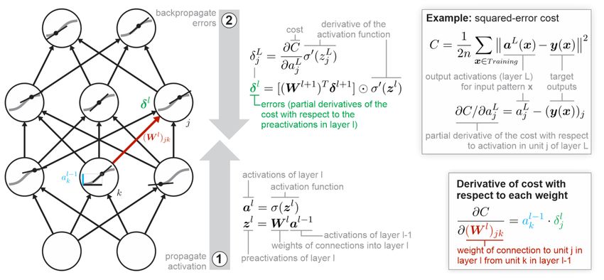
Kriegeskorte & Golan (2019) Neural network models and deep learning

Neural networks are universal approximators
Units can be assembled into networks in many different configurations. A single unit can
serve as a linear discriminant of its input patterns. A set of units connected to the same
set of inputs can detect multiple classes, with each unit implementing a different linear
discriminant. For a network to discriminate classes that are not linearly separable in the
input signals, we need an intermediate layer between input and output units, called a
hidden layer (Figure 1).
If the units were linear — outputting the weighted sum directly, without passing it through
a nonlinear activation function — then the output units reading out the hidden units would
compute weighted sums of weighted sums and would, thus, themselves be limited to
weighted sums of the inputs. With nonlinear activation functions, a hidden layer makes
the network more expressive, enabling it to approximate nonlinear functions of the input,
as illustrated in Figure 1.
A feedforward network with a single hidden layer (Figure 1) is a flexible approximator of
functions that link the inputs to the desired outputs. Typically, each hidden unit computes
a nonlinear ramp, for example sigmoid or rectified linear, over the input space. The ramp
rises in the direction in input space that is defined by the vector of incoming weights. By
adjusting the weights, we can rotate the ramp in the desired direction. By scaling the
weights vector, we can squeeze or stretch the ramp to make it rise more or less steeply.
By adjusting the bias, we can shift the ramp forward or backward. Each hidden unit can
be independently adjusted in this way.
One level up, in the output layer, we can linearly combine the outputs of the hidden units.
As shown in Figure 1, a weighted sum of several nonlinear ramps produces a qualitatively
different continuous function over the input space. This is how a hidden layer of linear–
nonlinear units enables the approximation of functions very different in shape from the
nonlinear activation function that provides the building blocks.
It turns out that we can approximate any continuous function to any desired level of
precision by allowing a sufficient number of units in a single hidden layer (Cybenko, 1989;
Hornik et al., 1989). To gain an intuition of why this is possible, consider the left output
unit (y1) of the network in Figure 1. By combining ramps overlapping in a single region of
the input space, this unit effectively selects a single compact patch. We could tile the
entire input space with sets of hidden units that select different patches in this way. In the
output layer, we could then map each patch to any desired output value. As we move
from one input region to another, the network would smoothly transition between the
different output values. The precision of such an approximation can always be increased
by using more hidden units to tile the input space more finely.

Deep networks can efficiently capture complex functions
A feedforward neural network is called ‘deep’ when it has more than one hidden layer.
The term is also used in a graded sense, in which the depth denotes the number of layers.
We have seen above that even shallow neural networks, with a single hidden layer, are
universal function approximators. What, then, is the advantage of deep neural networks?
Deep neural networks can re-use the features computed in a given hidden layer in higher
hidden layers. This enables a deep neural network to exploit compositional structure in a
                                                                                            3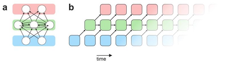
Kriegeskorte & Golan (2019) Neural network models and deep learning

function, and to approximate many natural functions with fewer weights and units (Lin et
al., 2017; Rolnick and Tegmark, 2017). Whereas a shallow neural network must piece
together the function it approximates, like a lookup table (although the pieces overlap and
sum), a deep neural network can benefit from its hierarchical structure. A deeper
architecture can increase the precision with which a function can be approximated on a
fixed budget of parameters and can improve the generalization after learning to new
examples.
Deep learning refers to the automatic determination of parameters deep in a network on
the basis of experience (data). Neural networks with multiple hidden layers are an old
idea and were a popular topic in engineering and cognitive science in the 1980s
(Rumelhart et al., 1987). Although the advantages of deep architectures were understood
in theory, the method did not realize its potential in practice, mainly because of insufficient
computing power and data for learning. Shallow machine learning techniques, such as
support vector machines (Cortes and Vapnik, 1995; Schölkopf and Smola, 2002), worked
better in practice and also lent themselves to more rigorous mathematical analysis. The
recent success of deep learning has been driven by a rise in computing power — in
particular the advent of graphics processing units, GPUs, specialized hardware for fast
matrix–matrix multiplication — and web-scale data sets to learn from. In addition,
improved techniques for pretraining, initialization, regularization, and normalization, along
with the introduction of rectified linear units, have all helped to boost performance. Recent
work has explored a wide variety of feedforward and recurrent network architectures,
improving the state-of-the-art in several domains of artificial intelligence and establishing
deep learning as a central strand of machine learning in the last few years.
The function that deep neural networks are trained to approximate is often a mapping
from input patterns to output patterns, for example classifying natural images according
to categories, translating sentences from English to French, or predicting tomorrow’s
weather from today’s measurements. When the cost minimized by training is a measure
of the mismatch between the network’s outputs and desired outputs (that is, the ‘error’),
for a training set of example cases, the training is called supervised. When the cost
minimized by training does not involve prespecified desired outputs for a set of example
inputs, the training is called unsupervised.
Two examples of unsupervised learning are autoencoders and generative adversarial
networks. Autoencoder networks (Rumelhart et al., 1986; Hinton and Salakhutdinov,
2006) learn to transform input patterns into a compressed latent representation by
exploiting inherent statistical structure. Generative adversarial networks (Goodfellow et
al., 2014) operate in the opposite direction, transforming random patterns in a latent
representation into novel, synthetic examples of a category, such as fake images of
bedrooms. The generator network is trained concurrently with a discriminator network that
learns to pick out the generator’s fakes among natural examples of the category. The two
adversarial networks boost each other’s performance by posing increasingly difficult
challenges of counterfeiting and detection to each other. Deep neural networks can also
be trained by reinforcement (deep reinforcement learning), which has led to impressive
performance at playing games and robotic control (Mnih et al., 2015).

                                                                                             4
Kriegeskorte & Golan (2019) Neural network models and deep learning
Deep learning by backpropagation
Say we want to train a deep neural network model with supervision. How can the
connection weights deep in the network be automatically learned? The weights are
randomly initialized and then adjusted in many small steps to bring the network closer to
the desired behavior. A simple approach would be to consider random perturbations of
the weights and to apply them when they improve the behavior. This evolutionary
approach is intuitive and has recently shown promise (Such et al., 2017; Stanley et al.,
2019), but it is not usually the most efficient solution. There may be millions of weights,
spanning a search space of equal dimension. It takes too long in practice to find directions
to move in such a space that improve performance. We could wiggle each weight
separately, and determine if behavior improves. Although this would enable us to make
progress, adjusting each weight would require running the entire network many times to
assess its behavior. Again, progress with this approach is too slow for many practical
applications.
In order to enable more efficient learning, neural network models are composed of
differentiable operations. How a small change to a particular weight affects performance
can then be computed as the partial derivative of the error with respect to the weight. For
different weights in the same model, the algebraic expressions corresponding to their
partial derivatives share many terms, enabling us to efficiently compute the partial
derivatives for all weights.
For each input, we first propagate the activation forward through the network, computing
the activation states of all the units, including the outputs. We then compare the network’s
outputs with the desired outputs and compute the cost function to be minimized (for
example, the sum of squared errors across output units). For each unit, we then compute
how much the cost would drop if the activation changed slightly. This is the sensitivity of
the cost to a change of activation of each output unit. Mathematically, it is the partial
derivative of the cost with respect to the each activation. We then proceed backwards
through the network propagating the cost derivatives (sensitivities) from the activations to
the preactivations and through the weights to the activations of the layer below. The
sensitivity of the cost to each of these variables depends on the sensitivities of the cost
to the variables downstream in the network. Backpropagating the derivatives through the
network by applying the chain rule provides an efficient algorithm for computing all the
partial derivatives (Werbos, 1982).
The critical step is computing the partial derivative of the cost with respect to each weight.
Consider the weight of a particular connection (red arrow in Figure 2). The connection
links a source unit in one layer to a target unit in the next layer. The influence of the weight
on the cost for a given input pattern depends on how active the source unit is. If the source
unit is off for the present input pattern, then the connection has no signal to transmit and
its weight is irrelevant to the output the network produces for the current input. The
activation of the source unit is multiplied with the weight to determine its contribution to
the preactivation of the target unit, so the source activation is one factor determining the
influence of the weight on the cost. The other factor is the sensitivity of the cost to the
preactivation of the target unit. If the preactivation of the target unit had no influence on
the cost, then the weight would have no influence, either. The derivative of the cost with
respect to the weight is the product of its source unit’s activation and its target unit’s
influence on the cost.
5Kriegeskorte & Golan (2019) Neural network models and deep learning
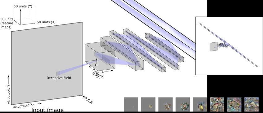
Figure 2 | The backpropagation algorithm. Backpropagation is an efficient algorithm for
computing how small adjustments to the connection weights affect the cost function that the
network is meant to minimize. A feedforward network with two hidden layers is shown as an
example. First, the activations are propagated in the feedforward direction (upward). The
activation function (gray sigmoid) is shown in each unit (circle). In the context of a particular input
pattern (not shown), the network is in a particular activation state, indicated by the black dots in
the units (horizontal axis: preactivation, vertical axis: activation). Second, the derivatives of the
cost function (squared-error cost shown on the right) are propagated in reverse (downward). In
the context of the present input pattern, the network can be approximated as a linear network
(black lines indicating the slope of the activation function). The chain rule defines how the cost
(the overall error) is affected by small changes to the activations, preactivations, and weights. The
goal is to compute the partial derivative of the cost with respect to each weight (bottom right).
Each weight is then adjusted in proportion to how much its adjustment reduces the cost. The
notation roughly follows Nielsen (2015), but we use bold symbols for vectors and matrices. The
symbol ⨀ denotes element-wise multiplication (Hadamard product).
We adjust each weight in the direction that reduces the cost (the error) and by an amount
proportional to the derivative of the cost with respect to the weight. This process is called
gradient descent, because it amounts to moving in the direction in weight space in which
the cost declines most steeply. To help our intuition, let us consider two approaches we
might take. First, consider the approach of taking a step to reduce the cost for each
individual training example. Gradient descent will make a minimal and selective
adjustments to reduce the error, which makes sense as we do not want learning from the
current example to interfere with what we’ve learned from other examples. However, our
goal is to reduce the overall error, which is defined as the sum of the errors across all
examples. So second, consider the approach of summing up the error surfaces (or,
equivalently, the gradients) across all examples before taking a step. We can still only
take a small step, because the error surface is nonlinear and so the gradient will change
as we move away from the point about which we linearized the network.
In practice, the best solution is to use small batches of training examples to estimate the
gradient before taking a step. Compared to the single-example approach, this gives us a
more stable sense of direction. Compared to the full-training-set approach, it greatly
6Kriegeskorte & Golan (2019) Neural network models and deep learning
reduces the computations required to take a step. Although the full-training-set approach
gives exact gradients for the training-set error, it still does not enable us to take large
steps, because of the nonlinearity of the error function. Using batches is a good
compromise between stability of the gradient estimate and computational cost. Because
the gradient estimate depends on the random sample of examples in the current batch,
the method is called stochastic gradient descent (SGD). Beyond the motivation just given,
the stochasticity is thought to contribute also to finding solutions that generalize well
beyond the training set (Poggio and Liao, 2017).
The cost is not a convex function of the weights, so we might be concerned about getting
stuck in local minima. However, the high dimensionality of weight space turns out to be a
blessing (not a curse) for gradient descent: there are many directions to escape in, making
it unlikely that we will ever find ourselves trapped, with the error surface rising in all
directions (Kawaguchi, 2016). In practice, it is saddle points (where the gradient vanishes)
that pose a greater challenge than local minima (Dauphin et al., 2014). Moreover, the
cost function typically has many symmetries, with any given set of weights having many
computationally equivalent twins (that is, the model computes the same overall function
for different parameter settings). As a result, although our solution may be one local
minimum among many, it may not be a poor local minimum: It may be one of many
similarly good solutions.
Recurrent neural networks are universal approximators of
dynamical systems
So far we have considered feedforward networks, whose directed connections do not
form cycles. Units can also be configured in recurrent neural networks (RNNs), where
activity is propagated in cycles, as is the case in brains (Dayan and Abbott, 2001;
Goodfellow et al., 2016). This enables a network to recycle its limited computational
resources over time and perform a deeper sequence of nonlinear transformations. As a
result, RNNs can perform more complex computations than would be possible with a
single feedforward sweep through the same number of units and connections.
For a given state space, a suitable RNN can map each state to any desired successor
state. RNNs, therefore, are universal approximators of dynamical systems (Schäfer and
Zimmermann, 2006). They provide a universal language for modeling dynamics, and one
whose components could plausibly be implemented with biological neurons.
Much like feedforward neural networks, RNNs can be trained by backpropagation.
However, backpropagation must proceed through the cycles in reverse. This process is
called backpropagation through time. An intuitive way to understand an RNN and
backpropagation through time is to ‘unfold’ the RNN into an equivalent feedforward
network (Figure 3). Each layer of the feedforward network represents a timestep of the
RNN. The units and weights of the RNN are replicated for each layer of the feedforward
network. The feedforward network, thus, shares the same set of weights across its layers
(the weights of the recurrent network).
7Kriegeskorte & Golan (2019) Neural network models and deep learning
Figure 3 | Recurrent neural networks. (a) A recurrent neural network models with two input
units (in blue box), three hidden units (green box), and two output units (pink box). The hidden
units here are fully recurrently connected: each sends its output to both other units. The arrows
represent scalar weights between particular units. (b) Equivalent feedforward network. Any
recurrent neural network can be unfolded along time as a feedforward network. To this end, the
units of the recurrent neural network (blue, green, pink sets) are replicated for each time step.
The arrows here represent weights matrices between sets of units in the colored boxes. For the
equivalence to hold, the feedforward network has to have a depth matching the number of time
steps that the recurrent network is meant to run for. Unfolding leads to a representation that is
less concise, but easier to understand and often useful in software implementations of recurrent
neural networks. Training of the recurrent model by backpropagation through time is equivalent
to training of the unfolded model by backpropagation.
For tasks that operate on independent observations (for example, classifying still images),
the recycling of weights can enable an RNN to perform better than a feedforward network
with the same number of parameters (Spoerer et al., 2017). However, RNNs really shine
in tasks that operate on streams of dependent observations. Because RNNs can maintain
an internal state (memory) over time and produce dynamics, they lend themselves to
tasks that require temporal patterns to be recognized or generated. These include the
perception speech and video, cognitive tasks that require maintaining representations of
hidden states of the agent (such as goals) or the environment (such as currently hidden
objects), linguistic tasks like the translation of text from one language into another, and
control tasks at the level of planning and selecting actions, as well as at the level of motor
control during execution of an action under feedback from the senses.
Deep neural networks provide abstract process models of
biological neural networks
Cognitive models capture aspects of brain information processing, but do not speak to its
biological implementation. Detailed biological models can capture the dynamics of action
potentials and the spatiotemporal dynamics of signal propagation in dendrites and axons.
However, they have only had limited success in explaining how these processes
contribute to cognition. Deep neural network models, as discussed here, strike a balance,
explaining feats of perception, cognition, and motor control in terms of networks of units
that are highly abstracted, but could plausibly be implemented with biological neurons.
For engineers, artificial deep neural networks are a powerful tool of machine learning. For
neuroscientists, these models offer a way of specifying mechanistic hypotheses on how
cognitive functions may be carried out by brains (Kriegeskorte and Douglas, 2018;
Kietzmann et al., 2019; Storrs and Kriegeskorte, in press). Deep neural networks provide
8Kriegeskorte & Golan (2019) Neural network models and deep learning
a powerful language for expressing information-processing functions. In certain domains,
they already meet or surpass human-level performance (for example, visual object
recognition and board games) while relying exclusively on operations that are biologically
plausible.
Neural network models in engineering have taken inspiration from brains, far beyond the
general notion that computations involve a network of units, each of which nonlinearly
combines multiple inputs to compute a single output (Kriegeskorte, 2015; Yamins and
DiCarlo, 2016). For example, convolutional neural networks (Fukushima and Miyake,
1982; LeCun et al., 1989), the dominant technology in computer vision, use a deep
hierarchy of retinotopic layers whose units have restricted receptive fields. The networks
are convolutional in that weight templates are automatically shared across image
locations (rendering the computation of a feature map’s preactivations equivalent to a
convolution of the input with the weight template). Although the convolutional aspect may
not capture an innate characteristic of the primate visual system, it does represent an
idealization of the final product of development and learning in primates, where
qualitatively similar features are extracted all over retinotopic maps at early stages of
processing. Across layers, these networks transform a visuospatial representation of the
image into a semantic representation of its contents, successively reducing the spatial
detail of the maps and increasing the number of semantic dimensions (Figure 4).
The fact that a neural network model was inspired by some abstract features of biology
and that it matches overall human or animal performance at a task, does not make it a
good model of how the human or animal brain performs the task. However, we can
compare neural network models to brains in terms of detailed patterns of behavior, such
as errors and reaction times for particular stimuli. Moreover, we can compare the internal
representations in neural networks to those in brains.
In the ‘white-box’ approach, we evaluate a model by looking at its internal representations.
Neural network models form the basis for predicting representations in different brain
regions for a particular set of stimuli (Diedrichsen and Kriegeskorte, 2017). One approach
is called encoding models. In encoding models, the brain activity pattern in some
functional region is predicted using a linear transformation of the representation in some
layer of the model (Kay et al., 2008; Mitchell et al., 2008). In another approach, called
representational similarity analysis (Kriegeskorte et al., 2008; Nili et al., 2014;
Kriegeskorte and Diedrichsen, 2016), each representation in brain and model is
characterized by a representational dissimilarity matrix. Models are evaluated according
to their ability to explain the representational dissimilarities across pairs of stimuli. A third
approach is pattern component modeling (Diedrichsen et al., 2011, 2017), where
representations are characterized by the second moment of the activity profiles.
Recent results from the domain of visual object recognition indicate that deep
convolutional neural networks are the best available model of how the primate brain
achieves rapid recognition at a glance, although they do not explain all of the explainable
variance in neuronal responses. (Cadieu et al., 2014; Khaligh-Razavi and Kriegeskorte,
2014; Yamins et al., 2014; Güçlü and van Gerven, 2015; Cichy et al., 2016; Eickenberg
et al., 2017; Wen et al., 2017; Nayebi et al., 2018), and yet multiple functional
incompatibilities have already been reported (Szegedy et al., 2013; Geirhos et al., 2017;
Jo and Bengio, 2017; Rajalingham et al., 2018).
9Kriegeskorte & Golan (2019) Neural network models and deep learning
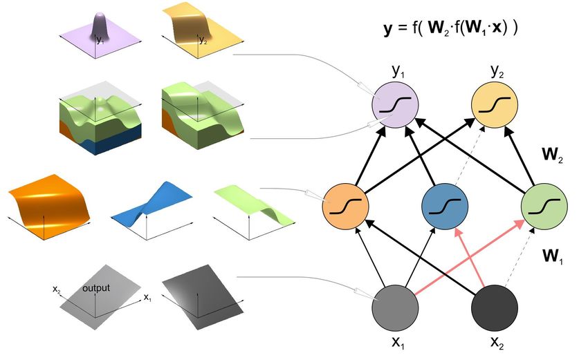
Figure 4 | Deep convolutional feedforward neural networks. The general structure of Alexnet,
a convolutional deep neural network architecture which had a critical role in bringing deep neural
networks into the spotlight. Unlike the visualization in the original report on this model, here the
tensors' dimensions are drawn to scale, so it is easier to appreciate how the convolutional deep
neural network gradually transforms the input image from a spatial to semantic representation.
For sake of simplicity, we did not visualize the pooling operations, as well as the splitting of some
of these layers between two GPUs. The leftmost box is the input image, (a tensor of the
dimensions 227×227×3, where 227 is the length of the square input-image edges and three is the
number of color components). It is transformed by convolution into the first layer (second box from
the left), a tensor with smaller spatial dimensions (55×55) but a larger number of feature maps
(96). Each feature map in this tensor is produced by a convolution of the original image with a
particular 11×11×3 filter. Therefore, the preactivation of each unit in this layer is a linear
combination of one rectangular receptive field in the image. The boundaries of such a receptive
field are visualized as a small box within the image tensor. In the next, second layer, the
representation is even more spatially smaller (27×27) but richer with respect of the number of
feature maps (256). Note that from here and onwards, each feature is not a linear combination of
pixels but a linear combination of the previous layer's features. The sixth layer (see the small
overview inset at the top-right) combines all feature maps and locations of the fifth layer to yield
4096 different scalar units, each with its own unrestricted input weights vector. The final eighth
layer has 1000 units, one for each output class. The eight images on the bottom were produced
by gradually modifying random noise images so excite particular units in each of the eight layers
(Erhan et al., 2009). The rightmost image was optimized to activate the output neuron related to
the class 'Mosque'. Importantly, these are only local solutions to the activation-maximization
problem. Alternative activation-maximizing images may be produced by using different starting
conditions or optimization heuristics.
In the ‘black-box’ approach, we evaluate a model on the basis of its behavior. We can
reject models for failing to explain detailed patterns of behavior. This has already helped
reveal some limitations of convolutional neural networks, which appear to behave
differently from humans under noisy conditions (Geirhos et al., 2017) and to show
different patterns of failures across exemplars (Rajalingham et al., 2018).
Deep neural networks bridge the gap between neurobiology and cognitive function,
providing an exciting framework for modeling brain information processing. Theories of
how the brain computes can now be subjected to rigorous tests by simulation. Our
10Kriegeskorte & Golan (2019) Neural network models and deep learning
theories, and the models that implement them, will evolve as we learn to explain the rich
measurements of brain activity and behavior provided by modern technologies in animals
and humans.
References
Cadieu CF, Hong H, Yamins DLK, Pinto N, Ardila D, Solomon EA, Majaj NJ, DiCarlo JJ
(2014) Deep neural networks rival the representation of primate IT cortex for core
visual object recognition. PLoS Comput Biol 10:e1003963.
Cichy RM, Khosla A, Pantazis D, Torralba A, Oliva A (2016) Comparison of deep neural
networks to spatio-temporal cortical dynamics of human visual object recognition
reveals hierarchical correspondence. Sci Rep 6:27755.
Cortes C, Vapnik V (1995) Support-vector networks. Mach Learn 20:273–297.
Cybenko G (1989) Approximation by superpositions of a sigmoidal function. Math Control
Signals Systems 2:303–314.
Dauphin YN, Pascanu R, Gulcehre C, Cho K, Ganguli S, Bengio Y (2014) Identifying and
Attacking the Saddle Point Problem in High-dimensional Non-convex Optimization.
In: Proceedings of the 27th International Conference on Neural Information
Processing Systems - Volume 2, pp 2933–2941 NIPS’14. Cambridge, MA, USA: MIT
Press.
Dayan P, Abbott LF (2001) Chapter 7.4, Recurrent Neural networks. In: Theoretical
neuroscience. Cambridge, MA: MIT Press.
Diedrichsen J, Kriegeskorte N (2017) Representational models: A common framework for
understanding encoding, pattern-component, and representational-similarity
analysis. PLoS Comput Biol 13:e1005508.
Diedrichsen J, Ridgway GR, Friston KJ, Wiestler T (2011) Comparing the similarity and
spatial structure of neural representations: a pattern-component model. Neuroimage
55:1665–1678.
Diedrichsen J, Yokoi A, Arbuckle SA (2017) Pattern component modeling: A flexible
approach for understanding the representational structure of brain activity patterns.
Neuroimage Available at: http://dx.doi.org/10.1016/j.neuroimage.2017.08.051.
Eickenberg M, Gramfort A, Varoquaux G, Thirion B (2017) Seeing it all: Convolutional
network layers map the function of the human visual system. Neuroimage 152:184–
194.
Erhan D, Bengio Y, Courville A, Vincent P (2009) Visualizing higher-layer features of a
deep network. University of Montreal 1341:1.
Fukushima K, Miyake S (1982) Neocognitron: A Self-Organizing Neural Network Model
for a Mechanism of Visual Pattern Recognition. In: Competition and Cooperation in
Neural Nets, pp 267–285. Springer Berlin Heidelberg.
Geirhos R, Janssen DHJ, Schütt HH, Rauber J, Bethge M, Wichmann FA (2017)
Comparing deep neural networks against humans: object recognition when the signal
gets weaker. arXiv [csCV] Available at: http://arxiv.org/abs/1706.06969.
11Kriegeskorte & Golan (2019) Neural network models and deep learning
Goodfellow I, Bengio Y, Courville A (2016) Deep Learning. MIT Press.
Goodfellow I, Pouget-Abadie J, Mirza M, Xu B, Warde-Farley D, Ozair S, Courville A,
Bengio Y (2014) Generative Adversarial Nets. In: Advances in Neural Information
Processing Systems 27 (Ghahramani Z, Welling M, Cortes C, Lawrence ND,
Weinberger KQ, eds), pp 2672–2680. Curran Associates, Inc.
Güçlü U, van Gerven MAJ (2015) Deep Neural Networks Reveal a Gradient in the
Complexity of Neural Representations across the Ventral Stream. J Neurosci
35:10005–10014.
Hinton GE, Salakhutdinov RR (2006) Reducing the dimensionality of data with neural
networks. Science 313:504–507.
Hornik K, Stinchcombe M, White H (1989) Multilayer feedforward networks are universal
approximators. Neural Netw 2:359–366.
Jo J, Bengio Y (2017) Measuring the tendency of CNNs to Learn Surface Statistical
Regularities. arXiv [csLG] Available at: http://arxiv.org/abs/1711.11561.
Kawaguchi K (2016) Deep Learning without Poor Local Minima. In: Advances in Neural
Information Processing Systems 29 (Lee DD, Sugiyama M, Luxburg UV, Guyon I,
Garnett R, eds), pp 586–594. Curran Associates, Inc.
Kay KN, Naselaris T, Prenger RJ, Gallant JL (2008) Identifying natural images from
human brain activity. Nature 452:352–355.
Khaligh-Razavi S-M, Kriegeskorte N (2014) Deep supervised, but not unsupervised,
models may explain IT cortical representation. PLoS Comput Biol 10:e1003915.
Kietzmann TC, McClure P, Kriegeskorte N (2019) Deep Neural Networks in
Computational Neuroscience. Available at:
http://oxfordre.com/neuroscience/view/10.1093/acrefore/9780190264086.001.0001/
acrefore-9780190264086-e-46.
Kriegeskorte N (2015) Deep Neural Networks: A New Framework for Modeling Biological
Vision and Brain Information Processing. Annu Rev Vis Sci 1:417–446.
Kriegeskorte N, Diedrichsen J (2016) Inferring brain-computational mechanisms with
models of activity measurements. Philos Trans R Soc Lond B Biol Sci 371 Available
at: http://dx.doi.org/10.1098/rstb.2016.0278.
Kriegeskorte N, Douglas PK (2018) Cognitive computational neuroscience. Nat Neurosci
21:1148–1160.
Kriegeskorte N, Mur M, Bandettini P (2008) Representational similarity analysis -
connecting the branches of systems neuroscience. Front Syst Neurosci 2:4.
Krizhevsky A, Sutskever I, Hinton GE (2012) ImageNet Classification with Deep
Convolutional Neural Networks. In: Advances in Neural Information Processing
Systems 25 (Pereira F, Burges CJC, Bottou L, Weinberger KQ, eds), pp 1097–1105.
Curran Associates, Inc.
LeCun Y, Bengio Y, Hinton G (2015) Deep learning. Nature 521:436.
LeCun Y, Boser B, Denker JS, Henderson D, Howard RE, Hubbard W, Jackel LD (1989)
Backpropagation Applied to Handwritten Zip Code Recognition. Neural Comput
12Kriegeskorte & Golan (2019) Neural network models and deep learning
1:541–551.
Lin HW, Tegmark M, Rolnick D (2017) Why Does Deep and Cheap Learning Work So
Well? J Stat Phys 168:1223–1247.
McCulloch WS, Pitts W (1943) A logical calculus of the ideas immanent in nervous
activity. Bull Math Biophys 5:115–133.
Mitchell TM, Shinkareva SV, Carlson A, Chang K-M, Malave VL, Mason RA, Just MA
(2008) Predicting human brain activity associated with the meanings of nouns.
Science 320:1191–1195.
Mnih V, Kavukcuoglu K, Silver D, Rusu AA, Veness J, Bellemare MG, Graves A,
Riedmiller M, Fidjeland AK, Ostrovski G, Petersen S, Beattie C, Sadik A, Antonoglou
I, King H, Kumaran D, Wierstra D, Legg S, Hassabis D (2015) Human-level control
through deep reinforcement learning. Nature 518:529.
Nayebi A, Bear D, Kubilius J, Kar K, Ganguli S, Sussillo D, DiCarlo JJ, Yamins DL (2018)
Task-Driven convolutional recurrent models of the visual system. In: Advances in
Neural Information Processing Systems, pp 5295–5306.
Nielsen MA (2015) Neural networks and deep learning. Determination Press.
Nili H, Wingfield C, Walther A, Su L, Marslen-Wilson W, Kriegeskorte N (2014) A toolbox
for representational similarity analysis. PLoS Comput Biol 10:e1003553.
Poggio T, Liao Q (2017) Theory ii: Landscape of the empirical risk in deep learning.
Rajalingham R, Issa EB, Bashivan P, Kar K, Schmidt K, DiCarlo JJ (2018) Large-scale,
high-resolution comparison of the core visual object recognition behavior of humans,
monkeys, and state-of-the-art deep artificial neural networks. bioRxiv:240614
Available at: https://www.biorxiv.org/content/early/2018/01/01/240614 [Accessed
April 16, 2018].
Rolnick D, Tegmark M (2017) The power of deeper networks for expressing natural
functions. arXiv [csLG] Available at: http://arxiv.org/abs/1705.05502.
Rosenblatt F (1958) The perceptron: a probabilistic model for information storage and
organization in the brain. Psychol Rev 65:386–408.
Rumelhart DE, Hinton GE, Williams RJ (1986) Parallel Distributed Processing:
Explorations in the Microstructure of Cognition, Vol. 1. In (Rumelhart DE, McClelland
JL, PDP Research Group C, eds), pp 318–362. Cambridge, MA, USA: MIT Press.
Rumelhart DE, McClelland JL, Group PR, Others (1987) Parallel distributed processing.
MIT press Cambridge, MA.
Schäfer AM, Zimmermann HG (2006) Recurrent Neural Networks Are Universal
Approximators. In: Artificial Neural Networks -- ICANN 2006 (Kollias SD, Stafylopatis
A, Duch W, Oja E, eds), pp 632–640. Berlin, Heidelberg: Springer Berlin Heidelberg.
Schmidhuber J (2015) Deep learning in neural networks: An overview. Neural Netw
61:85–117.
Schölkopf B, Smola AJ (2002) Learning with Kernels: Support Vector Machines,
Regularization, Optimization, and Beyond. MIT Press.
Spoerer CJ, McClure P, Kriegeskorte N (2017) Recurrent Convolutional Neural Networks:
13Kriegeskorte & Golan (2019) Neural network models and deep learning
A Better Model of Biological Object Recognition. Front Psychol 8:1551.
Stanley KO, Clune J, Lehman J, Miikkulainen R (2019) Designing neural networks
through neuroevolution. Nature Machine Intelligence 1:24–35.
Storrs KR, Kriegeskorte N (in press.) Deep learning for cognitive neuroscience. In: The
Cognitive Neurosciences (6th Edition). (Gazzaniga M, ed). Boston: MIT Press.
Such FP, Madhavan V, Conti E, Lehman J, Stanley KO, Clune J (2017) Deep
Neuroevolution: Genetic Algorithms Are a Competitive Alternative for Training Deep
Neural Networks for Reinforcement Learning. arXiv [csNE] Available at:
http://arxiv.org/abs/1712.06567.
Szegedy C, Zaremba W, Sutskever I, Bruna J, Erhan D, Goodfellow I, Fergus R (2013)
Intriguing properties of neural networks. arXiv [csCV] Available at:
http://arxiv.org/abs/1312.6199.
Wen H, Shi J, Zhang Y, Lu K-H, Cao J, Liu Z (2017) Neural Encoding and Decoding with
Deep Learning for Dynamic Natural Vision. Cereb Cortex:1–25.
Werbos PJ (1982) Applications of advances in nonlinear sensitivity analysis. In: System
Modeling and Optimization, pp 762–770. Springer Berlin Heidelberg.
Yamins DLK, DiCarlo JJ (2016) Using goal-driven deep learning models to understand
sensory cortex. Nat Neurosci 19:356–365.
Yamins DLK, Hong H, Cadieu CF, Solomon EA, Seibert D, DiCarlo JJ (2014)
Performance-optimized hierarchical models predict neural responses in higher visual
cortex. Proc Natl Acad Sci 111:8619–8624.
14You can also read