PHOTOVOLTAIC SOLAR ENERGY CONVERSION - Tom Markvart School of Engineering Sciences University of Southampton Southampton SO17 1BJ, UK - European ...
←
→
Page content transcription
If your browser does not render page correctly, please read the page content below
PHOTOVOLTAIC SOLAR ENERGY
CONVERSION

Tom Markvart

School of Engineering Sciences
University of Southampton
Southampton SO17 1BJ, UK

European Summer University: Energy for Europe
Strasbourg, 7-14 July 2002
1. INTRODUCTION

This lecture gives an overview of photovoltaics: the direct conversion of light into
electricity.The usage of solar energy for heat has a long history but the origin of devices
which produce electricity is much more recent: it is closely linked to modern solid-state
electronics. Indeed, the first usable solar cell was invented at Bell Laboratories – the
birthplace of the transistor - in the early 1950’s.

The first solar cells found a ready application in supplying electrical power to satellites.
Terrestrial systems soon followed; these were what we would now call remote industrial
or professional applications, providing small amounts of power in inaccessible and
remote locations, needing little or no maintenance or attention. Examples of such
applications include signal or monitoring equipment, or telecommunication and
corrosion protection systems. Since then, numerous photovoltaic systems have been
installed to provide electricity to the large number of people on our planet that do not
have (nor, in the foreseeable future, are likely to have) access to mains electricity.
Power supply to remoter houses or villages, lighting, electrification of the healthcare
facilities, irrigation and water supply and treatment will form an important application
of photovoltaics for many years to come. In the recent years, production of solar cells
has been growing by 30% a year, reaching almost 400MW in 2001 (Fig. 1.1). Perhaps
the most exciting new application has been the integration of solar cells into the roofs
and facades of buildings during the last decade of the 20th century providing a new,
distributed, form of power generation (see Table 1).

In this lecture, we shall look at a three aspects of this new and rapidly growing energy
technology. The properties of solar radiation as an energy source will be summarised in
Sec. 2. Sections 3 and 4 give an overview of the operation of solar cells, focusing on the
quantum-mechanical aspects of the conversion process, and providing a link to other,
fundamentally similar but seemingly quite disparate, conversion systems such as the
primary chemical reaction in photosynthesis. Section 5 concludes with a summary of
the system aspects.

     1950s           First modern solar cells
     1960s           Solar cells become main source of electric power for satellites
     1970s           First remote industrial applications on the ground
     1980s           Solar cells used in rural electrification and water pumping.
                     First grid connected systems
     1990s           Major expansion in building-integrated systems
     2000s           ???

Table 1. A brief history of photovoltaic applications

                                             1
400
PV Power
Grid-connected: stations 2% Consumer
World solar cell production (MWp)
distributed products
21% 20%
300
PV/diesel
hybrids
13% Stand alone:
rural &domestic
Professional
22%
applications
22%
200
100
0
1991 1992 1993 1994 1995 1996 1997 1998 1999 2000 2001
Fig. 1.1 World solar cell production and the main photovoltaic markets (source: Paul
Maycock, PV News)
2. SOLAR RADIATION
To a good approximation, the sun acts as a perfect emitter of radiation (black body).
The resulting (average) energy flux incident on a unit area perpendicular to the beam
outside the Earth's atmosphere is known as the solar constant:
S = 1367 W/m 2 (1)
In general, the total power from a radiant source falling on a unit area is called
irradiance.
The black-body temperature of solar radiation which agrees with the value of S (1) can
be obtained from the Stefan-Boltzmann law and a simple geometrical argument
involving the Sun-Earth distance RSE and the radius of the Sun RS:
S = fω σ TS4
where the geometrical factor fω is given by
2
R
fω = S (2)
R SE
The solid angle ωS subtended by the Sun, related to fω by fω = ωS/π, is also sometimes
used. The concept of black body radiation makes it possible to use the Planck’s
2radiation formula for the photon flux received by a planar surface of unit area in a
frequency interval ν Æ ν + δν:
2π ν 2 δν 2π hν
2 − k B TS
δφ = f ω hν
≅ f ω ν e δν (3)
c 2 e kTS − 1 c 2
where h is the Planck constant, c is the speed of light in vacuum, and kB is the
Boltzmann constant.
When the solar radiation enters the Earth's atmosphere, a part of the incident energy is
removed by scattering or absorption by air molecules, clouds and particulate matter
usually referred to as aerosols. The radiation that is not reflected or scattered and
reaches the surface directly in line from the solar disc is called direct or beam radiation.
The scattered radiation which reaches the ground is called diffuse radiation. Some of
the radiation may reach a receiver after reflection from the ground, and is called the
albedo. The total radiation consisting of these three components is called global.
The amount of radiation that reaches the ground is, of course, extremely variable. In
addition to the regular daily and yearly variation due to the apparent motion of the Sun,
irregular variations are caused by the climatic conditions (cloud cover), as well as by
the general composition of the atmosphere. For this reason, the design of a photovoltaic
system relies on the input of measured data close to the site of the installation.
A concept which characterises the effect of a clear atmosphere on sunlight is the air
mass, equal to the relative length of the direct beam path through the atmosphere. On a
clear summer day at sea level, the radiation from the sun at zenith corresponds to air
mass 1 (abbreviated to AM1); at other times, the air mass is approximately equal to
1/cos θ , where θ is the zenith angle.
250
200
spectral irradiance, mW/cm 2µm
AM0
black body, T = 5762K
AM1.5 normalised
150
100
50
0
0 0.5 1 1.5 2 2.5 3 3.5 4
wavelength, µm
Fig. 2.1. Solar spectra commonly used in photovoltaics
3The effect of the atmosphere (as expressed by the air mass) on the solar spectrum is
shown in Fig. 2.1. The extraterrestrial spectrum, denoted by AM0, is important for
satellite applications of solar cells. AM1.5 is a typical solar spectrum on the Earth's
surface in a clear day which, with total irradiance of 1 kW/m2, is used for the calibration
of solar cells and modules.
Instead of irradiance, the design of photovoltaic systems (particularly stand-alone ones)
is usually based on daily solar radiation: the energy received by a unit area in one day.
An idea of how large quantity this is can be obtained as follows. The total energy flux
incident on the Earth is equal to S multiplied by the area of the disk presented to the
Sun’s radiation by the Earth. The average flux incident on a unit surface area is then
obtained by dividing this number by the total surface area of the Earth. Making
allowance for 30% of the incident radiation being scattered and reflected into space, the
average daily solar radiation G on the ground is equal to
πR E2 1
G = 24 x0.7 x x S = 24 x0.7 x S = 5.74 kWh (4)
4πR 2
E
4
where RE is the radius of the Earth. This number should be compared with the observed
values. Figure 2.2 shows the daily solar radiation on a horizontal plane for four
locations ranging from the tropical forests to northern Europe. The solar radiation is
highest in the continental desert areas around latitude 25 N and 25 S, and falls off
towards the equator because of the cloud, and towards the poles because of low solar
elevation. Equatorial regions experience little seasonal variation, in contrast with higher
latitudes where the summer/winter ratios are large.
9
8
7
2
Daily solar radiation, kWh/m
6
5
4
3
Sahara desert
2 Almeria, Spain
South Vietnam (tropical)
1 London, UK
0
Jan Feb Mar Apr May Jun Jul Aug Sep Oct Nov Dec
Fig. 2.2 Mean daily solar radiation in different parts of the world. The daily radiation in
kWh/m2, sometimes called ‘Peak Solar Hours’, is of fundamental importance in
photovoltaic system design (see Sec. 5). The dashed line shows the average value (4).
43. TWO-LEVEL QUANTUM ENERGY CONVERTER
It will be useful to consider a simple model of the
energy conversion process which illustrates the
principles, namely the detailed balance between
energy of the absorbed light and the free energy
delivered to the user. The main part of the con-
version system (Fig. 3.1) is a light absorber with
two quantum states where the absorption of a ∆E τ g+g0
photon of light promotes an electron from the
ground state to an excited state. The rate of
excitation is a combination of two processes,
illumination (inducing transitions with rate g) and hν
thermal excitation, with rate go. The lifetime of
the excited state with respect to transitions to the
Fig. 3.1
ground state will be denoted by τ.
Let us denote by (1-q) and p the probabilities that the absorber is in ground and excited
state, respectively. The quantity q can be interpreted as the hole occupation probability
of the ground state. The rates of excitation and de-excitation then are
1
R = pq
τ (5)
G = (g + g o )(1 − p)(1 − q)
In thermal equilibrium when g=0, the thermal generation rate is equal to the excitation
rate, and go can be expressed in terms of the equilibrium values of po and qo at the
ambient temperature T:
∆E
1 po qo 1 −
go = = e kBT (6)
τ 1 − p o 1 − qo τ
This is just another way of writing Einstein’s famous relation between the A and B
coefficients.
The conversion processes is now modelled by adding two other states: an electron
reservoir (which accepts an electron from the excited state) and a hole reservoir (which
accepts a 'hole' from the ground state or, in other words, donates an electron to the
ground state, Fig. 3.2). In steady state, the rate of energy extraction (denoted by K) is
equal to the rate of transfer of electrons and holes to the reservoirs which, in turn, must
be equal to the net excitation rate:
1
K =G − R =(g + g o )(1 − p)(1 − q) − pq (7)
τ
5In different applications, the rate K might be the rate of a photochemical redox reaction
which proceeds by electron transfer from redox couple 1 (denoted by D-/D, where D
stands for electron donor) to redox couple 2 (A-/A, where A denotes electron acceptor):
D − + A→ D + A − (8)
The two terms G and R then correspond to the forward and reverse reaction (8). In a
solar cell, the rate K is related to the current in the external circuit I by
I = qK (9)
where q (>0) is the electron charge.
The free energy per electron in the two reservoirs (in other words, the chemical
potentials) will be denoted by µe and µh. In thermal equilibrium µe = µh but in general,
µe and µh will not be equal, and an amount of external work equal to ∆µ = µe - µh can be
carried out by transferring an electron from the electron to the hole reservoir. This
electron transfer models a chemical redox reaction or, as we shall see in the next
section, the electrical current in an external circuit.
µe
∆µ
µh
hν
Fig. 3.2 The quantum energy converter
If the transitions between the two quantum levels and the reservoirs are reversible to
ensure maximum energy extraction, the free energy of electron in the excited and
ground states are equal to µe and µh, and the populations p and 1-q follow the Fermi-
Dirac distribution
1 1
p= ; 1− q = (10)
E − µe Eg − µh
1 + exp exc 1 + exp
kBT kBT
Substituting (10) into (7) then gives
6 1 − k B T − k B T
∆E ∆µ
K = (1 − q)(1 − p)g − e e − 1 (11)
τ
where ∆E = Eexc-Eg. The two factors outside the braces may become relevant under very
strong illumination but under modest excitation which we shall consider here, p,qThe model that we have just described can be generalised to include the situation where
the electron transfer from the hole to electron reservoir takes place in an electric field
with electrostatic potential ψ which has the value ψe in the electron reservoir and ψh in
the hole reservoir. The conversion equation (12) then remains in force but the chemical
potential difference ∆µ =µe - µh must be replaced by the difference ∆φ of electro-
chemical potentials φe = µe - qψe and φh = µh - qψh.. This will be particularly relevant in
the case of solar cell which will be discussed in Sec. 4. We shall see that if the rates K
are replaced by the appropriate electrical currents and ∆φ by qV = q(ψe - ψh) = ∆ψ,
where V is the voltage at the terminals of the cell, Eq. (12) becomes the Shockley's
ideal solar cell equation.
In addition to semiconductor solar cells, the two level converter serves as a model for a
number of other quantum solar energy conversion systems. Two of these are briefly
discussed below.
The primary photochemical reaction in photosynthesis
The fundamental photosynthetic reaction can be represented by electron transport across
the photosynthetic membrane. The reaction is responsible for the formation of high-
energy chemical products and, in some organisms, electrostatic potential can also form
across the membrane. The electron transport takes place in the photosynthetic reaction
centre - a protein complex which binds components of the electron transport chain
shown in Fig. 3.3. The primary electron donor (usually denoted by P) is a chlorophyll
(or bacteriochlorophyll) dimer. The electron transport then proceeds through a number
of intermediaries to a quinone molecule Q. Electron excitation by light from the ground
state of P to an excited state P* is followed by electron transfer to Q, creating the
reduced form Q-. The reduced quinone Q- is subsequently oxidised to Q by an
extraneous electron acceptor, the ground state of the primary donor is replenished by an
electron, and the electron transfer cycle can start again. The link to the two level
quantum energy converter is apparent from Fig. 3.3 b which can be used to estimate
thermodynamic limits on the conversion efficiency (Ross and Calvin, 1967).
periplasm P*
+
Electric field
BB BA P+ Q-
P bacterial
HB HA membrane
Fe
- QB QA
cytoplasm
P
(a) (b)
Fig. 3.3 A schematic diagram of the photosynthetic reaction centre in purple bacteria
(a). The electron transport can be modelled in a simplified manner by a scheme shown
in (b). In reality, the primary donor P is rarely excited directly by the incident light but
the excitation proceeds via an ‘antenna’ of accessory bacteriochlorophyll molecules
which transfer the excitation energy to P by resonant energy transfer.
8Dye sensitised solar cells. Invented by Michael Grätzel and his group at the Ecole
Polytechnique Fédérale de Lausanne in the early 1990s, these cells were arguably the
first photochemical solar cells that operate on a similar principle as the photosynthetic
conversion system. Molecules of Ru-based dye, deposited on very small (‘nano-
crystalline’) particles of titanium dioxide act as the absorber in the quantum energy
converter (Fig. 3.4). Electrons, supplied to the ground state of the dye from a liquid
redox iodine/ iodide electrolyte are transferred, upon photoexcitation, from the excited
state of the dye to the conduction band of TiO2 (Fig. 3.5). In effect, the mono-molecular
dye layer ‘pumps’ electrons from one electrode (liquid electrolyte) to the other (solid
titanium dioxide). The use of nanocrystalline TiO2 particles coated by the dye ensures
high optical absorption, resulting in almost all light within the spectral range of the dye
being absorbed by a coating not more than few angstroms thin.
Dye-coated
TiO2
redox
electrolyte
Back contact Front contact
(TCO coated (TCO coated
glass) glass)
Fig. 3.4 Cross section of the dye sensitised cell.
e- (S+/ S*)
hν e-
(I -/I3-)
(S+/S)
e- e-
TiO2
load
e-
Fig. 3.5 The energy diagram of the electron flow in the dye sensitised cell. The ground,
excited and oxidised states of the dye molecule are denoted by S, S* and S+,
respectively. After A. Mc Evoy, Electrochemical photovoltaics, p. 247 in: T. Markvart,
Solar Electricity (see bibliography).
94. SEMICONDUCTOR SOLAR CELLS
Solar cell operation
The operation of a semiconductor solar cell will be illustrated on the example of a p-n
junction under illumination. The p-n junction is effectively an interface between n and p
type semiconductors: in other words, semiconductor where excess electrons and holes have
been introduced by the addition of impurities. The fundamental characteristic of the junction
is the presence of a strong electric field, indicated by the slope of the edges of the
conduction and valence band in the junction region (Fig. 4.1a).
Conduction band
n - type
semiconductor
hν
Eg φe
e∆ψ
φ
φh
p - type
semiconductor
Valence band
Electrical load
(a) (b)
Fig. 4.1 Semiconductor p-n junction in equilibrium (a) and under illumination (b).
In equilibrium, the electrochemical potentials on the two sides of the junction are equal, and
there is no net electric current. Under illumination, electron-hole pairs are generated in the
semiconductor, and are subsequently separated by the electric field of the junction
(Fig. 4.1b). A quick reflection shows that the p-n junction behaves as the quantum converter
discussed in Sec. 3, with the bandgap of the semiconductor Eg playing the role of the
excitation energy ∆E. Replacing now ∆µ by qV and the rates K by electrical currents I
using (9),
− kqVT
I = Il − Io e B − 1 (17)
The resulting I-V characteristic (17) is shown in Fig. 4.2. The photogenerated current Iℓ is
equal to the current produced by the cell at short circuit (V=0). The open circuit voltage
Voc (when I=0) can easily be obtained in a similar way as ∆µK=0 in Eq. (14):
k B T Il
Voc = ln1 + (18)
q Io
10No power is generated under short or open circuit. The maximum power P produced by the
conversion device is reached at a point on the characteristic where the product IV is
maximum. This is shown graphically in Fig. 4.2 where the position of the maximum power
point represents the largest area of the rectangle shown. One usually defines the fill-factor ff
by
Pmax VmIm
ff = = (19)
Voc I l Voc I l
where Vm and Im are the voltage and current at the maximum power point.
Isc Pmax
Current, A
Maximum power
rectangle
Voltage, V Voc
Fig. 4.2 The I-V characteristic of an ideal solar cell
The principal difference between a semiconductor solar cell and the the two level converter
of Sec. 3 lies in the nature of optical absorption of the semiconductor which occurs in a
broad spectral range rather than in a narrow spectral line. Indeed, a sufficiently thick slab
may absorb all photons with energy in excess of the semiconductor bandgap Eg. Neglecting
reflection and assuming that all the photogenerated electrons and holes are collected to
generate power, the photogenerated current will then be
∞
2π ν 2 dν
Il = A q ∫ δφ = A q fω
c 2 νg =∫Eg / h e kTS − 1
hν (20)
where A is the cell area and we made use of expression (3) for the black body photon flux
δφ. Note that the current (20) decreases with increasing bandgap since for larger
bandgaps, fewer photons have energies in excess of Eg and can be absorbed by the
semiconductor.
The open circuit voltage of an ideal solar cell can be obtained in a similar manner as in
the thermodynamic argument used to obtain ∆µK=0 in Eq. (16). Since absorption takes
place over a broader energy range than the room-temperature photon emission, a term
k B T ln(Ts / T ) can be added to improve the accuracy, giving
11Eg T kBT π k B T Ts
Voc = 1 − − ln + ln (21)
q TS q ω S q T
Figures 4.3 and 4.4 compare the theoretical predictions with the open circuit voltage and
short circuit of the best cells made from different materials. It is seen that the observed
values of short circuit current for several materials almost reach the theoretical maximum.
This corresponds to a virtually 100% quantum yield – in other words, almost every
photon gives rise to an electron in the external circuit. The open circuit voltage is more
sensitive to nonradiative recombination (to be discussed below) and the observed values
are slightly lower, although the difference in the case of crystalline materials is still less
than 20%.
80
70
60
50
Jsc (mA/cm )
2
c-Si
40
GaAs
CIGS
30
InP CdTe
20
a-Si
10
0
0 1 2 3 4
Eg (eV)
Fig. 4.3 The measured short circuit current for various materials compared with the
maximum theoretical value (full line). Full and empty symbols correspond to crystalline
and thin film materials, respectively.
1.4
Theoretical limit
1.2
Voc, V
1.0 GaAs
InP a-Si
0.8 CdTe
c-Si
CIGS
0.6
1 1.1 1.2 1.3 1.4 1.5 1.6 1.7 1.8
Eg, eV
Fig. 4.4 The measured open circuit voltage for various materials compared with the
maximum theoretical value. Full and empty symbols correspond to crystalline and thin
film materials, respectively.
12The quantity of greatest interest is the efficiency which can be obtained from (18) and
(20) with the use of the fill factor (19) which can be determined numerically as the
solution of
v m = v oc − ln( v m + 1) (22)
where voc=Voc/kT and vm=Vm/kT. The maximum theoretical efficiency is shown as a
function of the bandgap in Fig. 4.5 (Shockley and Queisser, 1961). The bandgaps of the
principal photovoltaic materials (to be discussed below) are also shown. The curve
marked ‘one sun’ corresponds to the usual terrestrial conditions, approximating the solar
radiation by the black body spectrum with temperature Ts = 6000K. To a good accuracy,
this curve can be obtained with the use of the open circuit voltage given by Eq. (21). The
curve marked ‘concentrated sunlight’ is plotted under conditions when solar radiation is
focused with lenses or mirrors, enhancing the efficiency. This can be seen from the
voltage equation (21) where, under maximum concentration, the second term effectively
drops out.
50%
cSi
CuInSe2 GaAs
40%
aSi
concentrated light
30%
Efficiency
InP
CdTe
20%
one sun
10%
0%
0 1 2 3 4 5
Eg (eV)
Fig. 4.5 The Shockley-Queisser limit to the efficiency of single junction solar cells.
Practical devices
Solar cells are now manufactured from a number of different semiconductors which are
summarised below. In addition, there is considerable activity to manufacture commercially
the dye sensitised solar cells which were discussed briefly in Sec. 3.
• Crystalline silicon cells dominate the photovoltaic market. To reduce the cost, these
cells are now often made from multicrystalline material, rather than from the more
expensive single crystals. Crystalline silicon cell technology is well established. The
modules have long lifetime (20 years or more) and their best production efficiency is
approaching 18%.
• Amorphous silicon solar cells are cheaper (but also less efficient) type of silicon cells,
made in the form of amorphous thin films which are used to power a variety of
consumer products but larger amorphous silicon solar modules are also becoming
available.
13• Cadmium telluride and copper indium diselenide thin-film modules are now
beginning to appear on the market and hold the promise of combining low cost with
acceptable conversion efficiencies.
• High-efficiency solar cells from gallium arsenide, indium phosphide or their derivatives
are used in specialised applications, for example, to power satellites or in systems which
operate under high-intensity concentrated sunlight.
The structure of a typical silicon solar cell is illustrated in Fig. 4.6. The electrical current
generated in the semiconductor is extracted by contacts to the front and rear of the cell. The
top contact structure which must allow light to pass through is made in the form of widely-
spaced thin metal strips (usually called fingers) that supply current to a larger bus bar
(Transparent conducting oxide is also used on a number of thin film devices). The cell is
covered with a thin layer of dielectric material - the antireflection coating, ARC - to
minimise light reflection from the top surface.
bus bar
finger
(top contact)
arc
emitter (n-type)
junction
base (p-type)
back contact
Fig. 4.6. The structure of a typical crystalline silicon solar cell.
The energy conversion process in solar cells is very different from the operation of the
classical heat engine, and it is instructive to consider the limitations and losses that occur
in more detail. The fundamental mechanisms responsible for losses in solar cells are
apparent from the discussion of solar cell operation earlier in this section: heat is
produced on carrier generation in the semiconductor by photons with energy in excess of
the bandgap, and a considerable part of the solar spectrum is not utilised because of the
inability of a semiconductor to absorb the below-bandgap light. These losses can be
reduced, but only going over to more complex structures based on several
semiconductors with different bandgaps. A device called tandem cell, for example,
represents effectively a stack of several cells each operating according to the principles
that we have just described. The top cell is made of a high-bandgap semiconductor, and
converts the short-wavelength radiation. The transmitted light is then converted by the
bottom cell. This arrangement increases considerably the achievable efficiency: high
14efficiency space cells operating at close to 30% are now commercially available. There
are also amorphous silicon cells where a double or triple stack is used to boost the low
efficiencies of single-junction devices and reduce the degradation which is observed in
these materials.
10 W
2.1 W no below-bandgap absorption
3.1 W excess photon energy lost as heat
Badgap energy 1.12 eV Current available 4.4 A
Fundamental
thermodynamic losses Losses in Non-PV absorption
Collection efficiency
0.86 V
semiconductor Incomplete absorption
Top-surface reflection
Nonradiative
recombination
solar cells Top-contact shading
Open circuit voltage Short-circuit current
0.58 (0.7) V 3.3 (4.2) A
Series resistance losses
Fill factor 0.75 (0.8)
Cell output 1.5 W (2.5 W)
Efficiency 15% (25%)
Fig. 4.7 The various losses in a semiconductor solar cell, shown here on the example of
100x100mm monocrystalline silicon cell. Figures are for production cells; best
experimental values in are in brackets.
Other losses reduce the typical efficiency of commercial devices to roughly 50% of the
achievable maximum (Fig. 4.7), somewhat less in thin-film devices. A ubiquitous loss
mechanisms present in all practical devices is non-radiative recombination of the
photogenerated electron-hole pairs. Such recombination is most common at impurities
and defects of the crystal structure, or at the surface of the semiconductor where energy
levels may be introduced inside the energy gap. These levels act as stepping stones for
the electrons to fall back into the valence band and recombine with holes. An important
site of recombination are also the ohmic metal contacts to the semiconductor. Measures
taken to minimise the recombination losses include careful processing to maintain long
minority-carrier lifetime, and protecting the external surfaces of the semiconductor by a
layer of passivating oxide to reduce surface recombination. The contacts can be
surrounded by heavily-doped regions acting as "minority-carrier mirrors" which impede
the minority carriers from reaching the contacts and recombining.
The losses to current by recombination are usually grouped under the term of collection
efficiency: the ratio between the number of carrier generated by light and the number that
reaches the junction. Considerations of the collection efficiency affect the design of the
solar cell. In crystalline materials, the transport properties are usually good, and carrier
transport by simple diffusion is sufficiently effective. In amorphous and polycrystalline
15thin films, however, electric fields are needed to pull the carriers. The junction region is
then made wider to absorb the main part of the photon flux.
Other losses to the current produced by the cell arise from light reflection from the top
surface, shading of the cell by the top contacts, and incomplete absorption of light. The
last feature can be particularly significant for crystalline silicon cells since silicon – being
an indirect-gap semiconductor - has poor light absorption properties. Measures which can
be taken to reduce these losses include the use of multi-layer antireflection coatings,
surface texturing to form small pyramids, and making the back contact optically
reflecting. When combined with a textured top surface, this geometry results in effective
light trapping which provides an good countermeasure for the low absorptivity of silicon.
Top-contact shading is reduced in some cells by forming these contacts in narrow laser
grooves, or all the contacts can be moved to the rear of the cell. Another common loss in
commercial cells involves ohmic losses in the transmission of electric current produced
by the solar cell, usually grouped together as a series resistance, which reduce the fill
factor of the cell.
The principal characteristics of different types of cell in or near commercial production
are summarised in Table 5.1.
Material Efficiency (%) Technology
Commercial products Best R&D
Mono- or multi-crystalline silicon 10-18 25 ingot/wafer
Amorphous silicon 5-8 13 thin film
Copper indium diselenide 8 16 thin film
Cadmium telluride 7 16 thin film
Table 5.1. Solar cell efficiencies achieved by the principal semiconductor technologies
We have already seen earlier in this section that, in addition to crystalline silicon, much
effort is focused on the manufacture of thin-film devices which have lower material
requirements. We have also seen, on the example of dye sensitised solar cell, that
photovoltaic materials are no longer restricted to semiconductors. Furthermore, there is
considerable research activity into purely molecular materials. A number of research
groups have demonstrated solar cells based on conducting polymers, often in
combination with fulerene derivatives as electron acceptors to create the p-n junction.
There is much to look forward to if their success matches the achievements of the LED
technology.
165. ISSUES IN SYSTEM DESIGN
For practical use, solar cells are laminated and encapsulated to form photovoltaic
modules. These are then combined into arrays, and interconnected with other electrical
and electronic components – for example, batteries, charge regulators and inverters - to
create a photovoltaic system. A number of issues need to be resolved before an optimum
system design is achieved. These issues include the choice between a flat plate or
concentrating system, and whether fixed tilt will be used or the modules will ‘track’ the
sun. Answers to these questions will vary depending on the solar radiation at the site of
the installation and its variation during the year (see Fig. 2.1). Specific issues also relate
to whether the system is to be connected to the utility supply (the ‘grid’) or is intended for
stand-alone operation.
Most photovoltaic arrays are installed at fixes tilt and, wherever possible, oriented
towards the equator. The optimum tilt angle is usually determined by the nature of the
application. Arrays which are to provide maximum generation over the year (for
example, some grid-connected systems) should be inclined at an angle equal to the
latitude of the site. Stand-alone systems which are to operate during the winter months
have arrays inclined at a steeper angle of latitude + 15o. If power is required mainly in
summer (for example, for water pumping and irrigation), the guide inclination is latitude
– 15o.
The amount of solar energy captured can be increased if the modules track the sun. Full
two-axis tracking, for example, will increase the energy available by almost 40% over a
non-tracking array fixed at the angle of latitude - at the expense, however, of increased
complexity. Single axis tracking is simpler but yields a smaller gain. Tracking is
particularly important in systems which use concentrated sunlight. These systems can
partially offset the (high) cost of solar cells by the use of inexpensive optical elements
(mirrors or lenses). The cells, however, then usually need to be cooled and it should also
be borne in mind that only the direct (beam) solar radiation can be concentrated to a
significant degree, thus reducing the available energy input. This effectively restricts the
application of concentrator systems to regions with high amounts of solar radiation and
clear skies.
There is a considerable difference between the design of stand alone and grid connected
systems. Much of the difference stems from the fact that the design of stand-alone
systems endeavours to make the most of the available solar radiation. This consideration
is less important when utility supply is available, but the grid connection imposes its own
particular issues which must be allowed for in the system design.
4.1 Stand-alone systems
PV systems are ideally suited for applications in isolated locations. An important
parameter in these application is the required security of supply. Telecommunication and
systems used for marine signals, for example, need to operate at a very high level of
reliability. In other applications, the user may be able to tolerate lower reliability in return
for a lower system cost. These considerations have an important bearing on how large PV
array and how large energy storage (battery) should be installed, in other words, on
system sizing.
17Among the variety of sizing techniques, sizing based on energy balance provides a simple
and popular technique which is often used in practice. It gives a simple estimate of the
PV array necessary to supply a required load, based on an average daily solar irradiation
at the site of the installation, available now for many locations in the world. Choosing the
month with the lowest irradiation (usually December in northerly latitudes), one can
determine the solar radiation incident on the inclined panel, and the array size can be
found from the energy balance equation:
Daily energy consumptio n
Array size (in Wp ) = (23)
Daily solar radiation
where the Daily solar radiation should be equated to the Peak Solar Hours in Fig. 2.1
Equation (23) specifies how many PV modules need to be installed to supply the load
under average conditions of solar irradiation. The battery size is then estimated ‘from
experience’ – a ‘rule of thumb’ recommends, for example, installing 3 days of storage in
tropical locations, 5 days in southern Europe and 10 days or more in the UK.
Other sizing methods include the elegant random walk method (Bucciarelli,1984) which
treats the possible states of charge of the battery as discrete numbers which are then
identified as sites for a random walk. Each day, the system makes a step in the ransom
walk depending on solar radiation: one step up if it is ‘sunny’ and one step down if it is
‘cloudy’. Bucciarelli (1986) subsequently extended this method to allow for correlation
between solar radiation on different days. These and other more complex sizing
techniques have been summarised by Gordon (Gordon, 1987).
4.2 Grid-connected systems
Grid connected systems have grown considerably in number since the early 1990s
spurred by Government support programmes for ‘photovoltaics in buildings’ in a number
of countries, led initially by Switzerland and followed by more substantial programmes
in Germany and Japan. One feature that affects the system design is the need for
compliance with the relevant technical guidelines to ensure that the grid connection is
safe; the exported power must also be of sufficient quality and without adverse effects on
other users of the network.
Many of the grid connection issues are not unique to photovoltaics. They arise from the
difficulties trying to accommodate ‘embedded’ or distributed generators in an electricity
supply system designed around large central power stations. It is likely that many of these
features of grid connection will undergo a review as electricity distribution networks
evolve to absorb a higher proportion of distributed generators: wind farms, co-generation
(or CHP) units, or other local energy sources. The electricity supply system in twenty or
thirty years time might be quite different from now, and new and innovative integration
schemes will be needed to ensure optimum integration. Photovoltaic generators are likely
to benefit from these changes, particularly from the recent advances in the technology of
small domestic size co-generation units (micro-CHP) which have a good seasonal syner-
gy with the energy supply from solar sources, and can share the cost of the grid interface.
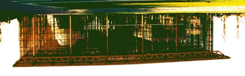
An example of how elegant architecture can be combined with forward looking engine-
ering is offered by the Mont-Cenis Energy Academy at Herne-Sodingen (Fig. 5.1). This
solar-cell clad glass envelope at the site of a former coal mine provides a controlled
Mediterranean microclimate which is powered partly by 1 MWp photovoltaic array and
partly by two co-generation units fuelled by methane released from the disused mine. To
18ensure a good integration into the local electricity supply, the generators are complemen-
ted by a 1.2MWh battery bank. In addition to the Academy, the scheme also export
electricity and heat to 250 units in a nearby housing estate and a local hospital. The Mont-
Cenis Academy is a fine flag-carrier for photovoltaics and new energy engineering –
without a doubt, similar schemes will become more prolific as photovoltaics and energy
efficient solutions become the accepted norm over the next few decades.
Fig. 5.1 The Mont-Cenis Academy at Herne
REFERENCES
P. Baruch, A two-level system as a model for a photovoltaic solar cell, J. Appl. Phys. 57
1347 (1985)
W. Shockley and H.J. Quiesser, Detailed balance limit of efficiency of pn junction solar
cells, J. Appl. Phys, 32, 510 (1961)
R.T. Ross and M. Calvin, Thermodynamics of light emission and free energy storage in
photosynthesis, Biophys. J. 7, 595 (1967)
L.L. Bucciarelli, Estimating loss-of-power probabilities of stand-alone photovoltaic
conversion systems, Solar Energy, 32, 205 (1984); The effect of day-to-day correlation in
solar radiation on the probability of-loss of power in a stand-alone photovoltaic energy
systems, Solar Energy, 36, 11 (1986)
J.P. Gordon, Optimal sizing of stand-alone photovoltaic power systems, Solar Energy 20,
295 (1987)
BIBLIOGRAPHY AND FURTHER READING
M.A. Green, Solar cells: Operating principles, technology and system applications,
Prentice Hall (1981). Other books by Martin Green give a more detailed account of the
operation and design of crystalline silicon and other modern types of solar cells.
B. Voss, T. Knobloch and A. Goetzberger, Crystalline silicon solar cells, Wiley,
Chichester (1998).
T. Markvart (editor), Solar Electricity (2nd edition), Wiley, Chichester (2000).
M.D. Archer and R. Hill (editors), Clean electricity from photovoltaics, Imperial College
Press (2000).
F. Lasnier and T.G. Ang, Photovoltaic Engineering Handbook, Adam Hilger, Bristol,
(1990).
19You can also read