Calculating canopy stomatal conductance from eddy covariance measurements, in light of the energy budget closure problem
←
→
Page content transcription
If your browser does not render page correctly, please read the page content below
Biogeosciences, 18, 13–24, 2021
https://doi.org/10.5194/bg-18-13-2021
© Author(s) 2021. This work is distributed under
the Creative Commons Attribution 4.0 License.

Calculating canopy stomatal conductance from eddy covariance
measurements, in light of the energy budget closure problem
Richard Wehr and Scott R. Saleska
Ecology and Evolutionary Biology, University of Arizona, Tucson, 85721, USA

Correspondence: Richard Wehr (rawehr@email.arizona.edu)

Received: 1 May 2020 – Discussion started: 13 May 2020
Revised: 14 October 2020 – Accepted: 10 November 2020 – Published: 4 January 2021

Abstract. Canopy stomatal conductance is commonly esti-           acterized by the canopy stomatal conductance to water vapor
mated from eddy covariance measurements of the latent heat        (gsV ), which can be defined as the total canopy transpiration
flux (LE) by inverting the Penman–Monteith equation. That         divided by the transpiration-weighted average water vapor
method ignores eddy covariance measurements of the sensi-         gradient across the many real stomata. This canopy stomatal
ble heat flux (H ) and instead calculates H implicitly as the     conductance is not a simple sum of the individual leaf-level
residual of all other terms in the site energy budget. Here       conductances and does not vary with time or environment in
we show that canopy stomatal conductance is more accu-            quite the same way as they do (Baldocchi et al., 1991); it is
rately calculated from eddy covariance (EC) measurements          impacted, for example, by changes in the distribution of light
of both H and LE using the flux–gradient equations that de-       within the canopy.
fine conductance and underlie the Penman–Monteith equa-              When the aerodynamic conductance to water vapor out-
tion, especially when the site energy budget fails to close due   side the leaf (gaV ) is greater than gsV , the latter exerts a strong
to pervasive biases in the eddy fluxes and/or the available en-   influence on transpiration, from which it can be inferred. The
ergy. The flux–gradient formulation dispenses with unneces-       standard method is to calculate gsV from eddy covariance
sary assumptions, is conceptually simpler, and is as or more      (EC) measurements of the latent heat flux (LE) via the in-
accurate in all plausible scenarios. The inverted Penman–         verted Penman–Monteith (iPM) equation (Monteith, 1965;
Monteith equation, on the other hand, contributes substantial     Grace et al., 1995) – but the EC method and the iPM equation
biases and erroneous spatial and temporal patterns to canopy      make a strange pairing. The original (not inverted) Penman–
stomatal conductance, skewing its relationships with drivers      Monteith equation was designed to estimate transpiration
such as light and vapor pressure deficit.                         from the available energy (A), the vapor pressure deficit, and
                                                                  the stomatal and aerodynamic conductances. It was derived
                                                                  from simple flux–gradient relationships for LE and for the
                                                                  sensible heat flux (H ) but was formulated in terms of A and
1   Introduction                                                  LE rather than H and LE. Thus the inverted PM equation
                                                                  estimates gsV from A and LE rather than from H and LE.
Leaf stomata are a key coupling between the terrestrial car-      EC sites, in contrast, measure H and LE but rarely assess A
bon and water cycles. They are a gateway for carbon dioxide       in its entirety. True A is net radiation (Rn ) minus heat flux to
and transpired water and often limit both at the ecosystem        the deep soil (G), minus heat storage (S) in the shallow soil,
scale (Jarvis and McNaughton, 1986). Although the many            canopy air, and biomass. In wetland ecosystems, heat flux by
stomata in a plant canopy experience a wide range of micro-       groundwater discharge (W ) can also be important (Reed et
environmental conditions and therefore exhibit a wide range       al., 2018). While net radiation measurements are ubiquitous
of behaviors at any given moment in time, it has proven use-      at EC sites, ground heat flux measurements are less common
ful in many contexts to approximate the canopy as a sin-          (Stoy et al., 2013; Purdy et al., 2016) and heat storage and
gle “big leaf” with a single stoma (Baldocchi et al., 1991;       discharge measurements are rare (Lindroth et al., 2010; Reed
Wohlfahrt et al., 2009; Wehr et al., 2017). That stoma is char-

Published by Copernicus Publications on behalf of the European Geosciences Union.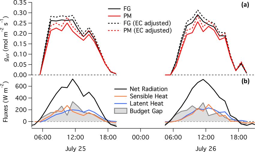
14                                                    R. Wehr and S. R. Saleska: Calculating canopy stomatal conductance

et al., 2018). As such it is common practice to simply omit S     in a more general context (Twine et al., 2000). All but one of
and W and sometimes G from A in the iPM equation.                 the schemes in Wohlfahrt et al. (2009) involve attributing the
   In general, neither S nor G is negligible. Insufficient mea-   half-hourly budget gap entirely to A or entirely to H + LE,
surement of S in particular has been shown (Lindroth et al.,      neither of which is generally realistic according to the subse-
2010; Leuning et al., 2012) to be a major contributor to the      quent results of Leuning et al. (2012), mentioned above. The
infamous energy budget closure problem at EC sites, which         remaining option from Wohlfahrt et al. (2009) increases H
is that the measured turbulent heat flux H +LE is about 20 %      and LE to close the long-term (e.g., daily or monthly) bud-
less than the measured available energy Rn − G on average         get gap while preserving the Bowen ratio (B), which is in line
across the FLUXNET EC site network (Wilson et al., 2002;          with Leuning et al. (2012) in that it attributes the long-term
Foken, 2008; Franssen et al., 2010; Leuning et al., 2012; Stoy    gap to EC and the remaining gap to storage.
et al., 2013). The other major contributor, which also impacts       Here we use data simulations to show that regardless of
the iPM equation, is systematic underestimation of H + LE         whether the energy budget gap is due to A or H + LE, and
by the EC method, probably due to its failure to capture sub-     regardless of how the EC bias is partitioned between the
mesoscale transport (Foken, 2008; Stoy et al., 2013; Charu-       buoyancy flux and Bowen ratio limits, stomatal conductance
chittipan et al., 2014; Gatzsche et al., 2018; Mauder et al.,     is more accurately obtained by direct application of the two
2020). Leuning et al. (2012) assessed the relative contribu-      simple flux–gradient (FG) equations on which the iPM equa-
tions of S and H + LE to the closure problem using the fact       tion is based than by use of the iPM equation itself. By using
that S largely averages out over 24 h while Rn , H , and LE do    simulations, we can know the “true” target values and hence
not; thus S contributes to the hourly but not the daily energy    the absolute biases in gsV . We also use our simulations to
budget (Lindroth et al., 2010; Leuning et al., 2012). Analyz-     test the effects of perfect and imperfect eddy flux corrections
ing over 400 site years of data, they found that the median       and of bias in the aerodynamic conductance outside the leaf.
slope of H + LE versus Rn − G was only 0.75 when plotting         Lastly, we leave the simulations behind and show how the
hourly averages but went up to 0.9 when plotting daily av-        discrepancy between the FG and iPM formulations impacts
erages. This result suggests that for the average FLUXNET         the retrieval of gsV over time using real measurements from
site, 60 % of the energy budget gap is attributable to S and      a conifer forest. We present the FG and iPM formulations in
40 % to H +LE. Depending on the depth at which G is mea-          Sect. 2, describe our methods for comparing them in Sect. 3,
sured (which is not standard), G might also average down          and report our findings in Sect. 4.
considerably over 24 h and thereby share some of the 60 %
attributed to S. Conversely, the part of G that does not aver-
age out over 24 h might share some of the 40 % attributed to      2   Theory
H + LE, as might Rn and W . Part of that 40 % might also be
due to mismatch between the view of the net radiometer and        By definition, conductance is the proportionality coefficient
the flux footprint of the eddy covariance tower. But S and        between a flux and its driving gradient. In the case of gsV ,
H + LE are the most likely sources of large systematic bias       the flux is transpiration and the gradient is the vapor pressure
across sites.                                                     differential across the “big-leaf” stoma. It is therefore rela-
   The iPM equation is further impacted by how the underes-       tively straightforward to calculate gsV from the flux–gradient
timation of H +LE is partitioned between H and LE. While          (FG) equations for transpiration and sensible heat (Baldoc-
some studies have reported that underestimation of H + LE         chi et al., 1991), rearranged as follows (Wehr and Saleska,
roughly preserves the Bowen ratio (B = H /LE), others have        2015):
reported that the failure to capture sub-mesoscale transport
causes EC to underestimate H more than LE (Mauder et                   es (TL ) − ea
                                                                  rsV =              − raV ,                                  (1)
al., 2020) – a situation that would benefit the iPM equation.              RTa E
Charuchittipan et al. (2014) quantified the preferential under-        H raH
                                                                  TL =        + Ta ,                                          (2)
estimation of H relative to LE using a simple formula based            ρa cp
on the buoyancy flux, and a study of tall vegetation sug-
gested that the formula holds when B is high (B>2) but that       where rsV (s m−1 ) is the stomatal resistance to water vapor,
B is instead preserved when it is low or moderate (B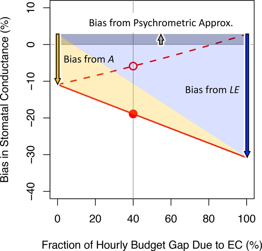
R. Wehr and S. R. Saleska: Calculating canopy stomatal conductance                                                               15

(8.314472 J mol−1 K−1 ). The equation for the saturation va-      where LEtr is the latent heat flux associated with transpira-
por pressure (Pa) as a function of temperature (K) is (World      tion (W m−2 ), LEev is the latent heat flux associated with
Meteorological Organization, 2008)                                evaporation that does not pass through the stomata (W m−2 ),
                                                                es (Ta ) is the saturation vapor pressure of the air as a function
                        17.62(T −273.15)
es (T ) = 611.2e       243.12+(T −273.15)
                                                .          (3)    of Ta (Pa) rather than TL , s is the slope of the es curve at Ta
                                                                  (Pa K−1 ), and γ is the psychrometric constant at Ta (Pa K−1 ).
The aerodynamic resistances describe the path between the         Rn , G, S, and W also have units of watts per square meter.
surface of the big leaf and whatever reference point in the       Latent heat flux is water vapor flux (E) times the latent heat
air at which Ta , ea , ρa , and cp are measured. If that refer-   of vaporization of water (about 44.1 × 10³ J mol−1 ).
ence point is the top of an eddy flux tower, then that path           The inverted PM equation is usually expressed in a slightly
includes the leaf boundary layer (through which transport         simpler form by neglecting the distinctions (a) between tran-
is quasi-diffusive) as well as the canopy airspace and some       spiration and evaporation and (b) between the leaf boundary
above-canopy air (through which transport is turbulent). The      layer resistances to heat and water vapor. We retain those dis-
turbulent eddy resistance (re ) may be calculated by various      tinctions here in order to highlight two important points.
methods that do not agree particularly well with one another
(e.g., see Baldocchi et al., 1991; Grace et al., 1995; Wehr         1. Absent a means to accurately partition the measured
and Saleska, 2015) but is typically small in “rough surface”           eddy flux of water vapor into transpiration and non-
ecosystems like forests during the daytime, when raH and raV           stomatal evaporation (e.g., from soil or wet leaves), the
tend to be dominated by the leaf boundary layer resistances            FG and iPM equations are applicable only when evap-
rbH and rbV . An empirical model such as the one given in the          oration is negligible, which is a difficult situation to
Appendix can be used to calculate rbH as a function of wind            verify but does occur at particular times in particular
speed and other variables. Using that model in a temperate             ecosystems (see, e.g., Wehr et al., 2017).
deciduous forest, rbH was found to vary only between 8 and
12 s m−1 (Wehr and Saleska, 2015), and so we simply take            2. Setting rbV = rbH instead of using Eq. (4) is a good
it to be constant at 10 s m−1 here. The corresponding resis-           approximation for amphistomatous leaves (stomata on
tance to water vapor transport can be calculated from rbH via          both sides) but a poor approximation for the more com-
(Hicks et al., 1987)                                                   mon hypostomatous leaves (stomata on only one side)
               2                                                     (Schymanski and Or, 2017). Indeed, we find that if rbV
        1      Sc 3                                                    is set equal to rbH for hypostomatous leaves, the iPM
rbV =     rbH       ,                                      (4)
        f      Pr                                                      equation underestimates gsV by about 10 % (depending
                                                                       on the relative resistances of the stomata and boundary
where Sc is the Schmidt number for water vapor (0.67), P r             layer) even when the site energy budget is closed.
is the Prandtl number for air (0.71), and f is the fraction
of the leaf surface area that contains stomata (f = 0.5 for          Note that the iPM equation can be derived from the FG
hypostomatous leaves, which have stomata on only one side,        equations by invoking energy balance to replace H with A −
and f = 1 for amphistomatous leaves, which have stomata           LE in Eq. (2) and then linearizing the Clausius–Clapeyron
on both sides). The aerodynamic resistances to sensible heat      relation to eliminate leaf temperature:
and water vapor are then raH = rbH + re and raV = rbV + re .
   Finally, the stomatal conductance to water vapor                  es (Ta ) − es (TL )
(mol m−2 s−1 ) is obtained from rsV by (Grace et al., 1995):      s≈                     ⇒ es (TL ) ≈ es (Ta ) − s (Ta − TL )
                                                                          Ta − TL


           P

                 1                                                                  (A − LE) raH
gsV =              ,                                      (5)      = es (Ta ) + s                    .                          (7)
         RTL rsV                                                                         ρa cp

where P is the atmospheric pressure.                              This psychrometric approximation has been shown to cause
   The above FG theory is also the basis of the Penman–           significant bias and incorrect limiting behavior in the
Monteith equation for a leaf (Monteith, 1965) and its inverted    Penman–Monteith equation (McColl, 2020). McColl (2020)
form (Grace et al., 1995), which can be expressed as              derived a similar, alternative equation that remedies those
                                                                  problems but still uses measurements of A instead of H . The
rsV =                                                             psychrometric approximation and the substitution for H are
s (Rn − G − S − W − LEtr − LEev ) raH + ρa cp (es (Ta ) − ea )    the only two differences between the FG and iPM formula-
                                                                  tions. Both formulations rely on the same water flux mea-
                        γ LEtr
                                                                  surements to estimate transpiration, both approximate the
− raV ,                                                           canopy as a big leaf, and both use the same estimate of aero-
                                                           (6)    dynamic resistance.

https://doi.org/10.5194/bg-18-13-2021                                                          Biogeosciences, 18, 13–24, 2021
16 R. Wehr and S. R. Saleska: Calculating canopy stomatal conductance
3 Methods FLUXNET average). The simulations were explored along
three main axes of variation.
Our analysis consisted of two parts: simulations and real data
analysis. The simulations were designed to unambiguously Variation 1. The energy budget gap was variously ap-
demonstrate the impact of flux measurement biases and the portioned between measurement bias in A and measure-
resultant energy budget gap on FG and iPM calculations of ment bias in H +LE. The measurement bias in H +LE
gsV , as well as to test the sensitivity of gsV to bias in the was applied proportionally to H and LE so as to pre-
estimated aerodynamic resistance outside the leaf; they are serve the true Bowen ratio. All other variables were un-
described in Sect. 3.1. The real data analysis was designed to biased.
assess the magnitude and temporal variation in the discrep-
ancy between the FG and iPM formulations in a real forest Variation 2. Measurements of H and LE biased the
and is described in Sect. 3.2. Bowen ratio by varying amounts while the apportioning
of the energy budget gap between A and H + LE was
3.1 Simulations fixed at the FLUXNET average (60 % A, 40 % H +LE).
All other variables were unbiased.
We assessed the proportional bias in gsV calculated via the
Variation 3. Estimates of the aerodynamic conductance
iPM and FG formulations by simulating observations and
outside the leaf were biased by varying amounts while
using them to estimate gsV . The simulations were of three
the apportioning of the energy budget gap between A
snapshots in time roughly typical of midday in three differ-
and H +LE was fixed at the FLUXNET average and the
ent ecosystems: a temperate deciduous forest in July (the
measurements of H and LE preserved the true Bowen
Harvard Forest in Massachusetts, USA; Wehr et al., 2017),
ratio. All other variables were unbiased.
a tropical rainforest in May (the Reserva Jaru in Rondô-
nia, Brazil; Grace et al., 1995), and a tropical savannah in For each measurement bias scenario, we used the FG and
September (Virginia Park in Queensland, Australia; Leuning iPM formulations to calculate gsV from the simulated (usu-
et al., 2005). The purpose of including three different ecosys- ally erroneous) eddy flux measurements, from perfectly cor-
tems was to test the FG and iPM formulations across a broad rected eddy flux measurements, and from eddy flux measure-
range of environmental and biological input variables (espe- ments adjusted to close the long-term energy budget while
cially Bowen ratios), not to provide a lookup table of quanti- preserving the Bowen ratio, as proposed in Wohlfahrt et
tative gsV corrections for other sites. The particular sites and al. (2009). In our simulations of a single point in time, the
time periods within each ecosystem were chosen merely for latter adjustment was represented by increasing H and LE
convenience, as the requisite variables were readily obtain- proportionally such that H + LE became equal to the true
able from the literature or from our past work. value of A. Such an adjustment restores the true eddy fluxes
The simulations began by setting the “true” target val- if their measurements did not bias the Bowen ratio and was
ues of all the variables involved; in other words, their val- therefore redundant with the perfect correction for Variation
ues without any simulated measurement error. To keep these 1 and Variation 3. Conversely, the perfect correction was of
values realistic, we started with approximate observed fluxes no interest for Variation 2, as it removes all bias in the Bowen
and conditions obtained from the papers cited above or from ratio.
our own work at the Harvard Forest (Table 1), with the pre-
cise values of H and LE chosen to satisfy B and energy 3.2 Analysis of real measured time series
balance. These fluxes and conditions were then used to cal-
culated the true target gsV using the FG equations (Eqs. 1–5). In order to show how the FG and iPM methods differ in a
As the fluxes in Table 1 close the energy budget perfectly, the real forest over the diurnal cycle, we calculated time series
FG and iPM equations are interchangeable for this step of of gsV from real hourly measurements at Howland Forest
the simulations apart from the psychrometric approximation recorded in the AmeriFlux EC site database (Site US-Ho1;
(Eq. 7), which causes a small but significant (∼ 5 %) positive Hollinger, 1996). Howland Forest is a mostly coniferous for-
bias in iPM-derived gsV . That bias is the reason why iPM- est in Maine, USA (45◦ 120 N, 68◦ 440 W), which we chose
derived gsV does not quite converge on the true value even for its intermediate Bowen ratio, for variety, and otherwise
when the entire energy budget gap is due to the EC fluxes for convenience. In addition to using the original measured
and those fluxes are perfectly corrected (see Fig. 2). Thus we fluxes, we also calculated gsV after adjusting the eddy fluxes
could have instead used the iPM equation (Eq. 6) to set the using the long-term energy budget closure scheme proposed
true gsV and obtained similar results, except that the psychro- by Wohlfahrt et al. (2009) – the same flux adjustment scheme
metric approximation bias would have appeared, incorrectly, we tested in our simulations. For this scheme at Howland
to afflict the FG results instead of the iPM results. Forest, we computed the slope of H + LE versus Rn − G
Next, we simulated a wide range of measurement bias from a plot of all 24 h averages in the summer of 2014 and
scenarios, each with a 20 % gap in the energy budget (the then divided both H and LE by that slope.
Biogeosciences, 18, 13–24, 2021 https://doi.org/10.5194/bg-18-13-2021R. Wehr and S. R. Saleska: Calculating canopy stomatal conductance 17
Table 1. Values of environmental and biological variables used in the error simulations (representing midday).
Variable Temperate forest Tropical forest Tropical savannah
(representing July at (representing May at (representing September
the Harvard Forest, USA, Reserva Jaru, Brazil, at Virginia Park,
42◦ 320 N, 72◦ 100 W) 10◦ 50 S, 61◦ 570 W) Australia, 35◦ 390 S, 148◦ 90 E)
Bowen ratio, B 0.6 0.35 8
Sensible heat flux, H (W m−2 ) 236 140 418
Latent heat flux, LE (W m−2 ) 394 400 52
Net radiation, Rn (W m−2 ) 700 600 600
Heat storage, S + G (W m−2 ) 70 60 130
Air temperature, Ta (K) 298 296 303
Atmospheric vapor, ea (Pa) 1700 1800 1800
For all sites, W = 0 W m−2 , rbH = 10 s m−1 , re = 0 s m−1 , P = 101 325 Pa, and f = 0.5.
To minimize the influence of non-stomatal evaporation, mated (as in the FG equations) than to have LE underesti-
we focused on 2 sunny midsummer days more than 24 h af- mated and H overestimated (as in the iPM equation). The
ter the last rain (25–26 July 2014). Because our aim was dashed lines in Fig. 1 show results calculated using eddy
to show the relative bias between the FG and iPM meth- fluxes that have been corrected back to the true values (as
ods rather than to obtain the most accurate possible estimate studies have aimed to do), in which case the FG formulation
of gsV , we used the constant and roughly appropriate values becomes unbiased while the iPM equation still suffers from
rbH = 10 s m−1 and re = 0 as in our simulations, rather than bias in A and from the psychrometric approximation. Fig-
calculating values for these aerodynamic resistances from the ure 2 clarifies the contributions of LE, A, and the psychro-
data according to models like that in the Appendix. Given metric approximation (Eq. 7) to bias in the iPM equation.
that conifer forests are very rough surfaces and that the two Comparison of Fig. 1a, b, and c reveals that the qualitative
daylight periods under consideration were windy with strong relationships in Fig. 1 do not depend on the values of the en-
turbulent mixing (wind speed >3 m s−1 and friction veloc- vironmental and biological variables in Table 1, but the sever-
ity >0.6 m s−1 from late morning through late afternoon), it ity of the bias in gsV does. The bias in gsV is also proportional
is almost certain that the aerodynamic resistance was much to the relative energy budget gap, i.e., (H + LE)/(Rn − G),
less than the stomatal resistance and therefore that the FG and and will therefore be larger (smaller) than shown here at sites
iPM equations were insensitive to rbH and re (see Sect. 4.1). with gaps larger (smaller) than 20 %. Because the bias in gsV
varies with environmental and biological site characteristics,
it will lead to erroneous spatial patterns in gsV and to erro-
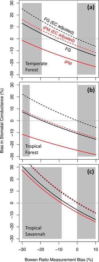
4 Results and discussion neous relationships with potential drivers.
As noted in the introduction, pervasive eddy flux biases
4.1 Absolute biases revealed by simulations likely preserve the true Bowen ratio in some but not all cir-
cumstances. Thus Fig. 3 shows bias in gsV versus bias in the
Our simulations indicate that the flux–gradient formulation measured Bowen ratio. This figure follows Variation 2 from
is substantially more accurate than the inverted Penman– Sect. 3.1, which assumes that 40 % of the energy budget gap
Monteith equation regardless of the cause and magnitude of is due to the eddy fluxes (which is the FLUXNET average).
the energy budget gap and regardless of the ecosystem type. The FG formulation (solid black lines) remains more accu-
Figure 1 shows bias in gsV versus the relative contribution rate than the iPM equation (solid red lines) everywhere be-
of eddy flux bias to the hourly energy budget gap (the re- tween the buoyancy-flux-based and Bowen-ratio-preserving
mainder of the gap being due to bias in the available energy). limits, except very close to the buoyancy-flux-based limit in
This figure follows Variation 1 from Sect. 3.1, which assumes the high-B tropical savannah. The iPM equation becomes
that eddy flux measurements preserve the true Bowen ratio. nearly unbiased in that situation because its inherent assump-
Here the FG formulation (solid black lines) is always more tion that the energy budget gap is due entirely to H becomes
accurate than the iPM formulation (solid red lines) because nearly true; moreover, the small remaining bias due to un-
regardless of whether the gap is due to negative measurement derestimation of LE is offset by bias from the psychromet-
bias in A or in H + LE, the iPM equation implicitly overes- ric approximation, which has the opposite sign (see Fig. 2).
timates H (as the residual of the other fluxes) and therefore The dotted lines in Fig. 3 show results calculated using eddy
the leaf temperature and therefore the water vapor gradient, fluxes that have been adjusted to close the long-term energy
which exacerbates underestimation of the conductance. In budget while preserving the (erroneously measured) Bowen
other words, it is better to have both LE and H underesti-
https://doi.org/10.5194/bg-18-13-2021 Biogeosciences, 18, 13–24, 202118 R. Wehr and S. R. Saleska: Calculating canopy stomatal conductance
Figure 2. Inverted Penman–Monteith results from Fig. 1a, anno-
tated to indicate the various sources of bias.
to favor the iPM equation as that bias increases – and it illus-
trates how improper correction of the eddy fluxes can make
the bias in gsV worse.
Aside from the energy budget gap, another potentially im-
portant source of bias in the FG and iPM equations is the
aerodynamic resistance (raH = rbH + re and raV = rbV + re ).
Estimates of the aerodynamic resistance come from models
of the leaf boundary layer (such as that in the Appendix)
and of micrometeorology (see Baldocchi et al., 1991). These
models are based on established theory and careful exper-
iments but involve many parameters and assumptions that
are not well constrained in real ecosystems. As a result, the
uncertainty in the aerodynamic resistance is generally un-
known. Figure 4 shows how bias in gsV is impacted by a
range of plausible biases in the estimated boundary layer re-
sistance (a factor of 2 in either direction), following Variation
3 from Sect. 3.1. Here the apportioning of the energy budget
gap between A and H + LE is fixed at the FLUXNET av-
Figure 1. Proportional bias in canopy stomatal conductance ob- erage and the measurements of H and LE preserve the true
tained from the flux–gradient (FG, black) and inverted Penman– Bowen ratio. Especially when the Bowen ratio is far from 1
Monteith (iPM, red) formulations versus the fraction of the hourly (Fig. 4b, c), plausible bias in the boundary layer estimate can
energy budget gap caused by bias in the eddy fluxes rather than by lead to large biases in gsV regardless of whether the FG or
bias in the available energy. Solid lines show results without eddy iPM formulation is used. On the other hand, when B = 0.6
flux correction and dashed lines show results with perfectly cor- in the temperate forest (Fig. 4a), the effects of the boundary
rected eddy fluxes. The average estimated contribution of eddy flux layer on sensible and latent heat roughly cancel one another
bias to the budget gap across FLUXNET is indicated by the grey out in the FG formulation, so that gsV is insensitive to the
vertical line (Leuning et al., 2012). Circles highlight where the var- boundary layer estimate. Biases in the boundary layer resis-
ious lines cross the FLUXNET average.
tance rarely make the iPM equation more accurate than the
FG equations.
If the aerodynamic resistance outweighs the stomatal re-
ratio (if the eddy fluxes were perfectly corrected as in Fig. 1, sistance, then transpiration is insensitive to the stomata and
there would be no variation along the abscissa for any method it is inadvisable to try to retrieve gsV from measurements
in this figure). We include this mis-correction because it is of the water vapor flux. Essentially, transpiration does not
the most likely adjustment to be applied to eddy fluxes in carry much information about the stomata in this case, and
practice, whether it is appropriate or not. It favors the FG so the uncertainty in retrieved gsV would be large regard-
formulation when the Bowen ratio bias is small and begins less of whether the FG or iPM formulation was used. This is
Biogeosciences, 18, 13–24, 2021 https://doi.org/10.5194/bg-18-13-2021R. Wehr and S. R. Saleska: Calculating canopy stomatal conductance 19
Figure 3. Proportional bias in canopy stomatal conductance ob- Figure 4. Proportional bias in canopy stomatal conductance ob-
tained from the flux–gradient (FG, black) and inverted Penman– tained from the flux–gradient (FG, black) and inverted Penman–
Monteith (iPM, red) formulations versus proportional bias in the Monteith (iPM, red) formulations versus proportional bias in the es-
measured Bowen ratio. Solid lines show results without eddy flux timated boundary layer resistance. Solid lines show results without
correction, and dotted lines show results with the eddy fluxes ad- eddy flux correction, and dashed lines show results with perfectly
justed to close the long-term energy budget while preserving the corrected eddy fluxes.
(erroneously measured) Bowen ratio. The unshaded region denotes
the plausible range of pervasive bias, which is bounded by the
buoyancy-flux-based and Bowen-ratio-preserving limits (see text).
(rbH bias = 0, marked by the vertical grey line), then the
FG equations actually become slightly more accurate in this
the “decoupled” limit described by Jarvis and McNaughton limit while the iPM equation becomes substantially more bi-
(1986) and the “calm limit” described by McColl (2020). ased. The reason is that a large aerodynamic resistance im-
Comparison of Fig. 5 to Fig. 4a demonstrates that as the pedes the exchange of heat and so increases the leaf temper-
ecosystem moves toward this limit, the sensitivity of gsV ature, which increases the saturation vapor pressure inside
to bias in the aerodynamic resistance increases as expected; the leaf by an even greater factor (according to the nonlinear
however, if the aerodynamic resistance is estimated perfectly Clausius–Clapeyron relation). Thus transpiration actually in-
https://doi.org/10.5194/bg-18-13-2021 Biogeosciences, 18, 13–24, 202120 R. Wehr and S. R. Saleska: Calculating canopy stomatal conductance
Figure 6. (a) Hourly canopy stomatal conductance to water vapor
calculated at Howland Forest (Hollinger, 1996) over 2 d in 2014 by
Figure 5. Same as Fig. 4a, but with true boundary layer resistance the same approaches as in Fig. 3. (b) Measured energy fluxes and
increased to make the aerodynamic and stomatal conductances to budget gap.
water vapor equal, simulating very calm atmospheric conditions and
increasing the sensitivity of the FG and iPM equations to the value
used for the boundary layer resistance. tion in the late afternoon. The diurnal curve obtained from
the iPM equation is therefore too flat, leading to an under-
stated picture of the response of gsV to the vapor pressure
creases and the Bowen ratio approaches zero, so that under- deficit (which peaks in the afternoon), and/or to an exagger-
estimation of H becomes unimportant but underestimation ated picture of the saturation of gsV at high light. This time-
of LE becomes more important. The psychrometric approx- varying discrepancy between the FG and iPM approaches
imation also becomes poorer in this situation because it is can be explained by the fact that S (and therefore negative
a linearization of the Clausius–Clapeyron relation (McColl, bias in the iPM equation) generally peaks in the late morning
2020). and approaches zero in the late afternoon (Grace et al., 1995;
Lindroth et al., 2010), as reflected in the energy budget gap
4.2 Relative biases over time in a real forest shown in the bottom panel of Fig. 6 (grey shading).
Figure 6 compares the diurnal patterns of gsV calculated from
real measurements at Howland Forest (Hollinger, 1996) us- 5 Conclusions
ing the FG (black) and iPM (red) formulations. Solid lines
show results based on the original EC fluxes and dotted We have shown that for the purpose of determining canopy
lines show results based on adjusted EC fluxes that closed stomatal conductance at eddy covariance sites, the inverted
the long-term energy budget while preserving the measured Penman–Monteith equation is an inaccurate and unnecessary
Bowen ratio (the same adjustment as shown in Fig. 3). As approximation to the flux–gradient equations for sensible
usual at EC sites, heat storage was not measured and was heat and water vapor. Incomplete measurement of the energy
therefore omitted from the iPM equation. If the bias in A did budget at EC sites causes substantial bias and misleading
indeed average out at the monthly timescale, and if the mea- spatial and temporal patterns in canopy stomatal conductance
sured Bowen ratio and estimated aerodynamic resistances derived via the iPM equation, even after attempted eddy flux
were accurate, then the true values of gsV in Fig. 6 should corrections. The biases in iPM stomatal conductance vary be-
be those obtained using the FG formulation with adjusted tween 0 % and ∼ 30 % depending on the time of day and
EC fluxes (dotted black lines). That flux adjustment was rel- the site characteristics, resulting in erroneous relationships
atively small at this site in the summer of 2014: the slope of between stomatal conductance and driving variables such as
hourly H + LE versus hourly Rn − G was only 0.63, while light and vapor pressure deficit. Models trained on those re-
the slope using daily data was 0.92, suggesting that 78 % of lationships can be expected to misrepresent canopy carbon–
the hourly energy budget gap was due to the omission of S water dynamics and to make incorrect predictions.
and only 22 % was due to EC. Besides the expected nega- In theory, the FG equations are mathematically equivalent
tive bias in the iPM approach, Fig. 6 shows that the iPM and to the iPM equation aside from the relatively minor psychro-
FG formulations claim noticeably different diurnal patterns metric approximation in the latter. In practice, however, er-
for gsV . In particular, the iPM equation gives substantially rors in H and LE push gsV in opposite directions and so it
lower values than the FG formulation through the morning is crucial that the FG equations receive underestimates of H
and early afternoon but then converges on the FG formula- and LE whereas the iPM equation implicitly overestimates
Biogeosciences, 18, 13–24, 2021 https://doi.org/10.5194/bg-18-13-2021R. Wehr and S. R. Saleska: Calculating canopy stomatal conductance 21 H = A − LE from overestimates of A (= Rn − G − S − W ) and underestimates of LE. As a result, bias in gsV tends to be only about half as large in the FG equations as in the iPM equation. Moreover, if the eddy fluxes can be properly corrected, then the FG equations become unbiased while the iPM equation still suffers from bias in A. Unfortunately, there does not appear to be a universally appropriate method for correcting the eddy fluxes at present. When the Bowen ratio is low or moderate in tall vegetation like forests, the published evidence supports increasing H and LE proportionally to close the long-term energy bud- get. However, when the Bowen ratio is high, the evidence suggests that H needs a disproportionally larger correction than LE. In that case, we have shown that a Bowen-ratio- preserving correction can make the bias in gsV worse. Our results suggest that future studies should use the FG equations in place of the iPM equation and that published re- sults based on the iPM equation may need to be revisited. It also motivates further work to determine a general and reli- able framework for correcting the measured fluxes of sensi- ble and latent heat at eddy covariance sites. https://doi.org/10.5194/bg-18-13-2021 Biogeosciences, 18, 13–24, 2021
22                                                      R. Wehr and S. R. Saleska: Calculating canopy stomatal conductance

Appendix A: An empirical formula for the leaf
boundary layer resistance to heat transfer

The canopy flux-weighted leaf boundary layer resistance to
heat transfer from all sides of a leaf or needle (s m−1 ) can be
estimated approximately as (McNaughton and Hurk, 1995;
Wehr and Saleska, 2015)
            s        Z1
      150       L
rbH =                     eα(1−ζ )/2 φ (ζ ) dζ,             (A1)
      LAI       uh
                     0

where LAI is the single-sided leaf area index, L is the charac-
teristic leaf (or needle cluster) dimension (e.g., 0.1 m), uh is
the mean wind speed (m s−1 ) at the canopy top height h (m),
ζ is height normalized by h, φ (ζ ) is the vertical profile of the
heat source (which can be approximated by the   R 1 vertical pro-
file of light absorption) normalized such that 0 φ (ζ ) dζ = 1,
and α is the extinction coefficient for the assumed exponen-
tial wind profile:

u(ζ )
      = eα(ζ −1) ,                                          (A2)
 uh

where α = 4.39 − 3.97e−0.258LAI . The wind speed at the top
of the canopy can be obtained from Eq. (A2) with ζ set to
correspond to the wind measurement height atop the flux
tower.

Biogeosciences, 18, 13–24, 2021                                                       https://doi.org/10.5194/bg-18-13-2021
R. Wehr and S. R. Saleska: Calculating canopy stomatal conductance 23
Code availability. The R code used for the simulations and the Igor Hollinger, D.: AmeriFlux US-Ho1 Howland Forest (main tower),
Pro code used for the Howland Forest data analysis are freely avail- dataset, https://doi.org/10.17190/AMF/1246061, 1996.
able in the Dryad data archive under the digital object identifier Jarvis, P. G. and McNaughton, K. G.: Stomatal Control of Tran-
https://doi.org/10.5061/dryad.h44j0zpgp (Wehr and Saleska, 2020). spiration: Scaling Up from Leaf to Region, Adv. Ecol. Res., 15,
1–49, 1986.
Leuning, R., Cleugh, H. A., Zegelin, S. J., and Hughes, D.: Carbon
Author contributions. RW conceived and designed the study, wrote and water fluxes over a temperate Eucalyptus forest and a tropi-
the software code, performed the simulations, and prepared the cal wet/dry savanna in Australia: measurements and comparison
manuscript with contributions from SRS. with MODIS remote sensing estimates, Agr. Forest Meteorol.,
129, 151–173, 2005.
Leuning, R., van Gorsel, E., Massman, W. J., and Isaac, P. R.: Re-
Competing interests. The authors declare that they have no conflict flections on the surface energy imbalance problem, Agr. Forest
of interest. Meteorol., 156, 65–74, 2012.
Lindroth, A., Mölder, M., and Lagergren, F.: Heat storage in for-
est biomass improves energy balance closure, Biogeosciences, 7,
301–313, https://doi.org/10.5194/bg-7-301-2010, 2010.
Acknowledgements. Funding for AmeriFlux data resources was
Mauder, M., Foken, T., and Cuxart, J.: Surface-Energy-Balance
provided by the U.S. Department of Energy’s Office of Science.
Closure over Land: A Review, Bound.-Lay. Meteorol., 177, 395–
The Howland Forest data were produced under the supervision of
426, https://doi.org/10.1007/s10546-020-00529-6, 2020.
David Hollinger.
McColl, K. A.: Practical and Theoretical Benefits of an Alternative
to the Penman-Monteith Evapotranspiration Equation, Water Re-
sour. Res., 56, 205–215, 2020.
Financial support. This research has been supported by the Na- McNaughton, K. G. and Hurk, B. A.: ‘Lagrangian’ revision of the
tional Science Foundation, Division of Environmental Biology resistors in the two-layer model for calculating the energy budget
(grant no. 1754803). of a plant canopy, Bound.-Lay. Meteorol., 74, 261–288, 1995.
Monteith, J.: Evaporation and environment, Symp. Soc. Exp. Biol.,
19, 205–234, 1965.
Review statement. This paper was edited by Christopher Still and Purdy, A. J., Fisher, J. B., Goulden, M. L., and Famiglietti, J. S.:
reviewed by Bharat Rastogi and one anonymous referee. Ground heat flux: An analytical review of 6 models evaluated at
88 sites and globally, J. Geophys. Res.-Biogeosci., 121, 3045–
3059, 2016.
Reed, D. E., Frank, J. M., Ewers, B. E., and Desai, A. R.: Time
dependency of eddy covariance site energy balance, Agr. Forest
References Meteorol. 249, 467–478, 2018.
Schymanski, S. J. and Or, D.: Leaf-scale experiments reveal an
Baldocchi, D. D., Luxmoore, R. J., and Hatfield, J. L.: Discerning important omission in the Penman–Monteith equation, Hydrol.
the forest from the trees: an essay on scaling canopy stomatal Earth Syst. Sci., 21, 685–706, https://doi.org/10.5194/hess-21-
conductance, Agr. Forest Meteorol., 54, 197–226, 1991. 685-2017, 2017.
Charuchittipan, D., Babel, W., Mauder, M., Leps, J.-P., and Foken, Stoy, P. C., Mauderb, M., Foken, T., Marcolla, B., Boegh, E., Ibrom,
T.: Extension of the Averaging Time in Eddy-Covariance Mea- A., Arain, M. A., Arneth, A., Aurela, M., Bernhofer, C., Cescatti,
surements and Its Effect on the Energy Balance Closure, Bound.- A., Dellwik, E., Duce, P., Gianelle, D., van Gorsel, E., Kiely, G.,
Lay. Meteorol., 152, 303–327, 2014. Knohl, A., Margolis, H., McCaughey, H., Merbold. L., Montag-
Foken, T.: The energy balance closure problem: An overview, Ecol. nani, L., Papale, D., Reichstein, M., Saunders, M., Serrano-Ortiz,
Appl., 18, 1351–1367, 2008. P., Sottocornola, M., Spano D., Vaccari, F., and Varlagin, A.: A
Franssen, H. J. H., Stöckli, R., Lehner, I., Rotenberg, E., and Senevi- data-driven analysis of energy balance closure across FLUXNET
ratne, S. I.: Energy balance closure of eddy-covariance data: A research sites: The role of landscape scale heterogeneity, Agr.
multisite analysis for European FLUXNET stations, Agr. Forest Forest Meteorol., 171–172, 137–152, 2013.
Meteorol., 150, 1553–1567, 2010. Twine, T. E., Kustas, W. P., Norman, J. M., Cook, D. R., Houser, P.
Gatzsche, K., Babel, W., Falge, E., Pyles, R. D., Paw U, K. R., Meyers, T. P., Prueger, J. H., Starks, P. J., and Wesely, M. L.:
T., Raabe, A., and Foken, T.: Footprint-weighted tile ap- Correcting eddy-covariance flux underestimates over a grassland,
proach for a spruce forest and a nearby patchy clearing Agr. Forest Meteorol., 103, 279–300, 2000.
using the ACASA model, Biogeosciences, 15, 2945–2960, Wehr, R. and Saleska, S. R.: An improved isotopic method for par-
https://doi.org/10.5194/bg-15-2945-2018, 2018. titioning net ecosystem–atmosphere CO2 exchange, Agr. Forest
Grace, J., Lloyd, J., and McIntyre, J.: Fluxes of carbon dioxide and Meteorol., 214–215, 515–531, 2015.
water vapour over an undisturbed tropical forest in south-west Wehr, R., Commane, R., Munger, J. W., McManus, J. B., Nelson, D.
Amazonia, Glob. Change Biol., 1, 1–12, 1995. D., Zahniser, M. S., Saleska, S. R., and Wofsy, S. C.: Dynamics
Hicks, B. B., Baldocchi, D. D., Meyers, T. P., Hosker Jr., R. P., and of canopy stomatal conductance, transpiration, and evaporation
Matt, D. R.: A preliminary multiple resistance routine for deriv- in a temperate deciduous forest, validated by carbonyl sulfide up-
ing dry deposition velocities from measured quantities, Water Air
Soil Poll., 36, 311–330, 1987.
https://doi.org/10.5194/bg-18-13-2021 Biogeosciences, 18, 13–24, 202124 R. Wehr and S. R. Saleska: Calculating canopy stomatal conductance take, Biogeosciences, 14, 389–401, https://doi.org/10.5194/bg- Wohlfahrt, G., Haslwanter, A., Hörtnagl, L., Jasoni, R. L., Fenster- 14-389-2017, 2017. maker, L. F., Arnone III, J. A., and Hammerle, A.: On the conse- Wehr, R. and Saleska, S.: Software code for simulations quences of the energy imbalance for calculating surface conduc- and analyses concerning the calculation of canopy stom- tance to water vapour, Agr. Forest Meteorol., 149, 1556–1559, atal conductance at eddy covariance sites, Dryad, Dataset, 2009. https://doi.org/10.5061/dryad.h44j0zpgp, 2020. World Meteorological Organization: Guide to Meteorological In- Wilson, K., Goldstein, A., Falge, E., Aubinet, M., Baldocchi, D., struments and Methods of Observation No. WMO-No. 8, 2008. Berbigier, P., Bernhofer, C., Ceulemans, R., Dolman, H., Field, C., Grelle, A., Ibrom, A., Law, B.E., Kowalski, A., Meyers, T., Moncrieff, J., Monson, R., Oechel, W., Tenhunen, J., Valentini, R., and Verma, S.: Energy balance closure at FLUXNET sites, Agr. Forest Meteorol., 113, 223–243, 2002. Biogeosciences, 18, 13–24, 2021 https://doi.org/10.5194/bg-18-13-2021
You can also read