Vortex precession and exchange in a Bose-Einstein condensate
←
→
Page content transcription
If your browser does not render page correctly, please read the page content below
Published for SISSA by        Springer
                                                                     Received: May 21, 2021
                                                                      Accepted: July 9, 2021
                                                                     Published: July 21, 2021

Vortex precession and exchange in a Bose-Einstein
condensate

                                                                                                JHEP07(2021)157
Julien Garaud,a Jin Daib and Antti J. Niemib,c,d,1
a
  Institut Denis Poisson CNRS-UMR 7013, Université de Tours,
  Tours 37200, France
b
  Nordita, Stockholm University and Uppsala University,
  Roslagstullsbacken 23, SE-106 91 Stockholm, Sweden
c
  Pacific Quantum Center, Far Eastern Federal University,
  690950 Sukhanova 8, Vladivostok, Russia
d
  Department of Physics, Beijing Institute of Technology,
  Haidian District, Beijing 100081, China

    E-mail: garaud.phys@gmail.com, jin.dai@fysik.su.se, Antti.Niemi@su.se

Abstract: Vortices in a Bose-Einstein condensate are modelled as spontaneously symme-
try breaking minimum energy solutions of the time dependent Gross-Pitaevskii equation,
using the method of constrained optimization. In a non-rotating axially symmetric trap,
the core of a single vortex precesses around the trap center and, at the same time, the phase
of its wave function shifts at a constant rate. The precession velocity, the speed of phase
shift, and the distance between the vortex core and the trap center, depend continuously
on the value of the conserved angular momentum that is carried by the entire condensate.
In the case of a symmetric pair of identical vortices, the precession engages an emergent
gauge field in their relative coordinate, with a flux that is equal to the ratio between the
precession and shift velocities.

Keywords: Solitons Monopoles and Instantons, Spontaneous Symmetry Breaking,
Effective Field Theories

ArXiv ePrint: 2010.04549

    1
        Corresponding author.

Open Access, c The Authors.
                                                     https://doi.org/10.1007/JHEP07(2021)157
Article funded by SCOAP3 .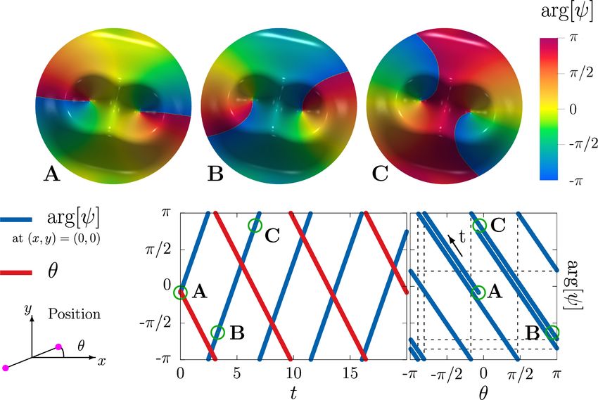
Contents

1 Introduction                                                                            1

2 Theoretical developments                                                                3

3 Numerical simulations                                                                   5

4 Exchange of vortices                                                                    7

                                                                                               JHEP07(2021)157
5 Summary and outlook                                                                     8

A Nondimensionalization of the Gross-Pitaevskii equation                                  9

B Constrained minimization with fixed angular momentum versus
  minimization at constant angular velocity                                              10

C Details of the numerical methods                                                       13
  C.1 Finite-element formulation                                                         13
  C.2 Constrained minimization: Augmented Lagrangian Method                              14
  C.3 Time evolution: forward extrapolated Crank-Nicolson algorithm                      15

1   Introduction

Bose-Einstein condensate is a widely investigated realization of a coherent macroscopic
quantum state. In particular, dilute condensates of trapped ultra-cold atoms have unique
quantum features that facilitate a high level of experimental control [1–3]. Various real-
izations are studied vigorously, both in earth-bound and in earth-orbiting laboratories [4].
Among the goals is the development of ultra-sensitive sensors and detectors [5], and the
properties of cold atom condensates are also employed as a platform for quantum compu-
tation and simulation [6].
     Quantum vortices are the principal topological excitations in a cold atom Bose-Einstein
condensate [7–10]. A vortex is characterized by an integer valued circulation of the macro-
scopic wave function ψ(x)
                                    1
                                       I
                                         d`·∇ arg[ψ] ∈ Z
                                   2π
around its core. The time-dependent Gross-Pitaevskii equation [11, 12] governs the dy-
namics of the macroscopic wave function, at the level of the mean field theory. This is a
nonlinear Schrödinger equation with a quartic nonlinearity that accounts for interactions
between the atoms [13–17].

                                           –1–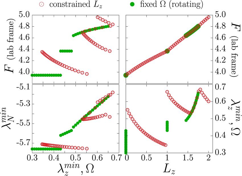
JHEP07(2021)157
Figure 1. Examples of asymmetric vortex configurations of a Bose-Einstein condensate in an axially
symmetric harmonic trap. The elevation of the semitransparent surface stems for the condensate
density |ψ|2 , while the coloring projected onto the xy-plane indicates the value of the phase arg[ψ]
of the macroscopic wave function. The examples shown are minima of the two dimensional Gross-
Pitaevskii free energy (2.2), with non-integer values of the angular momentum (2.3) Lz = 0.80 (left
panel) and Lz = 1.48 (right panel). The vortices precess around the trap center in accordance with
the time dependent Gross-Pitaevskii equation (2.1).

    Vortices that appear in rotating cold atom Bose-Einstein condensates have been ex-
tensively studied, both experimentally and theoretically [16, 18, 19]. At the level of the
Gross-Pitaevskii equation these vortices are commonly modelled as stationary solutions
in a co-rotating frame [13–17, 20–22]. The rotating condensate accommodates growing
angular velocity by forming vortices. This goes with a discontinuous increase in angular
momentum: a rotating condensate does not support an arbitrary value of the angular
momentum [20].
    Here we are interested in solutions of the Gross-Pitaevskii equation in a trapped con-
densate that does not rotate. In that case, the equation has no time independent solutions
besides the trivial one ψ(x) ≡ 0. However, we show that whenever the non-rotating con-
densate supports a non-vanishing arbitrary valued angular momentum, there is a stable
minimum energy solution of the time dependent Gross-Pitaevskii equation. These solu-
tions describe eccentric vortices that precess around the center of the non-rotating axially
symmetric trap, as illustrated in figure 1. In particular, the single vortex solutions are very
similar to the experimentally observed precessing vortices reported in [23].
     It is notable that even though the solutions that we present are minima of the ensuing
free energy, they are not critical points of the free energy. Thus we employ methods of
constrained optimization [24, 25], to solve the time dependent Gross-Pitaevskii equation.
     We note that the microscopic, individual atom angular momentum is certainly quan-
tized. But as pointed out in [26, 27] (see also [20]), in the limit where the number of atoms
is very large, the condensate can accommodate arbitrary values of the macroscopic angular
momentum that appears as a Noether change in the Gross-Pitaevskii equation. It was
pointed out in [26, 27] and confirmed by the variational analysis in [27], in the case of a
single vortex, that a solution with arbitrary angular momentum must in general be time
dependent. Our results confirm this proposal.

                                               –2–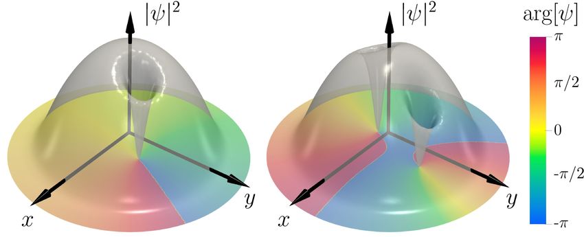
We emphasize the following difference between our approach that considers a non-
rotating trap and builds on the ideas of [26, 27], and the more common approach that
considers vortices in a rotating trap, in terms of a co-rotating frame [13–17, 20–22]: in the
rotating trap problem, the minimal energy state is controlled by the value of the angular
velocity of the trap that appears as a free parameter in the stationary, time independent
co-rotating Gross-Pitaevskii energy functional. The vortices appear as critical points of
this energy functional, as solutions of the time independent Gross-Pitaevskii equation they
minimize an unconstrained variational problem. In contrast, in our case we use the fact
that the angular momentum is conserved, thus we fix its value. The vortices are then solu-
tions to a constrained optimization problem and solve the time dependent Gross-Pitaevskii

                                                                                                JHEP07(2021)157
equation. The difference between these two problems is detailed in appendix B.
     Since the vortex configurations that we find are simultaneously both constrained min-
ima of the Gross-Pitaevskii free energy, and time dependent solutions of the ensuing Hamil-
ton’s equation, they bear a certain resemblance to the concept of a classical Hamiltonian
time crystal [28, 29]. Our approach is modelled on the general theory developed in [30];
see also [31].
     We shall further observe that in the case of a symmetric pair of two identical vortices,
the evolution of the minimal energy vortex states, at specified angular momentum, brings
about an exchange of the vortices. The exchange of identical bodies in two dimensions have
been studied extensively, as it can be used to identify anyons. Anyons are two-dimensional
quasiparticles that are neither fermions nor bosons [32, 33]. The anyon statistics implies
that the exchange of the position of two identical particles results in a change of their
quantum mechanical phase which differs from 0 (the case of bosons) or π (the case of
fermions); for reviews on anyons see e.g. [34, 35]). The anyons, that can play an important
role for quantum computing [36], have recently been observed by electronic interferometry
in quantum Hall effect experiments [37].

2   Theoretical developments

We consider a two dimensional single-component Bose-Einstein condensate on the xy-plane
with an axially symmetric, non-rotating, harmonic trap. This approximates for example
an anisotropic three dimensional trap, resulting in an oblate condensate. Following [14, 38]
we assume that the condensate describes a dilute limit of a large number of atoms, with a
two-body repulsive interaction potential between the atoms. The condensate is described
by a macroscopic wave function ψ(x, t) whose dynamics obeys the (dimensionless) time
dependent Gross-Pitaevskii equation [14, 38]:

                                  1       |x|2               δF
                         i∂t ψ = − ∇2 ψ +      ψ + g|ψ|2 ψ ≡      .                     (2.1)
                                  2        2                 δψ ?

Here g is a dimensionless coupling that accounts for the interactions between the atoms. In
a typical Bose-Einstein condensate there are Na ∼ 104 − 106 ultracold alkali atoms and the
corresponding coupling is typically g ∼ 1–104 ; for discussion of the nondimensionalization,

                                           –3–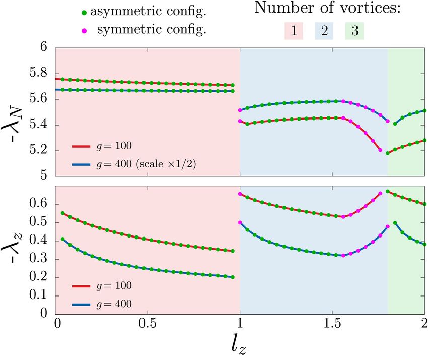
see, e.g, [17] and the appendix A. The free energy F in eq. (2.1) is
                                           (                                )
                                               1         |x|2 2 g 4
                                 Z
                                      2
                           F =       d x         |∇ψ|2 +     |ψ| + |ψ|          .                  (2.2)
                                               2          2       2

     We observe that F is a strictly convex functional, it can not have any critical points
besides the global minimum ψ ≡ 0. Thus there are no nontrivial time independent solutions
of the Gross-Pitaevskii equation (2.1), only time dependent nontrivial solutions of (2.1)
can exist.1 Provided appropriate conditions can be introduced, these solutions can also
minimize the free energy F in the framework of constrained optimization. Thus, we search

                                                                                                            JHEP07(2021)157
for time dependent solutions of (2.1) that are also minima of the free energy (2.2), where
the latter is subject to an appropriate condition.
     Indeed, besides the free energy (2.2) the time evolution equation (2.1) supports two
additional conserved quantities, as Noether charges: the macroscopic angular momentum
along the z-axis                   Z
                                 Lz ≡          d2 x ψ ? ez · (−i~ x ∧ ∇)ψ                          (2.3)

and the norm of the macroscopic wave function a.k.a. the number of particles
                                                    Z
                                               N≡       d2 x ψ ? ψ .                               (2.4)

Accordingly, we search for solutions of the time dependent Gross-Pitaevskii equation (2.1),
with fixed values of both the angular momentum Lz and the number of particles; in the
following, with no loss of generality, we normalize the wave function so that N = 1 (see
appendix A for details). On the other hand, the angular momentum (2.3), can assume
arbitrary values Lz = lz , and even in the case of a single vortex the values lz of the angular
momentum are not expected to be integer valued [26, 27].
     The Lagrange multiplier theorem [39] states that with fixed angular momentum (2.3)
and fixed number of particles (2.4), the minimum of F is also a critical point of

                               Fλ = F + λz (Lz − lz ) + λN (N − 1) .                               (2.5)

Here λz , λN are the Lagrange multipliers that enforce the values Lz = lz and N = 1,
respectively. The critical points (ψcr , λcr   cr
                                          z , λN ) of Fλ (2.5) obey

                      1        |x|2
                     − ∇2 ψ +       ψ + g|ψ|2 ψ = −λN ψ + iλz ez · x ∧ ∇ψ
                      2         2
                            together with Lz = lz and N = 1 .                                      (2.6)

Let ψmin (x) be a solution of (2.6) that is also a minimum of (2.2), and let λmin
                                                                              N and λz
                                                                                        min

denote the corresponding solutions for the Lagrange multipliers. Whenever the solutions
for the Lagrange multipliers do not vanish, ψmin (x) cannot be a critical point of the free
   1
    In the case of a rotating condensate [13–17, 20–22] the angular velocity makes the energy into a non-
convex functional with non-trivial critical points that describe vortices with a discrete valued angular
momentum.

                                                     –4–
energy F in (2.2). Instead, it generates a time dependent solution ψ(x, t) of (2.1) which,
from (2.6), with the initial condition ψ(x, t = 0) = ψmin (x) obeys the linear time evolution
i∂t ψ = −λmin min
N ψ + iλz ez · x ∧ ∇ψ , (2.7)
where both λmin
N and λz
min are time independent [30].
Whenever either of the Lagrange multipliers is non-vanishing, the minimum energy
solution is time dependent. But the time evolution amounts to a simple phase multipli-
cation only when ψmin (x) is an eigenstate of the angular momentum operator; below we
show that this can only occur for lz = 1, for all other values of lz 6= 0 the minimum energy
JHEP07(2021)157
solution always describes a precessing vortex configuration.
The minimum energy wave function ψmin (x) spontaneously breaks both Noether sym-
metries. The time evolution equation (2.7) describes a symmetry transformation of ψmin (x),
that is generated by a definite linear combination of the two conserved Noether charges:
δN δLz
i∂t ψ = −λmin
N − λmin
z ≡ −λmin min
N {N, ψ} − λz {Lz , ψ} , (2.8)
δψ ? δψ ?
where { , } is the Poisson bracket. This is an example of spontaneous symmetry breaking,
but now the symmetry breaking minimum energy configuration is time dependent [30].
3 Numerical simulations
To search for minimum energy solutions of the time dependent Gross-Pitaevskii equation,
we numerically minimize the free energy (2.2) subject to the conditions Lz = lz and N = 1.
The problem is discretized within a finite-element framework [40], and the constrained
optimization problem is then solved using the Augmented Lagrangian Method (see details
of the numerical methods in appendix C). Minimal energy states for angular momentum
values lz ∈ (0, 2] with N = 1, and for three representative values of the interaction coupling
g = 5, g = 100 and g = 400 are displayed in figure 2; see also additional animations in
supplementary materials attached to this paper.
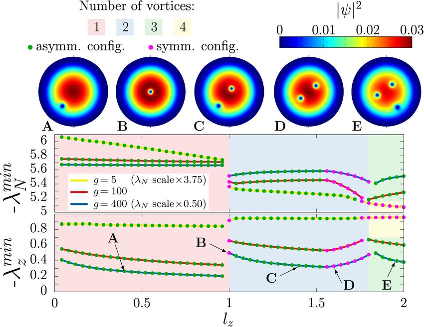
For non-vanishing values of the angular momentum 0 < lz < 1 the minimum energy
configuration ψmin (x) is an eccentric vortex that precesses around the trap center (see
regime A). As lz increases the vortex core approaches the trap center. This kind of
eccentric precessing vortices have been previously proposed theoretically in [27]. They
appear very similar to the precessing vortices that have been observed experimentally [23].
As shown in regime B, when lz = 1, the core position coincides with the center of
the trap, and the Lagrange multipliers feature a discontinuity. At this value of lz , our
solution coincides with the single vortex solution that has been described extensively in
the literature [13–17, 21, 22]. When lz becomes larger than one, a second vortex appears,
and there are two qualitatively different two-vortex configurations. As lz increases, these
are sequentially asymmetric (regime C) and then symmetric (regime D) with respect to
the trap center. Because it depends on g, there is no universal value of lz that separates
these two regimes. At higher values of angular momentum, lz ≈ 1.8 with the exact value
depending on g, additional vortices start entering the condensate; this is the regime E in
–5–JHEP07(2021)157
Figure 2. Minimum energy states for angular momenta lz ∈ (0, 2]. The bottom row shows the
dependence of the multipliers λmin
N and λmin
z on the angular momentum lz for g = 5, 100 and 400.
The panels on the top row display the density of the condensate |ψ|2 for qualitatively different
solutions with g = 400, obtained for different values of lz (zoomed to relevant data while the actual
numerical domain is larger). At the vortex core the density |ψ|2 vanishes and the phase circulation
is 2π. The five regimes A–E are detailed in the text.
figure 2. Remark that for g = 100 and g = 400 a third vortex moves towards the trap
center as lz increases, while for g = 5 a pair of vortices enters. Further increase of the
angular momentum introduces additional vortices in the condensate (not shown).
The case lz = 1, labelled by B in figure 2, is a special case. There, the core of the vortex
coincides with the center of the trap. The corresponding ψmin (x) is an angular momentum
eigenstate with eigenvalue lz = 1, and the solution of the time dependent Gross-Pitaevskii
equation (2.7) is merely an overall phase rotation with no change in the core position.
However, for generic lz the minimum energy configuration ψmin (x) is not an eigenstate of
the angular momentum.
We have simulated the time evolution (2.1) of the minimum energy configuration
ψmin (x) using a Crank-Nicolson algorithm. Simulation details together with animations
of the time evolution can be found in the appendix C. For all values of lz 6= 1 the vortex
configuration precesses uniformly around the trap center. This uniform rotation is a con-
sequence of the equation (2.7) which determines the time evolution of the minimal energy
configurations, in terms of the two conserved charges.
–6–JHEP07(2021)157
Figure 3. The evolution of a minimum energy configuration ψmin (x), in the case of a symmetric
vortex pair (with g = 5) in region D of figure 2. The bottom panels show the evolution of θ, the
rotation angle of the pair, and of the value of the phase arg[ψ] measured at the center of the trap.
The three panels A–C on the top row are snapshots displaying the phase arg[ψ] after rotations
θ = θ0 , θ = θ0 + π and θ = θ0 + 2π respectively. Since the Lagrange multipliers λmin
N and λmin
z are
not commensurate, arg[ψ](t) and θ(t) feature different periodicities. As a result after π rotations
of the pair the phase profile is not simply an overall phase multiplication.
4 Exchange of vortices
Finally, an interesting phenomenon occurs for the time evolution of a symmetric pair of
identical vortices (corresponding to the regime D of figure 2). The time evolution of such
a vortex pair, with g = 5, is displayed in figure 3. The vortex pair rigidly rotates around
the trap center at a constant distance, with an angular velocity specified by λminz ≡ −Ω.
min
In addition the phase of the wave function evolves with a rate that depends on λN . This
coincides with the rate of change in the phase arg[ψ](t), measured at the center of the trap.
Similarly, the rate of change of θ(t) that measures the rotation of the pair, equals λminz .
Since the two Lagrange multipliers are in general not commensurate, it follows that when
the time evolution exchanges the position of two identical vortices, the change in the phase
of the wave function is not by an integer multiple of π.
The quantum mechanical exchange of two identical bodies, with ensuing phase change,
is familiar from description of anyons [32, 33, 41]. The similarity to that scenario can be
elaborated further, by following [41] to rewrite the time evolution (2.7) as follows:
i∂t ψ = Ω Lcov
z ψ ≡ Ω(ez · L + φ ez · x ∧ A)ψ . (4.1)
–7–Here L = −ix ∧ ∇ is the canonical angular momentum, the parameter φ = λmin min
N /λz , and
the flux of A = ∇ tan−1 x/y equals 2π around any counter-clockwise path that encircles
the z-axis once. Notably, in the case of two identical vortices x coincides with their relative
coordinate in a center-of-mass frame. Furthermore, the equation (4.1) is akin a time depen-
dent linear Schrödinger equation that describes the evolution of a charged point particle,
moving on the (x, y) plane under the influence of a unit strength magnetic vortex filament
along the z-axis. The corresponding Hamiltonian comprises the z-component of the co-
variant angular momentum Lcov z . We note that when φ 6= 0, the rotations around z-axis,
i.e. the changes in the polar angle θ, are generated by the covariant angular momentum.
To find the solutions of (4.1) we first remove A by phase multiplication, and then
JHEP07(2021)157
proceed with separation of variables in terms of polar coordinates (r, θ).
Rx
−iφ A·d`
ψ(x, t) = e−iEt X (r, θ) e x0
. (4.2)
The single valuedness of the wave function ψ(x, t) implies that X (r, θ) is generally not
single valued as it obeys
Lz Xn = (n + φ)Xn . (4.3)
The solution of the time evolution (4.1) is thus
Rx
−iφ A·d` X
ψ(x, t) = e x0
fn (r)e−i(n+φ)(Ωt−θ) . (4.4)
n
Here the fn (r) form an orthogonal set of normalizable, real valued functions, they are
selected so that (4.4) describes the energy minimizer ψmin (x) of (2.6), (2.1) at t = 0.
5 Summary and outlook
In summary, we have investigated the time dependent two-dimensional Gross-Pitaevskii
equation, that models dynamics in an axially symmetric harmonic trap. The equation
supports two Noether charges that correspond to the number of atoms and to the ax-
ial component of the macroscopic angular momentum, respectively. We have used the
methodology of constrained optimization to construct solutions that minimize the Gross-
Pitaevskii free energy, with a fixed number of atoms and as function of the macroscopic
angular momentum to which we have assigned arbitrary numerical values. For generic
angular momentum values, a minimum energy configuration always exists and it describes
eccentric vortices that precess uniformly around the center of the trap. In particular, no
time independent solution can exist in a non-rotating cylindrically symmetric trap. More-
over, whenever the solution describes two identical vortices, the time evolution exchanges
their positions but the phase of their common wave function evolves in a nontrivial fashion.
We foresee that the vortex precession in a non-rotating condensate that we have de-
scribed, can be realized and observed in a variety of laboratory experiments; the precessing
vortices already reported in [23] appear to be very similar to the vortex precession that we
–8–have simulated. There are several conceivable experimental setups, where vortices can form
in a non-rotating condensate. These include vortex formation by optical photon beams that
carry a non-vanishing angular momentum, with appropriate topologies [42–45]. Additional
experimental set-ups can be built on thermal quenching in combination with the Kibble-
Zurek mechanism [46–49]. This mechanism describes how topological defects form during
rapid symmetry breaking transitions. There are already several laboratory examples that
are relevant to the scenario we have studied, including neutron irradiation in the case of
superfluid 3 He [50, 51], evaporative cooling in the case of ultracold 8 7Rb atoms [52, 53].
JHEP07(2021)157
Acknowledgments
AJN thanks C. Pethick and K. Sacha for discussions. We thank Rima El Kosseifi for
discussions. The work by DJ and AJN is supported by the Carl Trygger Foundation Grant
CTS 18:276 and by the Swedish Research Council under Contract No. 2018-04411. DJ
and AJN also acknowledge collaboration under COST Action CA17139. The research by
AJN was also partially supported by Grant No. 0657-2020-0015 of the Ministry of Science
and Higher Education of Russia The computations were performed on resources provided
by the Swedish National Infrastructure for Computing (SNIC) at National Supercomputer
Center at Linköping, Sweden.
A Nondimensionalization of the Gross-Pitaevskii equation
In the main body of the paper, the dynamics of a Bose-Einstein ultracold atoms is described
by the dimensionless Gross-Pitaevskii equation. Here, we derive this dimensionless form
from the original equation (see e.g. [17]). In the ultracold dilute regime, the Bose-Einstein
condensate state of Na identical atoms is described by the macroscopic wave function Ψ,
whose dynamics obey
" #
~2 2 Na
i~∂t Ψ = − ∇ + V (x) + g0 |Ψ|2 Ψ , (A.1a)
2m N
4π~2 as
Z
where N = |Ψ|2 , and g0 = . (A.1b)
m
Here, ∇2 ≡ ∇·∇ is the Laplace operator, m is the mass of the atoms, ~ is the reduced
Planck’s constant, and as is s-wave scattering length of the atoms. Note that for practical
purposes, we introduce N to be the norm of the condensate, while Na is the actual number
of atoms in the condensate. The harmonic oscillator trap potential reads as
m 2 2
V (x) = ωx x + ωy2 y 2 + ωz2 z 2 , (A.2)
2
where ωx ≤ ωy ≤ ωz are the trapping frequencies in the different spatial directions. The
dimensionless units are obtained by the following rescaling
s
1 ~
t = ts t̃ , x = xs x̃ , Ψ = x−3/2
s ψ, where ts = , and xs = . (A.3)
ωx mωx
–9–Atoms m (kg) as (m) ωx (rad.s−1 ) Na
87 Rb [1] 1.44 × 10⁻²⁵ 5.1 × 10⁻⁹ 20 102 ∼ 107
23 N a [2] 3.817 × 10⁻²⁶ 2.75 × 10⁻⁹ 2π × 200 ×104 ∼ 5 × 10⁵
4πas
Atoms xs (m) xs g (×N = 1)
87 Rb [1] 6.0 × 10⁻⁶ 1.1 × 10⁻² 1 ∼ 105
23 N a [2] 1.5 × 10⁻⁶ 2.3 × 10⁻² 102 ∼ 104
JHEP07(2021)157
Table 1. Typical physical values for various atomic Bose-Einstein condensates, and the resulting
scale and dimensionless coupling. The reduced Planck constant is ~ = 1.05 × 10⁻³⁴ J.s.
Hence, after dropping the ˜, the dimensionless Gross-Pitaevskii equation is
1
i∂t ψ = − ∇2 + V (x) + g|ψ|2 ψ , (A.4a)
2
1 X ωα 2 2 4πas Na
Z
where V (x) = xα , N = |ψ|2 , and g = . (A.4b)
2 α=x,y,z ωx xs N
The dimensionless time dependent Gross-Pitaevskii equation (A.4), is obtained for a
three dimensional harmonic trap. In the main body of the paper, we consider the case
of a two Bose-Einstein condensate. The two dimensional problem fairly approximates a
disk-shaped condensate with small height in z-direction, for the trap frequencies ωq x ≈ ωy
ωz
and ωz
ωx . This results in a further rescaling of the coupling constant g2d = g3d 2πω x
.
For detailed derivation see, e.g., [17].
The dimensionless coupling g is thus the parameter of the accounts for the interactions
between atoms. In the numerical investigations we choose values g that are representative
of a Bose-Einstein condensate of ultracold alkali atoms. The table 1 shows typical experi-
mental values of trapped ultracold atoms, and the corresponding estimates for the length
scales and the dimensionless coupling g.
B Constrained minimization with fixed angular momentum versus
minimization at constant angular velocity
In the main body of the paper, we emphasize that there is a difference between the common
set-up that describes vortices in a rotating trap in terms of a free energy expressed in the co-
rotating frame [13–17, 20–22], and the present set-up where vortices occur in a non-rotating
trap; the present set-up was first addressed in [26, 27]. Here we clarify the difference, by a
direct comparison of the two cases:
In the case of a rotating trap, vortices are created by rotating the trap, with a constant
angular velocity Ω. The free energy F Ω is expressed in the co-rotating frame, and the
vortices are the critical points of the free energy. The vortex structures can then be
investigated as a function of the externally applied angular velocity Ω. In contrast, in our
case the trap does not rotate. Instead, we use the fact that the angular momentum Lz of
– 10 –the condensate is a conserved quantity, and the condensate carries a corresponding angular
momentum value Lz = lz . The ensuing minimal free energy configuration is a solution
of a constrained optimization problem that minimizes the free energy F , subject to the
condition Lz = lz . The two free energies are related as follows:
Z
F Ω = F − ΩLz , where Lz ≡ d2 x ψ ? ez · (−i~ x ∧ ∇)ψ . (B.1)
Due to the constraint, the free energy minimizer is in general not a critical point of F .
But it can be located using the Lagrange multiplier theorem [39], in the framework of
constrained optimization [24, 25]. Whenever the minimizer of the free energy F is not a
JHEP07(2021)157
critical point, it describes a solution of a time dependent Gross-Pitaevskii equation.
In addition, in both cases the norm of the condensate wave function (i.e. the particle
number) needs to be accounted for. Here the goal is to clarify the difference between
the rotating and non-rotating cases. Therefore, in our comparison we treat the constraint
N = 1 the same way, both when searching for the minimum of F Ω and F , by using
the Lagrange multiplier theorem. For the problem we consider, the Lagrange multiplier
theorem [39] states that with fixed angular momentum and fixed number of particles N ,
the minimum of F is also a critical point of
Fλ ≡ F + λz (Lz − lz ) + λN (N − 1) . (B.2)
Here λz , λN are the Lagrange multipliers that enforce the values Lz = lz and N = 1
respectively. On the other hand, for a rotating condensate, the minimum of F Ω is a critical
point of the following free energy
FλΩ ≡ F Ω + λN (N − 1) = F + ΩLz + λN (N − 1) , (B.3)
where λN is the (only) Lagrange multiplier that enforces N = 1. Note that the present
Lagrange multiplier λN is commonly treated as a chemical potential that is an externally
controlled parameter, in par with Ω. This is not the case here, as λN has to be adjusted
to satisfy the constraint. The critical points of Fλ and FλΩ obey respectively
1 |x|2
Fλ : − ∇2 ψ + ψ + g|ψ|2 ψ = −λN ψ + iλz ez · x ∧ ∇ψ , (B.4a)
2 2
and the conditions Lz = lz and N = 1 ,
1 |x|2
FλΩ : − ∇2 ψ + ψ + g|ψ|2 ψ − iΩ ez · x ∧ ∇ψ = −λN ψ , (B.4b)
2 2
and the condition N = 1 .
Note that in a numerical simulation Ω is an input parameter that is fixed during the
simulation, while λz is adjusted sequentially, to satisfy the constraint (according to the
Augmented Lagrangian Method, see details in section C.2). The differences between the
two approaches are summarized at the end of this section in table 2.
Comparison of the minimal energy solutions of the two equations (B.4), can be seen in
figure 4. The results are indeed quite different. In particular, the free energy (evaluated in
– 11 –Critical Obey the equation Satisfy Control Mult. Output
pts. of Obey the equation params.
|x|2
Fλ − 12 ∇2 ψ + 2 ψ + g|ψ|2 ψ = L z = lz g, lz λN , λmin min
N , λz
−λN ψ + iλz ez · x ∧ ∇ψ and N = 1 λz ψmin
|x|2
FλΩ − 12 ∇2 ψ + 2 ψ + g|ψ|2 ψ N =1 g, Ω λN λmin
N ,
−iΩ ez · x ∧ ∇ψ = −λN ψ ψmin
Table 2. Summary of the differences: the red font shows the parameters that are given as input
to the corresponding minimization problem. The purple font highlights the Lagrange multipliers.
JHEP07(2021)157
In a numerical simulation, these are sequentially adjusted according the Augmented Lagrangian
Algorithm, until the constraints are satisfied (and the minima of Fλ are found). The olive color
fonts show the output quantities obtained in the numerical simulations.
Figure 4. Detailed comparison of the solutions to the two equations (B.4) for g = 100. The panels
on the top row display the energy, in a non-rotating frame, as a function of angular velocity Ω (left)
and value of angular momentum Lz (right). The empty (red) circles denote the results from the
constrained minimization at given value of the angular momentum Lz . The filled (green) circles
show the results from the minimization of a rotated condensate at given angular velocity Ω.
a non-rotating laboratory frame) that is displayed on the panels on the top row of figure 4,
show that the minimization with fixed angular frequency Ω cannot support solutions with
arbitrary values of angular momentum. Indeed, there are excluded ranges
Lz ∈ [0, 1[ ∪ ]1, 1.457[ ∪ ]1.75, 2.68[· · · , (B.5)
where there are no rotation-induced stable vortex states (see the green dots on the top right
panel). This is in agreement with the known results for rotating Bose-Einstein condensates;
– 12 –compare for example the green dots in the top left panel of figure 4, e.g. with the results
shown in figure 2 of [20]. In contrast, in the present case, there cannot be any excluded
values of the angular momentum in the equation (B.4a) (see the red dots on the top right
panel). Those vortex configurations with angular momentum in the excluded ranges (B.5)
describe eccentric asymmetric vortex configurations that precess around the trap center.
Observe that in the case of equation (B.4a), there is multi-valuedness in the free energy
(red dots), as a function of the Lagrange multiplier λz ; see for example the top left panel
at λmin
z ≈ 0.55 which displays 3 different states at the same value of λz . These are a single
eccentric vortex, an asymmetric vortex pair, and a symmetric vortex pair for increasing
JHEP07(2021)157
free energy, respectively. These configurations have both a different angular momentum
value, and a different value of the Lagrange multiplier λmin
N (see the bottom panels) which
plays the role of a chemical potential. The present comparisons, summarized in figure 4,
show that the two equations (B.4a) and (B.4b) do indeed describe two quite different
physical scenarios.
C Details of the numerical methods
In the numerical investigations in the main body of the paper, we use Finite-Element
Methods (FEM) (see e.g. [54, 55]) both for the minimization and for the time-evolution.
In practice we use the finite-element framework provided by the FreeFEM library [40].
Within the finite-element framework, the constrained minimization is addressed using an
Augmented Lagrangian Method together within a non-linear conjugate gradient algorithm.
The time-dependent Gross-Pitaevskii equation, is integrated using a Crank-Nicolson algo-
rithm with a forward extrapolation of the nonlinear term.
C.1 Finite-element formulation
We consider the domain Ω which a bounded open subset of R2 and denote ∂Ω its boundary.
H(Ω) stands for the Hilbert space, such that a function belonging to H(Ω), and its weak
derivatives have a finite L2 -norm. Furthermore, H(Ω) = {u + iv | u, v ∈ H(Ω)} denotes the
Hilbert spaces of complex-valued functions. The Hilbert spaces of real- and complex-valued
functions are equipped with the inner products h·, ·i, defined as:
Z Z
hu, vi = uv , for u, v ∈ H(Ω) , and hu, vi = u? v , for u, v ∈ H(Ω) . (C.1)
Ω Ω
The spatial domain Ω is discretized as a mesh of triangles using for the Delaunay-Voronoi
algorithm, and the regular partition Th of Ω refers to the family of the triangles that
compose the mesh. Given a spatial discretization, the functions are approximated to belong
to a finite-element space whose properties correspond to the details of the Hilbert spaces
(2)
to which the functions belong. We define Ph as the 2-nd order Lagrange finite-element
(2)
subspace of H(Ω), and correspondingly Ph for H(Ω). Now, the physical degrees of freedom
can be discretized in their finite element subspaces. And we define the finite-element
(2)
description of the degrees of freedom as ψ 7→ ψ (h) ∈ Ph . This describes a linear vector
– 13 –space of finite dimension, for which a basis can be found. The canonical basis consists of
the shape functions φk (x), and thus
M
( )
(2)
X (2)
Vh (Th , P )= w(x) = wk φk (x), φk (x) ∈ Ph . (C.2)
k=1
Here M is the dimension of Vh (the number of vertices), the wk are called the degrees of
freedom of w and M the number of the degrees of freedom. To summarize, a given function
is approximated as its decomposition: w(x) = M
P
k=1 wk φk (x), on a given basis of shape
functions φk (x) of the polynomial functions P(2) for the triangle Tik . The finite element
JHEP07(2021)157
space Vh (Th , P(2) ) hence denotes the space of continuous, piecewise quadratic functions of
x, y on each triangle of Th .
C.2 Constrained minimization: Augmented Lagrangian Method
In the main body of the paper, we aim to minimize the free energy while enforcing a set
of two conditions. Such problems, referred to as constrained optimization are studied in
great details, see for example textbooks [24, 25, 56, 57]. Here we describe the numerical
algorithms that were used in the main body of the paper, to solve the constrained optimiza-
tion problem. The Augmented Lagrangian Method (ALM) used to solve the constrained
optimization is based on the following. In terms of the original energy functional to be
minimized F , and the set of conditions Ci , the augmented Lagrangian F aug is defined as
µ X X
F aug := F + Cj2 + λj C j . (C.3)
2 j j
Here µ is a penalty parameter and λj are the Lagrange multipliers associated with the
conditions Cj . In the Augmented Lagrangian Method, the augmented Lagrangian is mini-
mized, and the penalty µ is iteratively increased while the multipliers λj ← λj + µCj until
all conditions are satisfied with a specified accuracy. The ALM algorithm has the property
to converge in a finite number of iterations. Our choice for the minimization algorithm
within each ALM iteration is a non-linear conjugate gradient algorithm [58–60].
In this work, the minimized functional F is the dimensionless Gross-Pitaevskii free
energy [17]
1 g 4
Z
2 2 2
F = d x |∇ψ| + V (x)|ψ| + |ψ| , (C.4)
2 2
where g is the dimensionless coupling that accounts for the interatomic interactions, and
V (x) is the trapping potential. In the main body we considered an harmonic oscillator
trapping potential V (x) = |x|2 /2. Since the derivations here do not depend on the specific
form of the potential, we keep in general in the following. The two conditions specifying
the particle number N = 1 and the value lz of the angular momentum are
Z Z
d2 x|ψ|2 −1 d2 x ψ ? ez ·(−ix∧∇) ψ−lz .
CN = N −1 ≡ and Cz = Lz −lz ≡ (C.5)
– 14 –Hence, the variations of the augmented Lagrangian with respect to ψ ? and λi give the set
of equations
1 h i
− ∇2 ψ + V (x) + g|ψ|2 ψ + λ̃N ψ + λ̃z (ez ·L)ψ = 0 , where λ̃i = (µCi + λi ) (C.6a)
2
Ci = 0 , and i = N, z , (C.6b)
where the angular momentum operator is L = −ix ∧ ∇. The associated weak form, is
obtained by multiplying the equation (C.6a) by test functions ψw ∈ H(Ω), integrating over
Ω and integrating by parts the Laplace operator. Alternatively the weak form is calculated
JHEP07(2021)157
as the Fréchet derivative of the augmented Lagrangian as (C.3). In terms of the inner
products (C.1), we find
1 D h i E
[ψw ] · F 0 (ψ) = h∇ψw , ∇ψi + ψw , V (x) + g|ψ|2 ψ + λ̃N hψw , ψi + λ̃z hψw , ez ·Lψi .
2
(C.7)
This formulation, hence corresponds to the variations of the Lagrangian with respect to all
degrees of freedom. It can be seen as the gradient of a function to be minimized. To do so
we choose a nonlinear conjugate gradient algorithm.
Error estimates. To estimate the quality of the solution, a global error can be derive by
multiplying (C.6a) by ψ ? and integrating over the domain Ω (and again integrating by part
the Laplace operator). The error is alternatively obtained by replacing the test functions
ψw by ψ in (C.7):
1
Z h i Z Z
|∇ψ|2 + V (x) + g|ψ|2 |ψ|2 + λ̃q |ψ|2 + λ̃z ψ ? (ez ·L)ψ = 0 (C.8a)
2
g
Z
F+ |ψ|4 + λ̃N (CN + 1) + λ̃z (Cz + lz ) = 0 (C.8b)
2
λ̃i (Ci − li )
P
1+ i g R = err. (C.8c)
F + 2 |ψ|4
In pratice during our constrained minimization simulations, we obtain the typical values
for the relative error to be around 10−5 .
Numerical minimization of the weak formulation (C.7) of the augmented Lagrangian
(C.3) gives the minimal energy states under the specified values of the constraints (C.5). In
all generality we consider unit particle number N = 1 for various values of the angular mo-
mentum lz . The corresponding values of the Lagrange multipliers are displayed in figure 5.
C.3 Time evolution: forward extrapolated Crank-Nicolson algorithm
To address the question of the time-dependent Gross-Pitaevskii equation, the strategy is to
use a Crank-Nicolson algorithm [61] to iterate the time series. More precisely, for efficient
calculations, we write a semi-implicit scheme where the nonlinear part is linearized using
a forward Richardson extrapolation. The time-dependent Gross-Pitaevskii reads as:
1 h i
i∂t ψ = − ∇2 ψ + V (x) + g|ψ|2 ψ . (C.9)
2
– 15 –JHEP07(2021)157
Figure 5. Details of the results of simulations where the particle number is N = 1. The dependence
of the Lagrange multipliers on the constrained angular momentum lz are displayed on the leftmost
panel. The right panels illustrate that the time-evolution algorithm (C.15) used here indeed pre-
serves the energy (bottom), the angular momentum (top) and the particle number (not shown).
The weak from, obtained by multiplying by test functions ψw ∈ H(Ω) and integrating by
parts reads as, in terms of the inner products (C.1),
1 D h i E
hψw , i∂t ψi = h∇ψw , ∇ψi + ψw , V (x) + g|ψ|2 ψ . (C.10)
2
The discretization of the time turns the continuous evolution into a recursive series over the
uniform partition {t}Nn=0 of the time variable. The time variable is discretized as t = n∆t
and the wave function at the step n is ψn := ψ(n∆t). The Crank-Nicolson scheme, uses
(Forward-)Euler definition of the time derivative, while the r.h.s. of eq. (C.10) is evaluated
at the averaged times. Introducing the notations
ψn+1 − ψn ψn+1 + ψn
∂t ψ := δt ψn = , and ψ̄n = , (C.11)
∆t 2
the Crank-Nicolson scheme for the time-dependent Gross-Pitaevskii equation (C.10)
reads as:
1D E D E D E
hψw , iδt ψn i = ∇ψw , ∇ψ̄n + ψw , V (x)ψ̄n + ψw , g|ψ̄n |2 ψ̄n . (C.12)
2
This fully implicit scheme results in a nonlinear algebraic system which is very demanding
to solve. The alternative to solving the nonlinear algebraic problem is to approximate
the nonlinear part in terms of values at previous time steps. Very schematically, the idea
of the modified algorithm is to approximate the fields in the nonlinear term by using an
extrapolation of the previous time steps, that retains the same order of truncation error as
the rest of time series. Thus, using the forward extrapolation the averaged wave function
in the non-linear term becomes ψ̄n ≈ (3ψn − ψn−1 )/2. Next, defining the time-discretized
– 16 –operators:
iψ 1 1
O1 ψ = ψ w , − ∇ψw , ∇ψ − ψw , V (x)ψ , (C.13a)
∆t 4 2
iψ 1 1
O2 ψ = ψ w , + ∇ψw , ∇ψ + ψw , V (x)ψ , (C.13b)
∆t 4 2
g
Un ψ = ψw , |3ψn − ψn−1 |2 ψ , (C.13c)
8
allows to rewrite eq. (C.12) in the compact form
JHEP07(2021)157
O1 ψn+1 = O2 ψn + Un (3ψn − ψn−1 ) . (C.14)
Hence the time-evolution is formally given by the recursion
ψn+1 = O1−1 O2 ψn + Un (3ψn − ψn−1 ) .
(C.15)
The spatial discretization is achieved by replacing the wave function ψ by its finite-element
space representation ψ (h) ∈ Vh (Th , P (2) ) in the time-dependent Gross-Pitaevskii equa-
tion (C.15). The test functions ψw now take values in the same discrete space as ψ (h) .
Denoting the matrix representation of the time-discretized evolution operators (C.13), as:
O1 7→ M ψ , O2 7→ N ψ , and Un (3ψn − ψn−1 ) 7→ Rψ , (C.16)
the recursion eq. (C.15) reduce to a linear system that read as:
h i h i
(h)
[M ψ ] ψn+1 − [N ψ ] ψn(h) = [Rψ ] . (C.17)
(h) (h)
The vector Rψ which is a function of ψn and ψn−1 , has to be recalculated at each step.
The matrices M ψ and N ψ , on the other hand, are constant matrices to be allocated just
once and are in principle easily preconditioned. Finally the recursion is thus given by
h i h i
(h)
ψn+1 = [M ψ ]−1 [N ψ ] ψn(h) + [Rψ ] , (C.18)
which requires recalculating the vectors Rψ at each step and then multiplying by the inverse
matrices.
The numerical simulations of the time-evolution algorithm (C.18) representing the dis-
cretized evolution scheme (C.15) accurately reproduces the intrinsic physical properties of
the time-dependent Gross-Pitaevskii equation. Namely it preserves the conserved quan-
tities like the energy, the angular momentum, and the particle number. A consistency
check, as displayed on figure 5, shows that these are indeed (exactly) conserved during the
time-evolution.
Open Access. This article is distributed under the terms of the Creative Commons
Attribution License (CC-BY 4.0), which permits any use, distribution and reproduction in
any medium, provided the original author(s) and source are credited.
– 17 –References
[1] M.H. Anderson, J.R. Ensher, M.R. Matthews, C.E. Wieman and E.A. Cornell, Observation
of Bose-Einstein condensation in a dilute atomic vapor, Science 269 (1995) 198 [INSPIRE].
[2] K.B. Davis et al., Bose-Einstein condensation in a gas of sodium atoms, Phys. Rev. Lett. 75
(1995) 3969 [INSPIRE].
[3] C.C. Bradley, C.A. Sackett and R.G. Hulet, Bose-Einstein Condensation of Lithium:
Observation of Limited Condensate Number, Phys. Rev. Lett. 78 (1997) 985 [INSPIRE].
[4] D.C. Aveline et al., Observation of Bose-Einstein condensates in an Earth-orbiting research
JHEP07(2021)157
lab, Nature 582 (2020) 193 [INSPIRE].
[5] E.R. Elliott, M.C. Krutzik, J.R. Williams, R.J. Thompson and D.C. Aveline, NASA’s Cold
Atom Lab (CAL): system development and ground test status, npj Microgravity 4 (2018) 16.
[6] I. Bloch, J. Dalibard and S. Nascimbène, Quantum simulations with ultracold quantum gases,
Nature Phys. 8 (2012) 267.
[7] M.R. Matthews, B.P. Anderson, P.C. Haljan, D.S. Hall, C.E. Wieman and E.A. Cornell,
Vortices in a Bose-Einstein Condensate, Phys. Rev. Lett. 83 (1999) 2498
[cond-mat/9908209] [INSPIRE].
[8] F. Chevy, K.W. Madison and J. Dalibard, Measurement of the Angular Momentum of a
Rotating Bose-Einstein Condensate, Phys. Rev. Lett. 85 (2000) 2223 [cond-mat/0005221]
[INSPIRE].
[9] C. Raman, J.R. Abo-Shaeer, J.M. Vogels, K. Xu and W. Ketterle, Vortex Nucleation in a
Stirred Bose-Einstein Condensate, Phys. Rev. Lett. 87 (2001) 210402.
[10] J.R. Abo-Shaeer, C. Raman, J.M. Vogels and W. Ketterle, Observation of Vortex Lattices in
Bose-Einstein Condensates, Science 292 (2001) 476.
[11] E.P. Gross, Structure of a quantized vortex in boson systems, Nuovo Cim. 20 (1961) 454.
[12] L.P. Pitaevskii, Vortex Lines in an Imperfect Bose Gas, JETP 13 (1961) 451.
[13] L.P. Pitaevskii and S. Stringari, Bose-Einstein condensation, vol. 116 in International Series
of Monographs on Physics, Clarendon Press, Oxford New York (2003).
[14] E.H. Lieb and R. Seiringer, Derivation of the Gross-Pitaevskii Equation for Rotating Bose
Gases, Commun. Math. Phys. 264 (2006) 505.
[15] C.J. Pethick and H. Smith, Bose-Einstein Condensation in Dilute Gases, Cambridge
University Press, 2nd edition (2008) [DOI].
[16] A.L. Fetter, Rotating trapped Bose-Einstein condensates, Rev. Mod. Phys. 81 (2009) 647
[INSPIRE].
[17] W. Bao and Y. Cai, Mathematical theory and numerical methods for Bose-Einstein
condensation, Kin. Rel. Mod. 6 (2013) 1.
[18] P.C. Haljan, I. Coddington, P. Engels and E.A. Cornell, Driving Bose-Einstein condensate
vorticity with a rotating normal cloud, Phys. Rev. Lett. 87 (2001) 210403
[cond-mat/0106362] [INSPIRE].
[19] A.L. Fetter and A.A. Svidzinsky, Vortices in a trapped dilute Bose-Einstein condensate,
J. Phys. Condens. Matter 13 (2001) R135.
– 18 –[20] D.A. Butts and D.S. Rokhsar, Predicted signatures of rotating Bose-Einstein condensates,
Nature 397 (1999) 327.
[21] A. Aftalion and Q. Du, Vortices in a rotating Bose-Einstein condensate: Critical angular
velocities and energy diagrams in the Thomas-Fermi regime, Phys. Rev. A 64 (2001) 063603.
[22] R. Seiringer, Gross-Pitaevskii Theory of the Rotating Bose Gas, Commun. Math. Phys. 229
(2002) 491.
[23] B.P. Anderson, P.C. Haljan, C.E. Wieman and E.A. Cornell, Vortex Precession in
Bose-Einstein Condensates: Observations with Filled and Empty Cores, Phys. Rev. Lett. 85
(2000) 2857.
JHEP07(2021)157
[24] R. Fletcher, Practical Methods of Optimization, Wiley, Chichester New York (1987) [DOI].
[25] J. Nocedal and S.J. Wright, Numerical Optimization, Springer Series in Operations Research,
Springer (1999) [DOI].
[26] B. Mottelson, Yrast Spectra of Weakly Interacting Bose-Einstein Condensates, Phys. Rev.
Lett. 83 (1999) 2695.
[27] G.M. Kavoulakis, B. Mottelson and C.J. Pethick, Weakly interacting Bose-Einstein
condensates under rotation, Phys. Rev. A 62 (2000) 063605.
[28] A. Shapere and F. Wilczek, Classical Time Crystals, Phys. Rev. Lett. 109 (2012) 160402
[arXiv:1202.2537] [INSPIRE].
[29] F. Wilczek, Quantum Time Crystals, Phys. Rev. Lett. 109 (2012) 160401 [arXiv:1202.2539]
[INSPIRE].
[30] A. Alekseev, J. Dai and A.J. Niemi, Provenance of classical Hamiltonian time crystals,
JHEP 08 (2020) 035 [arXiv:2002.07023] [INSPIRE].
[31] J. Dai, A.J. Niemi and X. Peng, Classical Hamiltonian time crystals-general theory and
simple examples, New J. Phys. 22 (2020) 085006 [arXiv:2005.00586] [INSPIRE].
[32] J.M. Leinaas and J. Myrheim, On the Theory of Identical Particles, Nuovo Cim. B 37
(1977) 1.
[33] F. Wilczek, Quantum Mechanics of Fractional Spin Particles, Phys. Rev. Lett. 49 (1982) 957
[INSPIRE].
[34] R. Iengo and K. Lechner, Anyon quantum mechanics and Chern-Simons theory, Phys. Rept.
213 (1992) 179 [INSPIRE].
[35] A. Lerda, Anyons: Quantum mechanics of particles with fractional statistics, vol. 14, Lecture
Notes in Physics, Berlin New York, (1992) [DOI] [INSPIRE].
[36] A.Y. Kitaev, Fault tolerant quantum computation by anyons, Annals Phys. 303 (2003) 2
[quant-ph/9707021] [INSPIRE].
[37] J. Nakamura, S. Liang, G.C. Gardner and M.J. Manfra, Direct observation of anyonic
braiding statistics, Nature Phys. 16 (2020) 931.
[38] E.H. Lieb and R. Seiringer, Proof of Bose-Einstein Condensation for Dilute Trapped Gases,
Phys. Rev. Lett. 88 (2002) 170409.
[39] J.E. Marsden and T.S. Ratiu, Introduction to Mechanics and Symmetry, Springer New York,
New York (1999) [DOI].
[40] F. Hecht, New development in freefem++, J. Numer. Math. 20 (2012) 251.
– 19 –[41] F. Wilczek, Magnetic Flux, Angular Momentum, and Statistics, Phys. Rev. Lett. 48 (1982)
1144 [INSPIRE].
[42] K.-P. Marzlin, W. Zhang and E.M. Wright, Vortex Coupler for Atomic Bose-Einstein
Condensates, Phys. Rev. Lett. 79 (1997) 4728.
[43] E.L. Bolda and D.F. Walls, Creation of vortices in a Bose-Einstein condensate by a Raman
technique, Phys. Lett. A 246 (1998) 32.
[44] R. Dum, J.I. Cirac, M. Lewenstein and P. Zoller, Creation of Dark Solitons and Vortices in
Bose-Einstein Condensates, Phys. Rev. Lett. 80 (1998) 2972 [cond-mat/9710238] [INSPIRE].
[45] A.E. Leanhardt et al., Imprinting Vortices in a Bose-Einstein Condensate using Topological
JHEP07(2021)157
Phases, Phys. Rev. Lett. 89 (2002) 190403.
[46] T.W.B. Kibble, Topology of Cosmic Domains and Strings, J. Phys. A 9 (1976) 1387
[INSPIRE].
[47] W.H. Zurek, Cosmological Experiments in Superfluid Helium?, Nature 317 (1985) 505
[INSPIRE].
[48] W.H. Zurek, Cosmological experiments in condensed matter systems, Phys. Rept. 276 (1996)
177 [cond-mat/9607135] [INSPIRE].
[49] J.R. Anglin and W.H. Zurek, Winding up by a quench: Vortices in the wake of rapid
Bose-Einstein condensation, Phys. Rev. Lett. 83 (1999) 1707 [quant-ph/9804035] [INSPIRE].
[50] V.M.H. Ruutu et al., Vortex formation in neutron-irradiated superfluid 3 He as an analogue
of cosmological defect formation, Nature 382 (1996) 334 [cond-mat/9512117] [INSPIRE].
[51] V.B. Eltsov, T.W.B. Kibble, M. Krusius, V.M.H. Ruutu and G.E. Volovik, Composite Defect
Extends Analogy between Cosmology and 3 He, Phys. Rev. Lett. 85 (2000) 4739
[cond-mat/0007369] [INSPIRE].
[52] C.N. Weiler, T.W. Neely, D.R. Scherer, A.S. Bradley, M.J. Davis and B.P. Anderson,
Spontaneous vortices in the formation of Bose-Einstein condensates, Nature 455 (2008) 948.
[53] D.V. Freilich, D.M. Bianchi, A.M. Kaufman, T.K. Langin and D.S. Hall, Real-Time
Dynamics of Single Vortex Lines and Vortex Dipoles in a Bose-Einstein Condensate, Science
329 (2010) 1182.
[54] D.V. Hutton, Fundamentals of Finite Element Analysis, Engineering Series. McGraw-Hill
(2003) [DOI].
[55] J. Reddy, An Introduction to the Finite Element Method. McGraw-Hill Education (2005).
[56] P.E. Gill, W. Murray and M.H. Wright, Practical optimization, Academic Press (1981).
[57] E.G. Birgin and J.M. Martínez, Improving ultimate convergence of an augmented Lagrangian
method, Optim. Meth. Software 23 (2008) 177.
[58] M.R. Hestenes and E. Stiefel, Methods of conjugate gradients for solving linear systems,
J. Res. Natl. Bur. Stand. 49 (1952) 409.
[59] R. Fletcher and C.M. Reeves, Function minimization by conjugate gradients, Comput. J. 7
(1964) 149.
[60] E. Polak and G. Ribière, Note sur la convergence de directions conjuguées, Revue française
d’informatique et de recherche opérationnelle. Série rouge 3 (1969) 35.
[61] J. Crank and P. Nicolson, A practical method for numerical evaluation of solutions of partial
differential equations of the heat-conduction type, Adv. Comput. Math. 6 (1996) 207.
– 20 –You can also read