On Space-Time Interest Points
←
→
Page content transcription
If your browser does not render page correctly, please read the page content below
International Journal of Computer Vision 64(2/3), 107–123, 2005

                                                 c 2005 Springer Science + Business Media, Inc. Manufactured in The Netherlands.

                                    On Space-Time Interest Points

                                               IVAN LAPTEV
                           IRISA/INRIA, Campus Beaulieu, 35042 Rennes Cedex, France
                                                      ilaptev@irisa.fr

                    Received October 8, 2003; Revised October 8, 2003; Accepted June 23, 2004
                                     First online version published in June, 2005

Abstract. Local image features or interest points provide compact and abstract representations of patterns in an
image. In this paper, we extend the notion of spatial interest points into the spatio-temporal domain and show how
the resulting features often reflect interesting events that can be used for a compact representation of video data as
well as for interpretation of spatio-temporal events.
   To detect spatio-temporal events, we build on the idea of the Harris and Förstner interest point operators and detect
local structures in space-time where the image values have significant local variations in both space and time. We
estimate the spatio-temporal extents of the detected events by maximizing a normalized spatio-temporal Laplacian
operator over spatial and temporal scales. To represent the detected events, we then compute local, spatio-temporal,
scale-invariant N -jets and classify each event with respect to its jet descriptor. For the problem of human motion
analysis, we illustrate how a video representation in terms of local space-time features allows for detection of
walking people in scenes with occlusions and dynamic cluttered backgrounds.

Keywords: interest points, scale-space, video interpretation, matching, scale selection

1.   Introduction                                                fail when the appearance changes, for example, in sit-
                                                                 uations when two objects in the image merge or split.
Analyzing and interpreting video is a growing topic in           Model-based solutions for this problem have been pre-
computer vision and its applications. Video data con-            sented by (Black and Jepson, 1998).
tains information about changes in the environment and              Image structures in video are not restricted to con-
is highly important for many visual tasks including nav-         stant velocity and/or constant appearance over time. On
igation, surveillance and video indexing.                        the contrary, many interesting events in video are char-
   Traditional approaches for motion analysis mainly             acterized by strong variations in the data along both
involve the computation of optic flow (Barron et al.,            the spatial and the temporal dimensions. For example,
1994) or feature tracking (Smith and Brady, 1995;                consider a scene with a person entering a room, ap-
Blake and Isard, 1998). Although very effective for              plauding hand gestures, a car crash or a water splash;
many tasks, both of these techniques have limitations.           see also the illustrations in Fig. 1.
Optic flow approaches mostly capture first-order mo-                More generally, points with non-constant motion
tion and may fail when the motion has sudden changes.            correspond to accelerating local image structures
Interesting solutions to this problem have been pro-             that may correspond to accelerating objects in the
posed (Niyogi, 1995; Fleet et al., 1998; Hoey and Little,        world. Hence, such points can be expected to contain
2000). Feature trackers often assume a constant ap-              information about the forces acting in the physical en-
pearance of image patches over time and may hence                vironment and changing its structure.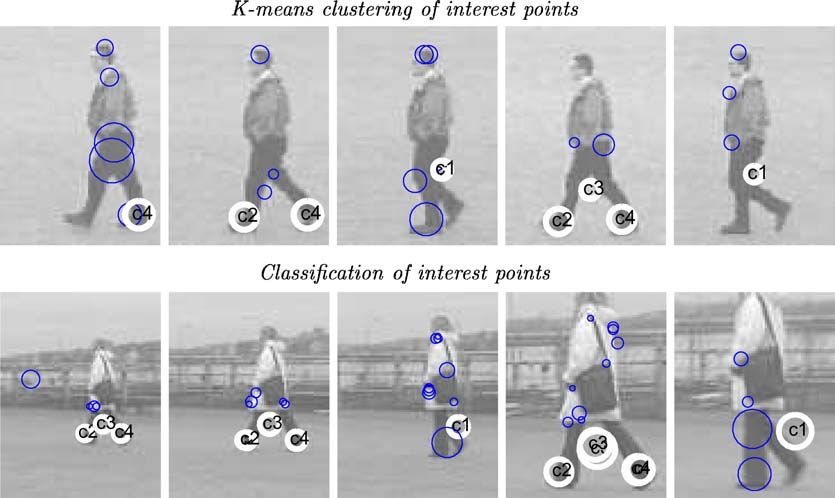
108       Laptev

Figure 1. Result of detecting the strongest spatio-temporal interest points in a football sequence with a player heading the ball (a) and in a
hand clapping sequence (b). From the temporal slices of space-time volumes shown here, it is evident that the detected events correspond to
neighborhoods with high spatio-temporal variation in the image data or “space-time corners”.

   In the spatial domain, points with a significant lo-                   As events often have characteristic extents in both
cal variation of image intensities have been exten-                       space and time (Koenderink, 1988; Lindeberg and
sively investigated in the past (Förstner and Gülch,                    Fagerström, 1996; Florack, 1997; Lindeberg, 1997;
1987; Harris and Stephens, 1988; Lindeberg, 1998;                         Chomat et al., 2000b; Zelnik-Manor and Irani, 2001),
Schmid et al., 2000). Such image points are frequently                    we investigate the behavior of interest points in spatio-
referred to as “interest points” and are attractive due                   temporal scale-space and adapt both the spatial and the
to their high information contents and relative sta-                      temporal scales of the detected features in Section 3.
bility with respect to perspective transformations of                     In Section 4, we show how the neighborhoods of inter-
the data. Highly successful applications of interest                      est points can be described in terms of spatio-temporal
points have been presented for image indexing (Schmid                     derivatives and then be used to distinguish different
and Mohr, 1997), stereo matching (Tuytelaars and                          events in video. In Section 5, we consider a video repre-
Van Gool, 2000; Mikolajczyk and Schmid, 2002; Tell                        sentation in terms of classified spatio-temporal interest
and Carlsson, 2002), optic flow estimation and track-                     points and demonstrate how this representation can be
ing (Smith and Brady, 1995; Bretzner and Lindeberg,                       efficient for the task of video registration. In particular,
1998), and object recognition (Lowe, 1999; Hall et al.,                   we present an approach for detecting walking people
2000; Fergus et al., 2003; Wallraven et al., 2003).                       in complex scenes with occlusions and dynamic back-
   In this paper, we extend the notion of interest points                 ground. Finally, Section 6 concludes the paper with the
into the spatio-temporal domain and show that the re-                     summary and discussion.
sulting local space-time features often correspond to
interesting events in video data (see Fig. 1). In par-
ticular, we aim at a direct scheme for event detection
and interpretation that does not require feature track-                   2.     Spatio-Temporal Interest Point Detection
ing, segmentation nor computation of optic flow. In the
considered sample application we show that the pro-                       2.1.    Interest Points in the Spatial Domain
posed type of features can be used for sparse coding of
video information that in turn can be used for interpret-                 In the spatial domain, we can model an image f sp :
ing video scenes such as human motion in situations                       R2 → R by its linear scale-space representation
with complex and non-stationary background.                               (Witkin, 1983; Koenderink and van Doorn, 1992;
   To detect spatio-temporal interest points, we build on                 Lindeberg, 1994; Florack, 1997) L sp : R2 × R+ → R
the idea of the Harris and Förstner interest point oper-
ators (Harris and Stephens, 1988; Förstner and Gülch,

1987) and describe the detection method in Section 2.                            L sp x, y; σl2 = g sp x, y; σl2 ∗ f sp (x, y),           (1)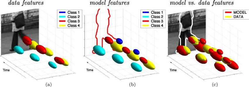
On Space-Time Interest Points        109

defined by the convolution of f sp with Gaussian ker-           The result of detecting Harris interest points in an
nels of variance σl2                                          outdoor image sequence of a walking person is pre-
                                                              sented at the bottom row of Fig. 8.
                   1
g sp x, y; σl2 =       2
                         exp − (x 2 + y 2 ) 2σl2 . (2)
                   2πσl

The idea of the Harris interest point detector is to find     2.2.   Interest Points in the Spatio-Temporal Domain
spatial locations where f sp has significant changes in
both directions. For a given scale of observation σl2 ,       In this section, we develop an operator that responds
such points can be found using a second moment matrix         to events in temporal image sequences at specific lo-
integrated over a Gaussian window with variance σi2           cations and with specific extents in space-time. The
(Förstner and Gülch, 1987; Bigün et al., 1991; Gårding    idea is to extend the notion of interest points in the
and Lindeberg, 1996):                                         spatial domain by requiring the image values in local
                                                              spatio-temporal volumes to have large variations along
                                                          both the spatial and the temporal directions. Points with
 µsp ·; σl2 , σi2 = g sp ·; σi2
                                      T             such properties will correspond to spatial interest points
                     ∗ ∇ L ·; σl2 ∇ L ·; σl2                  with distinct locations in time corresponding to lo-
                                   sp 2    sp sp          cal spatio-temporal neighborhoods with non-constant
                                   Lx    Lx Ly
                   = g ·; σi ∗
                      sp      2
                                     sp sp  sp 2            motion.
                                    Lx Ly    Ly                  To model a spatio-temporal image sequence, we use
                                                    (3)       a function f : R2 × R → R and construct its linear
                                                              scale-space representation L: R2 × R × R2+ → R by
                                                        sp
where ‘∗’ denotes the convolution operator, and L x           convolution of f with an anisotropic Gaussian kernel1
       sp
and L y are Gaussian derivatives computed at local            with independent spatial variance σl2 and temporal vari-
                           sp
scale σl2 according to L x = ∂x (g sp (·; σl2 ) ∗ f sp (·))   ance τl2
       sp
and L y = ∂ y (g (·; σl ) ∗ f sp (·)). The second mo-
                  sp     2

ment descriptor can be thought of as the covariance
matrix of a two-dimensional distribution of image ori-                  L ·; σl2 , τl2 = g ·; σl2 , τl2 ∗ f (·),    (5)
entations in the local neighborhood of a point. Hence,
the eigenvalues λ1 , λ2 , (λ1 ≤ λ2 ) of µsp constitute
descriptors of variations in f sp along the two image         where the spatio-temporal separable Gaussian kernel
directions. Specifically, two significantly large values      is defined as
of λ1 , λ2 indicate the presence of an interest point.
To detect such points, Harris and Stephens (1988)                                                  1
proposed to detect positive maxima of the corner                      g x, y, t; σl2 , τl2 =
function                                                                                    (2π )3 σl4 τl2

                                                                        × exp − (x 2 + y 2 ) 2σl2 − t 2 2τl2 .      (6)
            H sp = det(µsp ) − k trace2 (µsp )
                 = λ1 λ2 − k(λ1 + λ2 )2 .              (4)
                                                              Using a separate scale parameter for the temporal do-
At the positions of the interest points, the ratio of the     main is essential, since the spatial and the temporal ex-
eigenvalues α = λ2 /λ1 has to be high. From (4) it fol-       tents of events are in general independent. Moreover,
lows that for positive local maxima of H sp , the ratio α     as will be illustrated in Section 2.3, events detected us-
has to satisfy k ≤ α/(1+α)2 . Hence, if we set k = 0.25,      ing our interest point operator depend on both the spa-
the positive maxima of H will only correspond to ide-         tial and the temporal scales of observation and, hence,
ally isotropic interest points with α = 1, i.e. λ1 = λ2 .     require separate treatment of the corresponding scale
Lower values of k allow us to detect interest points with     parameters σl2 and τl2 .
more elongated shape, corresponding to higher values             Similar to the spatial domain, we consider a spatio-
of α. A commonly used value of k in the literature is         temporal second-moment matrix, which is a 3-by-3 ma-
k = 0.04 corresponding to the detection of points with        trix composed of first order spatial and temporal deriva-
α < 23.                                                       tives averaged using a Gaussian weighting function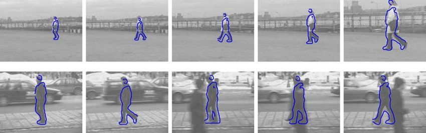
110 Laptev
g(·; σi2 , τi2 ) For clarity of presentation, we show the spatio-
temporal data as 3-D space-time plots, where the orig-
L 2x Lx Ly Lx Lt inal signal is represented by a threshold surface, while
the detected interest points are illustrated by ellipsoids
µ = g ·; σi2 , τi2 ∗ L x L y L 2y L y Lt , (7)
with positions corresponding to the space-time location
Lx Lt L y Lt L 2t
of the interest point and the length of the semi-axes pro-
portional to the local scale parameters σl and τl used in
where we here relate the integration scales σi2 and τi2 to
the computation of H .
the local scales σl2 and τl2 according to σi2 = sσl2 and
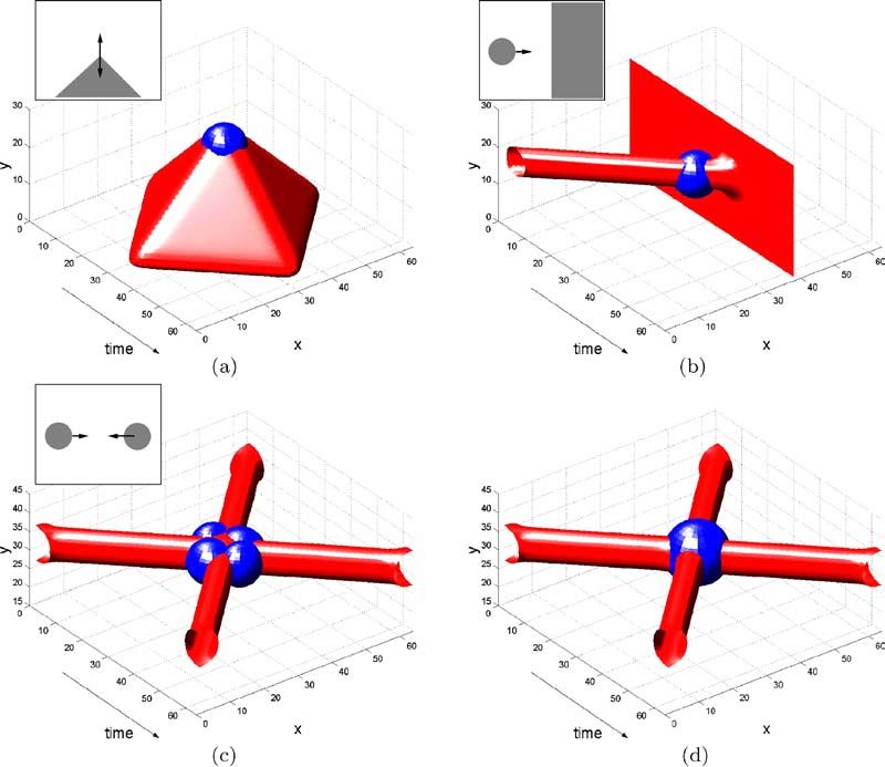
Figure 2(a) shows a sequence with a moving corner.
τi2 = sτl2 . The first-order derivatives are defined as
The interest point is detected at the moment in time
when the motion of the corner changes direction. This
L x ·; σl2 , τl2 = ∂x (g ∗ f ),
type of event occurs frequently in natural sequences,
L y ·; σl2 , τl2 = ∂ y (g ∗ f ), such as sequences of articulated motion. Note that ac-
cording to the definition of spatio-temporal interest
L t ·; σl2 , τl2 = ∂t (g ∗ f ).
points, image structures with constant motion do not
To detect interest points, we search for regions in f give rise to responses of the detector. Other typical
having significant eigenvalues λ1 , λ2 , λ3 of µ. Among types of events that can be detected by the proposed
different approaches to find such regions, we propose method are splits and unifications of image structures.
here to extend the Harris corner function (4) defined In Fig. 2(b), the interest point is detected at the mo-
for the spatial domain into the spatio-temporal domain ment and the position corresponding to the collision of
by combining the determinant and the trace of µ as a ball and a wall. Similarly, interest points are detected
follows: at the moment of collision and bouncing of two balls
as shown in Fig. 2(c)–(d). Note, that different types of
H = det(µ) − k trace3 (µ) events are detected depending on the scale of observa-
tion.
= λ1 λ2 λ3 − k(λ1 + λ2 + λ3 )3 . (8) To further emphasize the importance of the spatial
and the temporal scales of observation, let us consider
To show how positive local maxima of H correspond to an oscillating signal with different spatial and tem-
points with high values of λ1 , λ2 , λ3 (λ1 ≤ λ2 ≤ λ3 ), poral frequencies defined by f (x, y, t) = sgn(y −
we define the ratios α = λ2 /λ1 and β = λ3 /λ1 and sin(x 4 ) sin(t 4 )), where sgn(u) = 1 for u > 0 and
re-write H as sgn(u) = −1 for u < 0 (see Fig. 3). As can be
seen from the illustration, the result of detecting the
H = λ31 (αβ − k(1 + α + β)3 ). strongest interest points highly depends on the choice
of the scale parameters σl2 and τl2 . We can observe that
From the requirement H ≥ 0, we get k ≤ αβ/(1 + α + space-time structures with long temporal extents are
β)3 and it follows that k assumes its maximum possi- detected for large values of τl2 while short events are
ble value k = 1/27 when α = β = 1. For sufficiently preferred by the detector with small values of τl2 . Sim-
large values of k, positive local maxima of H corre- ilarly, the spatial extent of the events is related to the
spond to points with high variation of the image values value of the spatial scale parameter σl2 .
along both the spatial and the temporal directions. In From the presented examples, we can conclude
particular, if we set the maximum value of α, β to 23 as that a correct selection of temporal and spatial scales
in the spatial domain, the value of k to be used in H (8) is crucial when capturing events with different spa-
will then be k ≈ 0.005. Thus, spatio-temporal interest tial and temporal extents. Moreover, estimating the
points of f can be found by detecting local positive spatio-temporal extents of events is important for
spatio-temporal maxima in H . their further interpretation. In the next section, we
will present a mechanism for simultaneous esti-
2.3. Experimental Results for Synthetic Data mation of spatio-temporal scales. This mechanism
will then be combined with the interest point de-
In this section, we illustrate the detection of spatio- tector resulting in scale-adapted interest points in
temporal interest points on synthetic image sequences. Section 3.2.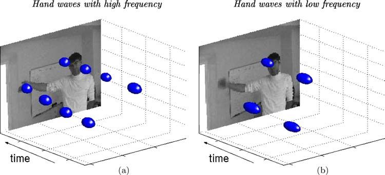
On Space-Time Interest Points                 111

Figure 2. Results of detecting spatio-temporal interest points on synthetic image sequences. (a) A moving corner; (b) A merge of a ball and
a wall; (c) Collision of two balls with interest points detected at scales σl2 = 8 and τl2 = 8; (d) the same signal as in (c) but with the interest
points detected at coarser scales σl2 = 16 and τl2 = 16.

3.     Spatio-Temporal Scale Adaptation                                         For the purpose of analysis, we will first study a pro-
                                                                             totype event represented by a spatio-temporal Gaussian
3.1.    Scale Selection in Space-Time                                        blob

During recent years, the problem of automatic scale                                                                      1
                                                                                         f x, y, t; σ02 , τ02 =
selection has been addressed in several different ways,
                                                                                                                (2π )3 σl4 τl2
based on the maximization of normalized derivative
expressions over scale, or the behavior of entropy mea-                                    × exp −(x 2 + y 2 ) 2σ02 − t 2 2τ02
sures or error measures over scales (see Lindeberg and
Bretzner (2003) for a review). To estimate the spatio-                       with spatial variance σ02 and temporal variance τ02
temporal extent of an event in space-time, we follow                         (see Fig. 4(a)). Using the semi-group property of the
works on local scale selection proposed in the spatial                       Gaussian kernel, it follows that the scale-space repre-
domain by Lindeberg (1998) as well as in the temporal                        sentation of f is
domain (Lindeberg, 1997). The idea is to define a dif-
ferential operator that assumes simultaneous extrema
over spatial and temporal scales that are characteristic                             L(·; σ 2 , τ 2 ) = g(·; σ 2 , τ 2 ) ∗ f ·; σ02 , τ02

for an event with a particular spatio-temporal location.                                              = g ·; σ02 + σ 2 , τ02 + τ 2 .
112 Laptev
Figure 3. Results of detecting interest point at different spatial and temporal scales for a synthetic sequence with impulses having varying
extents in space and time. The extents of the detected events roughly corresponds to the scale parameters σl2 and τl2 used for computing H (8).
To recover the spatio-temporal extent (σ0 , τ0 ) of f , we The idea of scale selection we follow here is to de-
consider second-order derivatives of L normalized by termine the parameters a, b, c, d such that L x x,nor m ,
the scale parameters as follows L yy,nor m and L tt,nor m assume extrema at scales σ̃ 2 = σ02
and τ̃ 2 = τ02 . To find such extrema, we differentiate the
expressions in (9) with respect to the spatial and the
L x x,nor m = σ 2a τ 2b L x x ,
temporal scale parameters. For the spatial derivatives
L yy,nor m = σ 2a τ 2b L yy , we obtain the following expressions at the center of the
L tt,nor m = σ 2c τ 2d L tt . (9) blob
∂
[L x x,nor m (0, 0, 0; σ 2 , τ 2 )]
All of these entities assume local extrema over space ∂σ 2
and time at the center of the blob f . Moreover, depend- aσ 2 − 2σ 2 + aσ02
ing on the parameters a, b and c, d, they also assume = − 2 6 2 σ τ
2(a−1) 2b
local extrema over scales at certain spatial and temporal (2π ) σ0 + σ
3 2 τ0 + τ 2
scales, σ̃ 2 and τ̃ 2 . (10)On Space-Time Interest Points 113
Figure 4. (a) A Spatio-temporal Gaussian blob with spatial variance σ02 = 4 and temporal variance τ02 = 16; (b)–(c) derivatives of ∇nor 2
mL
2 2
with respect to scales. The zero-crossings of (∇nor m L)σ 2 and (∇nor m L)τ 2 indicate extrema of ∇nor m L at scales corresponding to the spatial and
2
the temporal extents of the blob.
∂ ∂
[L x x,nor m (0, 0, 0; σ 2 , τ 2 )] [L tt,nor m (0, 0, 0; σ 2 , τ 2 )]
∂τ 2 ∂τ 2
2bτ02 + 2bτ 2 − τ 2 2dτ02 + 2dτ 2 − 3τ 2
= − 2 4 2 3 τ σ .
2(b−1) 2a
= − 2 2 2 5 τ σ
2(d−1) 2c
2 π σ0 + σ
5 3 2 τ0 + τ 2 2 π σ0 + σ
5 3 2 τ0 + τ 2
(11) (13)
By setting these expressions to zero, we obtain the fol- leads to the expressions
lowing simple relations for a and b
cσ 2 − 2σ 2 + cσ02 = 0, 2dτ02 + 2dτ 2 − τ 2 = 0
aσ 2 − 2σ 2 + aσ02 = 0, 2bτ02 + 2bτ 2 − τ 2 = 0 which after substituting σ 2 = σ02 and τ 2 = τ02 result in
c = 1/2 and d = 3/4.
which after substituting σ 2 = σ02 and τ 2 = τ02 lead The normalization of derivatives in (9) guarantees
to a = 1 and b = 1/4. Similarly, differentiating the that all these partial derivative expressions assume local
second-order temporal derivative space-time-scale extrema at the center of the blob f and
at scales corresponding to the spatial and the temporal
∂ extents of f , i.e. σ = σ0 and τ = τ0 . From the sum of
[L tt,nor m (0, 0, 0; σ 2 , τ 2 )] these partial derivatives, we then define a normalized
∂σ 2
spatio-temporal Laplace operator according to
cσ 2 − σ 2 + cσ02
= − σ 2(c−1) τ 2d
(2π ) (σ0 + σ ) (τ0 + τ )
3 2 2 4 2 2 3 ∇nor
2
m L = L x x,nor m + L yy,nor m + L tt,nor m
(12) = σ 2 τ 1/2 (L x x + L yy ) + σ τ 3/2 L tt . (14)114 Laptev
Figures 4(b) and (c) show derivatives of this opera- Here, we extend this idea and detect interest points
tor with respect to the scale parameters evaluated at the that are simultaneous maxima of the spatio-temporal
center of a spatio-temporal blob with spatial variance corner function H (8) over space and time (x, y, t)
σ02 = 4 and temporal variance τ02 = 16. The zero- as well as extrema of the normalized spatio-temporal
crossings of the curves verify that ∇nor
2
m L assumes ex- Laplace operator ∇nor2
m L (14) over scales (σ , τ ). One
2 2
trema at the scales σ = σ0 and τ = τ02 . Hence, the
2 2 2
way of detecting such points is to compute space-time
spatio-temporal extent of the Gaussian prototype can be maxima of H for each spatio-temporal scale level and
estimated by finding the extrema of ∇nor 2
m L over both then to select points that maximize (∇nor 2 2
m L) at the
spatial and temporal scales. In the following section, corresponding scale. This approach, however, requires
we will use this operator for estimating the extents of dense sampling over the scale parameters and is there-
other spatio-temporal structures, in analogy with pre- fore computationally expensive.
vious work of using the normalized Laplacian operator An alternative we follow here, is to detect interest
as a general tool for estimating the spatial extent of points for a set of sparsely distributed scale values and
image structures in the spatial domain. then to track these points in the spatio-temporal scale-
time-space towards the extrema of ∇nor 2
m L. We do this
by iteratively updating the scale and the position of the
3.2. Scale-Adapted Space-Time Interest Points interest points by (i) selecting the neighboring spatio-
2 2
temporal scale that maximizes (∇nor m L) and (ii) re-
Local scale estimation using the normalized Laplace detecting the space-time location of the interest point at
operator has shown to be very useful in the spatial a new scale. Thus, instead of performing a simultaneous
domain (Lindeberg, 1998; Almansa and Lindeberg, maximization of H and ∇nor 2
m L over five dimensions
2000; Chomat et al., 2000a). In particular, Mikolajczyk (x, y, t, σ , τ ), we implement the detection of local
2 2
and Schmid (2001) combined the Harris interest point maxima by splitting the space-time dimensions (x, y, t)
operator with the normalized Laplace operator and de- and scale dimensions (σ 2 , τ 2 ) and iteratively optimiz-
rived a scale-invariant Harris-Laplace interest point de- ing over the subspaces until the convergence has been
tector. The idea is to find points in scale-space that are reached.2 The corresponding algorithm is presented in
both spatial maxima of the Harris function H sp (4) and Fig. 5.
extrema over scale of the scale-normalized Laplace op- The result of scale-adaptation of interest points for
erator in space. the spatio-temporal pattern in Fig. 3 is shown in Fig. 6.
Figure 5. Algorithm for scale adaption of spatio-temporal interest points.On Space-Time Interest Points 115
video sequences. In real-time situations, when us-
ing causal scale-space representation based on re-
cursive temporal filters (Lindeberg and Fagerström,
1996; Lindeberg, 2002), only a fixed set of discrete
temporal scales is available at any moment. In that
case an approximate estimate of temporal scale can
still be found by choosing interest points that maxi-
2 2
mize (∇nor m L) in a local neighborhood of the spatio-
temporal scale-space; see also (Lindeberg, 1997) for a
treatment of automatic scale selection for time-causal
scale-spaces.
3.3. Experiments
In this section, we investigate the performance of the
Figure 6. The result of scale-adaptation of spatio-temporal interest proposed scale-adapted spatio-temporal interest point
points computed from a space-time pattern of the form f (x, y, t) = detector applied to real image sequences. In the first
sgn(y − sin(x 4 ) ∗ sin(t 4 )). The interest points are illustrated as el-
lipsoids showing the selected spatio-temporal scales overlayed on a
example, we consider a sequence of a walking person
surface plot of the intensity landscape. with non-constant image velocities due to the oscil-
lating motion of the legs. As can be seen in Fig. 7,
As can be seen, the chosen scales of the adapted in- the spatio-temporal image pattern gives rise to stable
terest points match the spatio-temporal extents of the interest points. Note that the detected interest points
corresponding structures in the pattern. reflect well-localized events in both space and time,
It should be noted, however, that the presented algo- corresponding to specific space-time structures of the
rithm has been developed for processing pre-recorded leg. From the space-time plot in Fig. 7(a), we can
Figure 7. Results of detecting spatio-temporal interest points from the motion of the legs of a walking person. (a) 3-D plot with a thresholded
level surface of a leg pattern (here shown upside down to simplify interpretation) and the detected interest points illustrated by ellipsoids; (b)
spatio-temporal interest points overlayed on single frames in the original sequence.116 Laptev Figure 8. Top: Results of spatio-temporal interest point detection for a zoom-in sequence of a walking person. The spatial scale of the detected points (corresponding to the size of circles) matches the increasing spatial extent of the image structures and verifies the invariance of the interest points with respect to changes in spatial scale. Bottom: Pure spatial interest point detector (here, Harris-Laplace, Mikolajczyk and Schmid, 2001) selects both moving and stationary points in the image sequence. also observe how the selected spatial and temporal points are detected at the moments and at the spatial po- scales of the detected features roughly match the spatio- sitions where the palm of a hand changes its direction temporal extents of the corresponding image structures. of motion. Whereas the spatial scale of the detected The top rows of Fig. 8 show interest points detected interest points remains constant, the selected temporal in an outdoor sequence with a walking person and a scale depends on the frequency of the wave pattern. zooming camera. The changing values of the selected The high frequency pattern results in short events and spatial scales (illustrated by the size of the circles) il- gives rise to interest points with small temporal extent lustrate the invariance of the method with respect to (see Fig. 9(a)). Correspondingly, hand motions with spatial scale changes of the image structures. Note that low frequency result in interest points with long tem- besides events in the leg pattern, the detector finds spu- poral extent as shown in Fig. 9(b). rious points due to the non-constant motion of the coat and the arms. Image structures with constant motion in 4. Classification of Events the background, however, do not result in the response of the detector. The pure spatial interest operator3 on The detected interest points have significant variations the contrary gives strong responses in the static back- of image values in a local spatio-temporal neighbor- ground as shown at the bottom row of Fig. 8. hood. To differentiate events from each other and from The third example explicitly illustrates how the pro- noise, one approach is to compare local neighbor- posed method is able to estimate the temporal extent hoods and assign points with similar neighborhoods of detected events. Figure 9 shows a person making to the same class of events. A similar approach has hand-waving gestures with a high frequency on the left proven to be highly successful in the spatial domain for and a low frequency on the right. The distinct interest the task of image representation (Malik et al., 1999)
On Space-Time Interest Points          117

Figure 9. Result of interest point detection for a sequence with waving hand gestures: (a) Interest points for hand movements with high
frequency; (b) Interest points for hand movements with low frequency.

indexing (Schmid and Mohr, 1997) and recogni-                                      point descriptors and detect groups of points with sim-
tion (Hall et al., 2000; Weber et al., 2000; Leung and                             ilar spatio-temporal neighborhoods. Thus clustering of
Malik, 2001). In the spatio-temporal domain, local de-                             spatio-temporal neighborhoods is similar to the idea
scriptors have been previously used by Chomat et al.                               of textons (Malik et al., 1999) used to describe image
(2000b) and others.                                                                texture as well as to detect object parts for spatial recog-
   To describe a spatio-temporal neighborhood, we                                  nition (Weber et al., 2000). Given training sequences
consider normalized spatio-temporal Gaussian deriva-                               with periodic motion, we can expect repeating events
tives defined as                                                                   to give rise to populated clusters. On the contrary, spo-
                                                                                   radic interest points can be expected to be sparsely dis-
             L x m y n t k = σ m+n τ k (∂x m y n t k g) ∗ f,                (15)   tributed over the descriptor space giving rise to weakly
                                                                                   populated clusters. To test this idea we applied k-means
computed at the scales used for detecting the corre-                               clustering with k = 15 to the sequence of a walking
sponding interest points. The normalization with re-                               person in the upper row of Fig. 11. We found out that
spect to scale parameters guarantees the invariance of                             the four most densely populated clusters c1, . . . , c4 in-
the derivative responses with respect to image scalings                            deed corresponded to stable interest points of the gait
in both the spatial domain and the temporal domain.                                pattern. Local spatio-temporal neighborhoods of these
Using derivatives, we define event descriptors from                                points are shown in Fig. 10, where we can confirm the
the third order local jet4 (Koenderink and van Doorn,                              similarity of patterns inside the clusters and their dif-
1987) computed at spatio-temporal scales determined                                ference between clusters.
from the detection scales of the corresponding interest                               To represent characteristic repetitiveevents   in video,
points                                                                             we compute cluster means m i = n1i nk=1      i
                                                                                                                                   jk for each
                                                                                   significant cluster ci consisting of n i points. Then,
    j = (L x , L y , L t , L x x , . . . , L ttt )                          (16)   in order to classify an event on an unseen sequence,
                                                     σ 2 =σ̃i2 ,τ 2 =τ̃i2
                                                                                   we assign the detected point to the cluster ci that
To compare two events, we compute the Mahalanobis                                  minimizes the distance d(m i , j0 ) (17) between the jet
distance between their descriptors as                                              of the interest point j0 and the cluster mean m i . If
                                                                                   the distance is above a threshold, the point is clas-
         d 2 ( j1 , j2 ) = ( j1 − j2 ) −1 ( j1 − j2 )T ,                   (17)   sified as background. An application of this classifi-
                                                                                   cation scheme is demonstrated in the second row of
where  is a covariance matrix corresponding to the                                Fig. 11. As can be seen, most of the points corre-
typical distribution of interest points in training data.                          sponding to the gait pattern are correctly classified,
  To detect similar events in the data, we apply                                   while the other interest points are discarded. Observe
k-means clustering (Duda et al., 2001) in the space of                             that the person in the second sequence of Fig. 11
118 Laptev Figure 10. Local spatio-temporal neighborhoods of interest points corresponding to the first four most populated clusters obtained from a sequence of walking person. Figure 11. Interest points detected for sequences of walking persons. First row: the result of clustering spatio-temporal interest points in training data. The labelled points correspond to the four most populated clusters; Second row: the result of classifying interest points with respect to the clusters found in the first sequence.
On Space-Time Interest Points                119

Figure 12. Matching of spatio-temporal data features with model features: (a) Features detected from the data sequence over a time interval
corresponding to three periods of the gait cycle; (b) Model features minimizing the distance to the features in (a); (c) Model features and data
features overlaid. The estimated silhouette overlayed on the current frame confirms the correctness of the method.

undergoes significant size changes in the image. Due                       tures of the data inside a spatio-temporal window (see
to the scale-invariance of the interest points as well as                  Fig. 12).
their jet responses, the size transformations do not ef-
fect neither the result of event detection nor the result of
classification.                                                            5.1.    Walking Model

                                                                           To obtain a model of a walking person, we consider
5.   Application to Video Interpretation                                   the upper sequence in Fig. 11 and manually select a
                                                                           time interval (t0 , t0 + T ) corresponding to the period
In this section, we illustrate how a sparse representa-                    T of the gait pattern. Then, given n features f im =
tion of video sequences by classified spatio-temporal                      (xim , yim , tim , σim , τim , cim ), i = 1, . . . , n (m stands for
interest points can be used for video interpretation. We                   model) defined by the positions (xim , yim , tim ), scales
consider the problem of detecting walking people and                       (σim , τim ) and classes cim of interest points detected in
estimating their poses when viewed from the side in                        the selected time interval, i.e. tim ∈ (t0 , t0 + T ), we
outdoor scenes. Such a task is complicated, since the                      define the walking model by a set of periodically re-
variations in appearance of people together with the                       peating features M = { f i + (0, 0, kT, 0, 0, 0, 0) | i =
variations in the background may lead to ambiguous                         1, . . . , n, k ∈ Z}. Furthermore, to account for varia-
interpretations. Human motion is a strong cue that has                     tions of the position and the size of a person in the
been used to resolve this ambiguity in a number of pre-                    image, we introduce a state for the model determined
vious works. Some of the works rely on pure spatial                        by the vector X = (x, y, θ, s, ξ, vx , v y , vs ). The com-
image features while using sophisticated body mod-                         ponents of X describe the position of the person in the
els and tracking schemes to constrain the interpreta-                      image (x, y), his size s, the frequency of the gait ξ ,
tion (Baumberg and Hogg, 1996; Bregler and Malik,                          the phase of the gait cycle θ at the current time mo-
1998; Sidenbladh et al., 2000). Other approaches use                       ment as well as the temporal variations (vx , v y , vs ) of
spatio-temporal image cues such as optical flow (Black                     (x, y, s); vx and v y describe the velocity in the image
et al., 1997) or motion templates (Baumberg and Hogg,                      domain, while vs describes how fast size changes oc-
1996; Efros et al., 2003). The work of Niyogi and                          cur. Given the state X , the parameters of each model
Adelson (1994) concerns the structure of the spatio-                       feature f ∈ M transform according to
temporal gait pattern and is closer to ours.
   The idea of the following approach is to represent                          x̃ m = x + sx m + ξ vx (t m + θ ) + sξ x m vs (t m + θ )
both the model and the data using local and discrimi-
native spatio-temporal features and to match the model                         ỹ m = y + sy m + ξ v y (t m + θ ) + sξ y m vs (t m + θ )
by matching its features to the correspondent fea-                             t̃ m = ξ (t m + θ )
120 Laptev
σ̃ m = sσ m + vs sσ m (t m + θ) (18) Here, the distance between features of different classes
τ̃ m
= ξτ m is regarded as infinite. Alternatively, one could mea-
sure the feature distance by taking into account their
c̃ = cm
m
descriptors and distances from several of the nearest
cluster means.
It follows that this type of scheme is able to handle To find the best match between the model and the
translations and uniform rescalings in the image do- data, we search for the model state X̃ that minimizes
main as well as uniform rescalings in the temporal do- H in (19)
main. Hence, it allows for matching of patterns with
different image velocities as well as with different fre-
quencies over time. X̃ = argmin H( M̃(X ), D, t0 ) (21)
X
To estimate the boundary of the person, we extract
silhouettes S = {x s , y s , θ s | θ s = 1, . . . , T } on the
model sequence (see Fig. 11) one for each frame cor- using a standard Gauss-Newton optimization method.
responding to the discrete value of the phase parameter The result of such an optimization for a sequence with
θ . The silhouette is used here only for visualization pur- data features in Fig. 12(a) is illustrated in Fig. 12(b).
pose and allows us to approximate the boundary of the Here, the match between the model and the data fea-
person in the current frame using the model state X and tures was searched over a time window corresponding
a set of points {(x s , y s , θ s ) ∈ S | θ s = θ } transformed to three periods of the gait pattern or approximately
according to x̃ s = sx s + x, ỹ s = sy s + y. 2 seconds of video. As can be seen from Fig. 12(c),
the overlaps between the model features and the data
features confirm the match between the model and the
5.2. Model Matching data. Moreover, the model silhouette transformed ac-
cording to X̃ matches with the contours of the person
Given a model state X , a current time t0 , a length in the current frame and confirms a reasonable estimate
of the time window tw , and a set of data features of the model parameters.
D = { f d = (x d , y d , t d , σ d , τ d , cd ) | t d ∈ (t0 , t0 − tw )}
detected from the recent time window of the data se-
quence, the match between the model and the data is 5.3. Results
defined by a weighted sum of distances h between the
model features f im and the data features f jd Figure 13 presents results of the described approach
applied to two outdoor sequences. The first sequence
n
h f̃ im , f jd e−(t̃i −t0 ) /ξ , illustrates the invariance of the method with respect
m 2
H( M̃(X ), D, t0 ) = (19)
i to size variations of the person in the image plane.
The second sequence shows the successful detection
where M̃(X ) is a set of n model features in the time and pose estimation of a person despite the presence
window (t0 , t0 − tw ) transformed according to (18), of a complex non-stationary background and occlu-
i.e. M̃ = { f̃ m |t m ∈ (t0 , t0 − tw )}, f jd ∈ D is a data sions. Note that these results have been obtained by
feature minimizing the distance h for a given f im and re-initializing model parameters before optimization
ξ is the variance of the exponential weighting function at each frame. Hence, the approach is highly stable
that gives more importance to recent features. and could be improved further by tracking the model
The distance h between two features of the same parameters X̃ over time.
class is defined as a Euclidean distance between two The need for careful initialization and/or simple
points in space-time, where the spatial and the temporal background are frequent obstacles in previous ap-
dimensions are weighted with respect to a parameter ν proaches for human motion analysis. The success of
as well as by the extents of the features in space-time our method is due to the low ambiguity and simplicity
of the matching scheme originating from the distinct
(x m − x d )2 + (y m − y d )2 and stable nature of the spatio-temporal features. In this
h 2 ( f m , f d ) = (1 − ν)
(σ m )2 respect, we want to propose direct detection of spatio-
(t − t )
m d 2 temporal events as an interesting alternative when rep-
+ν . (20) resenting and interpreting video data.
(τ m )2On Space-Time Interest Points 121
Figure 13. The result of matching a spatio-temporal walking model to sequences of outdoor scenes.
6. Summary direction of motion, changes in image contrast and ro-
tations.
We have described an interest point detector that finds
local image features in space-time characterized by a Acknowledgments
high variation of the image values in space and non-
constant motion over time. From the presented exam- This paper is based on two presentations held at Scale-
ples, it follows that many of the detected points in- Space’03 in Isle of Skye and at ICCV’03 in Nice Laptev
deed correspond to meaningful events. Moreover, we and Lindeberg (2003a, 2003b).
propose local maximization of the normalized spatio- The support from the Swedish Research Council
temporal Laplacian operator as a general tool for scale is gratefully acknowledged. The author would like to
selection in space-time. Using this mechanism, we es- thank Tony Lindeberg for many valuable discussions
timated characteristic spatio-temporal extents of de- concerning this work. The author is also grateful to
tected events and computed their scale-invariant spatio- Anastasiya Syromyatnikova and Carsten Rother for
temporal descriptors. their help in experiments.
Using scale-adapted descriptors in terms of N -jets
we then addressed the problem of event classifica-
tion and illustrated how classified spatio-temporal in- Notes
terest points constitute distinct and stable descriptors
1. For real-time applications, convolution with a Gaussian kernel
of events in video, which can be used for video rep- in the temporal domain violates causality constraints, since the
resentation and interpretation. In particular, we have temporal image data is available only for the past. To solve this
shown how a video representation by spatio-temporal problem, time-causal scale-space filters can be used to satisfy the
interest points enables detection and pose estimation causality constraints (Koenderink, 1988; Lindeberg and Fager-
of walking people in the presence of occlusions and ström, 1996; Florack, 1997; Lindeberg, 2002). In this paper, we
assume that the data is available for a sufficiently long period
highly cluttered and dynamic background. Note that of time and that the image sequence can be convolved with a
this result was obtained using a standard optimiza- Gaussian kernel over both space and time.
tion method without careful manual initialization or 2. For the experiments presented in this paper, with image sequences
tracking. of spatial resolution 160 × 120 pixels and temporal sampling
In future work, we plan to extend application of in- frequency 25 Hz (totally up to 200 frames per sequence), we
initialized the detection of interest points using combinations of
terest points to the field of motion-based recognition. spatial scales σl2 = [2, 4, 8] and temporal scales σl2 = [2, 4, 8],
Moreover, as the current scheme of event detection while using s = 2 for the ratio between the integration and the
is not invariant under Galilean transformations, future local scale when computing the second-moment matrix.
work should investigate the possibilities of including 3. Here, we used the scale-adapted Harris interest point detector
such invariance and making the approach independent (Mikolajczyk and Schmid, 2001) that detects maxima of H sp (4)
in space and extrema of normalized Laplacian operator over
of the relative camera motion (Laptev and Lindeberg, scales (Lindeberg, 1998).
2002). Another extension should consider the invari- 4. Note that our representation is currently not invariant with re-
ance of spatio-temporal descriptors with respect to the spect to planar image rotations. Such invariance could be added122 Laptev
by considering steerable derivatives or rotationally invariant op- Int. Soc. for Photogrammetry and Remote Sensing, Interlaken,
erators in space. Switzerland.
Gårding, J. and Lindeberg, T. 1996. Direct computation of shape
References cues using scale-adapted spatial derivative operators. International
Journal of Computer Vision, 17(2):163–191.
Almansa, A. and Lindeberg, T. 2000. Fingerprint enhancement by Hall, D., de Verdiere, V., and Crowley, J. 2000. Object recognition
shape adaptation of scale-space operators with automatic scale- using coloured receptive fields. In Proc. Sixth European Confer-
selection. IEEE Transactions on Image Processing, 9(12):2027– ence on Computer Vision, Vol. 1842 of Lecture Notes in Com-
2042. puter Science, Springer Verlag, Berlin, Dublin, Ireland, pp. I:164–
Barron, J., Fleet, D., and Beauchemin, S. 1994. Performance of op- 177.
tical flow techniques. International Journal of Computer Vision, Harris, C. and Stephens, M. 1988. A combined corner and edge
12(1):43–77. detector. Alvey Vision Conference, pp. 147–152.
Baumberg, A.M. and Hogg, D. 1996. Generating spatiotemporal Hoey, J. and Little, J. 2000. Representation and recognition of com-
models from examples. Image and Vision Computing, 14(8):525– plex human motion. In Proc. Computer Vision and Pattern Recog-
532. nition, Hilton Head, SC, pp. I:752–759.
Bigün, J., Granlund, G., and Wiklund, J. 1991. Multidimensional Koenderink, J. and van Doorn, A. 1987. Representation of local ge-
orientation estimation with applications to texture analysis and ometry in the visual system. Biological Cybernetics, 55:367–
optical flow. IEEE Transactions on Pattern Analysis and Machine 375.
Intelligence, 13(8):775–790. Koenderink, J.J. 1988. Scale-time. Biological Cybernetics, 58:159–
Black, M. and Jepson, A. 1998. Eigentracking: Robust matching and 162.
tracking of articulated objects using view-based representation. Koenderink, J.J. and van Doorn, A.J. 1992. Generic neighborhood
International Journal of Computer Vision, 26(1):63–84. operators. IEEE Transactions on Pattern Analysis and Machine
Black, M., Yacoob, Y., Jepson, A., and Fleet, D. 1997. Learning Intelligence, 14(6):597–605.
parameterized models of image motion. Proc. Computer Vision Laptev, I. and Lindeberg, T. 2002. Velocity-Adaptation of Spatio-
and Pattern Recognition, pp. 561–567. Temporal Receptive Fields for Direct Recognition of Activities:
Blake, A. and Isard, M. 1998. Condensation—conditional density An Experimental Study. In Proc. ECCV’02 Workshop on Statis-
propagation for visual tracking. International Journal of Computer tical Methods in Video Processing (Extended Version to Appear
Vision, 29(1):5–28. in Image and Vision Computing), D. Suter (Ed.), Copenhagen,
Bregler, C. and Malik, J. 1998. Tracking people with twists and ex- Denmark, pp. 61–66.
ponential maps. Proc. Computer Vision and Pattern Recognition, Laptev, I. and Lindeberg, T. 2003a. Interest Point Detection and
Santa Barbara, CA, pp. 8–15. Scale Selection in Space-Time. In Scale-Space’03, L. Griffin and
Bretzner, L. and Lindeberg, T. 1998. Feature tracking with automatic M. Lillholm (Eds.), Vol. 2695 of Lecture Notes in Computer Sci-
selection of spatial scales. Computer Vision and Image Under- ence, Springer Verlag, Berlin, pp. 372–387.
standing, 71(3):385–392. Laptev, I. and Lindeberg, T. 2003b. Interest points in space-time. In
Chomat, O., de Verdiere, V., Hall, D., and Crowley, J. 2000a. Lo- Proc. Ninth International Conference on Computer Vision, Nice,
cal scale selection for Gaussian based description techniques. In France.
Proc. Sixth European Conference on Computer Vision, Vol. 1842 Leung, T. and Malik, J. 2001. Representing and recognizing the vi-
of Lecture Notes in Computer Science, Springer Verlag, Berlin, sual appearance of materials using three-dimensional textons. In-
Dublin, Ireland, pp. I:117–133. ternational Journal of Computer Vision, 43(1):29–44.
Chomat, O., Martin, J., and Crowley, J. 2000b. A probabilistic sen- Lindeberg, T. 1994. Scale-Space Theory in Computer Vision, Kluwer
sor for the perception and recognition of activities. In Proc. Sixth Academic Publishers, Boston.
European Conference on Computer Vision, Vol. 1842 of Lecture Lindeberg, T. 1997. On automatic selection of temporal scales in
Notes in Computer Science, Springer Verlag, Berlin, Dublin, Ire- time-causal scale-space, AFPAC’97: Algebraic Frames for the
land, pp. I:487–503. Perception-Action Cycle, Vol. 1315 of Lecture Notes in Computer
Duda, R., Hart, P., and Stork, D. 2001. Pattern Classification, Wiley. Science, Springer Verlag, Berlin, pp. 94–113.
Efros, A., Berg, A., Mori, G., and Malik, J. (2003). Recognizing ac- Lindeberg, T. 1998. Feature detection with automatic scale selection.
tion at a distance. Proc. Ninth International Conference on Com- International Journal of Computer Vision, 30(2):77–116.
puter Vision, Nice, France, pp. 726–733. Lindeberg, T. 2002. Time-recursive velocity-adapted spatio-
Fergus, R., Perona, P., and Zisserman, A. 2003. Object class recogni- temporal scale-space filters. In Proc. Seventh European Confer-
tion by unsupervised scale-invariant learning. In Proc. Computer ence on Computer Vision, Vol. 2350 of Lecture Notes in Computer
Vision and Pattern Recognition, Santa Barbara, CA, pp. II:264– Science, Springer Verlag, Berlin, Copenhagen, Denmark, pp. I:52–
271. 67.
Fleet, D., Black, M., and Jepson, A. 1998. Motion feature detection Lindeberg, T. and Bretzner, L. 2003. Real-time scale selection in
using steerable flow fields. In Proc. Computer Vision and Pattern hybrid multi-scale representations. In Scale-Space’03, L. Griffin
Recognition, Santa Barbara, CA, pp. 274–281. and M. Lillholm (Eds)., Vol. 2695 of Lecture Notes in Computer
Florack, L.M.J. 1997. Image Structure, Kluwer Academic Publish- Science, Springer Verlag, Berlin, pp. 148–163.
ers, Dordrecht, Netherlands. Lindeberg, T. and Fagerström, D. 1996. Scale-space with causal time
Förstner, W.A. and Gülch, E. 1987. A fast operator for detec- direction. In Proc. Fourth European Conference on Computer Vi-
tion and precise location of distinct points, corners and centers sion, Vol. 1064 of Lecture Notes in Computer Science, Springer
of circular features. In Proc. Intercommission Workshop of the Verlag, Berlin, Cambridge, UK, pp. I:229–240.On Space-Time Interest Points 123 Lowe, D. 1999. Object recognition from local scale-invariant fea- pean Conference on Computer Vision, Vol. 1843 of Lecture Notes tures. In Proc. Seventh International Conference on Computer in Computer Science, Springer Verlag, Berlin, Dublin, Ireland, Vision, Corfu, Greece, pp. 1150–1157. pp. II:702–718. Malik, J., Belongie, S., Shi, J., and Leung, T. 1999. Textons, contours Smith, S. and Brady, J. 1995. ASSET-2: Real-time motion segmen- and regions: Cue integration in image segmentation. In Proc. Sev- tation and shape tracking. IEEE Transactions on Pattern Analysis enth International Conference on Computer Vision, Corfu, Greece, and Machine Intelligence, 17(8):814–820. pp. 918–925. Tell, D. and Carlsson, S. 2002. Combining topology and appearance Mikolajczyk, K. and Schmid, C. 2001. Indexing based on scale in- for wide baseline matching. In Proc. Seventh European Confer- variant interest points. In Proc. Eighth International Conference ence on Computer Vision, Vol. 2350 of Lecture Notes in Computer on Computer Vision, Vancouver, Canada, pp. I:525–531. Science, Springer Verlag, Berlin, Copenhagen, Denmark, pp. I:68– Mikolajczyk, K. and Schmid, C. 2002. An affine invariant interest 83. point detector. In Proc. Seventh European Conference on Com- Tuytelaars, T. and Van Gool, L. 2000. Wide baseline stereo matching puter Vision, Vol. 2350 of Lecture Notes in Computer Science, based on local, affinely invariant regions. British Machine Vision Springer Verlag, Berlin, Copenhagen, Denmark, pp. I:128–142. Conference, pp. 412–425. Niyogi, S.A. 1995. Detecting kinetic occlusion. In Proc. Fifth In- Wallraven, C., Caputo, B., and Graf, A. 2003. Recognition with local ternational Conference on Computer Vision, Cambridge, MA, features: the kernel recipe. In Proc. Ninth International Confer- pp. 1044–1049. ence on Computer Vision, Nice, France. Niyogi, S. and Adelson, H. 1994. Analyzing and recognizing walking Weber, M., Welling, M., and Perona, P. 2000. Unsupervised learning figures in XYT. CVPR, pp. 469–474. of models for visual object class recognition. In Proc. Sixth Euro- Schmid, C. and Mohr, R. 1997. Local grayvalue invariants for image pean Conference on Computer Vision, Vol. 1842 of Lecture Notes retrieval. IEEE Transactions on Pattern Analysis and Machine in Computer Science, Springer Verlag, Berlin, Dublin, Ireland, Intelligence, 19(5):530–535. pp. I:18–32. Schmid, C., Mohr, R., and Bauckhage, C. 2000. Evaluation of in- Witkin, A.P. 1983. Scale-space filtering. In Proc. 8th Int. Joint Conf. terest point detectors. International Journal of Computer Vision, Art. Intell., Karlsruhe, Germany, pp. 1019–1022. 37(2):151–172. Zelnik-Manor, L. and Irani, M. 2001. Event-based analysis of video. Sidenbladh, H., Black, M., and Fleet, D. 2000. Stochastic tracking of In Proc. Computer Vision and Pattern Recognition, Kauai Mar- 3D human figures using 2D image motion. In Proc. Sixth Euro- riott, Hawaii, pp. II:123–130.
You can also read