Processing of high-resolution temporal climate data for daily simulations of a complex agro-ecosystem
←
→
Page content transcription
If your browser does not render page correctly, please read the page content below
Revista de Estudios Andaluces (REA) | Núm. 42, julio (2021) | e-ISSN: 2340-2776.
                                                                         https://dx.doi.org/10.12795/rea.2021.i42 | © Editorial Universidad de Sevilla 2021
                                                                                  https://editorial.us.es/es/revistas/revista-de-estudios-andaluces
                                                                                         https://revistascientificas.us.es/index.php/REA
                                                                                                               CC BY-NC-ND 4.0

     202
     https://dx.doi.org/10.12795/rea.2021.i42.10

                                                          Processing of high-resolution temporal climate data for daily
                                                                   simulations of a complex agro-ecosystem
                                                   Procesamiento de datos climáticos de alta resolución temporal para simulacio-
                                                                   nes diarias de un agroecosistema complejo
                                                                                                      Maria Catarina Paz
                                                                                   catarina.paz@estbarreiro.ips.pt 0000-0001-8411-0896
                                                                           CIQuiBio, Barreiro School of Technology, Polytechnic Institute of Setúbal,
                                                                                 Rua Américo da Silva Marinho. 2839-001 Lavradio, Portugal

                                                                                                        Sónia A.P. Santos
                                                                                  sonia.santos@estbarreiro.ips.pt 0000-0003-1500-6360
                                                                         CIQuiBio, Barreiro School of Technology, Polytechnic Institute of Setúbal,
                                                                              Rua Américo da Silva Marinho. 2839-001 Lavradio, Portugal LEAF,
                                                                       Instituto Superior de Agronomia, Tapada da Ajuda. 1349-017 Lisboa, Portugal

                                                                                                         Raquel Barreira
                                                                                raquel.barreira@estbarreiro.ips.pt 0000-0002-8326-1593
                                                                          INCITE, Barreiro School of Technology, Polytechnic Institute of Setúbal,
                                                                                Rua Américo da Silva Marinho. 2839-001 Lavradio, Portugal
                                                                  CMAFcIO – Centro de Matemática, Aplicações Fundamentais e Investigação Operacional,
                                                                  Faculdade de Ciências da Universidade de Lisboa, Campo Grande. 1749-016 Lisboa, Portugal

                                                                                                                    Maria Catarina Paz et al.

                                                   I N FO ART ÍC U L O                            A B ST RACT

                                                   Received: 16-06-2021                           Ecosystem services, such as natural pest control, are essential tools to be incorpora-
                                                   Revised: 09-07-2021                            ted in future agricultural methodologies. In this paper we focus on the processing of     202
                                                   Accepted: 10-07-2021                           climate data series that feed to a system of computer models simulating daily inte-
                                                                                                  ractions of a pest and its predator, in a dynamic landscape, the olive grove. We filled
                                                                                                  hourly climate data series and converted them to daily climate series using R langua-
                                                   K EYWO R D S                                   ge. The methodology used produces acceptable climate data series for the system to
                                                                                                  run and allows to segregate specific periods of the day while maintaining daily tem-
                                                   Imputation                                     poral resolution. We expect this paper can be helpful when dealing with similar data
                                                   Conversion of temporal                         and purpose.
                                                       resolutions
                                                   R language
                                                   Olive grove
                                                   ALMaSS

                                                   PA L AB R AS C L AV E                          RE SU MEN

                                                   Imputación                                     Los servicios ecosistémicos, como por ejemplo el control natural de plagas, son her-
                                                   Conversión de resoluciones                     ramientas que se deberán promover en las futuras metodologías agrícolas. En este
                                                       temporales                                 artículo nos enfocamos en el procesamiento de datos climáticos, necesarios para el
                                                                                                  funcionamiento de un sistema de modelos que hace simulaciones computacionales
                                                   Lenguaje R
                                                                                                  diarias de la interacción entre una plaga y su predador, en un paisaje dinámico, el
                                                   Olivar
                                                                                                  olivar. Completamos las series horarias de datos climáticos y las convertimos a series
                                                   ALMaSS                                         diarias, usando lenguaje R. La metodología utilizada produce datos climáticos acept-
                                                                                                  ables para el funcionamiento del sistema y permite segregar periodos específicos
                                                                                                  del día manteniendo una resolución temporal diaria. Esperamos que este artículo
                                                                                                  pueda ser útil en casos similares.

DOI: https://dx.doi.org/10.12795/rea.2021.i42.10
Formato de cita / Citation: Paz, M.C. et al. (2021). Processing of high-resolution temporal climate data for daily simulations of a complex
agro-ecosystem. Revista de Estudios Andaluces, 42, 202-219. https://dx.doi.org/10.12795/rea.2021.i42.10
Correspondencia autores: catarina.paz@estbarreiro.ips.pt (Maria Catarina Paz)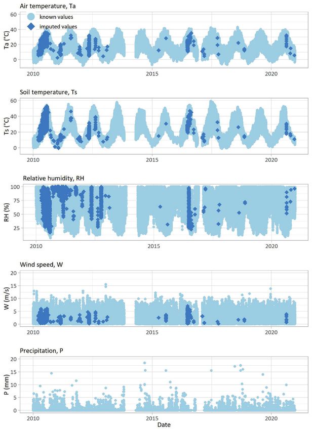
Maria Catarina Paz et al. / REA N. 42 (2021) 202 - 219

1. INTRODUCTION

The dissemination of intensive and super-intensive agriculture is a trend with a worldwide impact. Because
of the production based on mono-culture, and consequent extreme dependence on fertilizers, pesticides
and water irrigation, this type of agriculture can result in unsustainability of production in the medium-long
term, generating (1) loss of soil, biodiversity, and landscape values, (2) water scarcity, and (3) disconnection
from local communities, leading to forced migration of populations and loss of territorial cohesion.
    This type of agriculture has been spreading on the Portuguese landscape in recent decades, intensifying
in the last years. However, Portugal is part of the Mediterranean region, which has been identified by the Eu-
ropean Environment Agency as the most vulnerable of Europe to the negative impacts of climate change on
agriculture (European Environment Agency, 2019). Climate projections for the Mediterranean region predict
an increase of the average air temperature, a precipitation decrease, and an increase in the frequency and
duration of droughts until the end of the 21st century. On the other hand, in Portugal, a considerable part of
the territory has been considered environmentally vulnerable, in what concerns soil, biodiversity, landscape,
and groundwater (Agência Portuguesa do Ambiente, 2016; Instituto Nacional de Estatística, 2019; Direção
Geral de Agricultura e Desenvolvimento Rural, 2021), being therefore protected by legal instruments such as
the European Union (EU) Nitrates directive (1991), the EU Habitats Directive (1992), and the EU Water Frame-
work directive (2000), or conventions, such as the United Nations Ramsar Convention [www.ramsar.org]. At
the same time, populations are very diffusely distributed in the Portuguese territory, especially in the west-
ern and southern zones (Leite, 2014) making it hard to find truly isolated areas where intensive agricultural
farming practices can take place and/or expand without compromising local communities. This way, climate
projections and territorial specificities of natural and social nature make Portugal a place where it is urgent
an open discussion about the sustainability of the actual agricultural development plans and alternatives
including biological, ecological and/or precision farming.
    From a global point of view, and without question, it is vital to maintain food security, both by eradicating
hunger, and therefore securing world peace, and guaranteeing food quality, ensuring healthier and longer
life expectancy. However, the balance between (1) food security, (2) environmental quality and social dignity,                                       203
(3) maintenance of biodiversity, (4) conscious management of the finite resources, and also (5) resilience
facing the impacts of climate change, constitutes the ultimate challenge for contemporary agriculture. This
way, it is convenient to understand which agricultural practices are more adequate to answer this chal-
lenge. In this perspective, ecosystem services, such as natural pest control, pollination, climate regulation,
or carbon sequestration, for instance, may be powerful tools to be incorporated and/or promoted in future
agricultural methodologies but their mechanisms of functioning must be known in order to be used to their
full capacity.
    Natural pest control is an ecosystem service that consists on the reduction of pests by their natural con-
trol agents, which includes predators. Computer models can be used to simulate the interaction between
pests and predators, and therefore to understand how landscape, animals, and agricultural management
are related (Topping et al., 2003; Corral et al., 2011; Ziolkowska et al., 2021). Moreover, these models allow us
to predict how human activity and climate may affect the ecosystem service itself. Complex agro-ecosystem
models are being developed for the olive grove in Portugal. In particular, a model constituted by (1) the
model of one of the key pests of the olive grove, the olive fly Bactrocera oleae (Paz et al., 2021), (2) a ground
spider Haplodrassus rufipes, a generalist predator (Barreira et al., 2020), and (3) the model of a landscape, in
this case representing a section located in Mirandela, NE Portugal, a region mainly devoted to olive produc-
tion, where traditional farming practices are still predominant. These models are simulated and articulated
using the Animal, Landscape and Man Simulation System (ALMaSS) (Topping et al., 2003) through climate
data series and farm management events inputs.
    Whereas farm management events have a non-regular distribution in time, climate data series must have
a regular distribution in time in order for the system to run. However, many times climate data series are not
complete, mostly because of malfunctions of the measuring instruments (Afrifa-Yamoah et al., 2020; Qin et
al, 2021; and references therein), occasional interruptions of automatic stations and/or reorganizations of

 © Editorial Universidad de Sevilla 2021 | Sevilla, España| CC BY-NC-ND 4.0 | e-ISSN: 2340-2776 | doi: https://dx.doi.org/10.12795/rea.2021.i42.10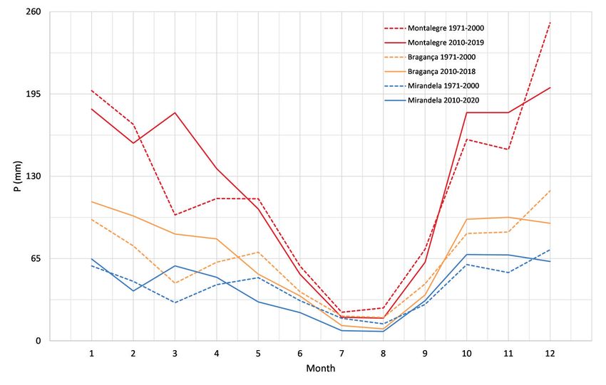
Maria Catarina Paz et al. / REA N. 42 (2021) 202 - 219

networks (Qin et al., 2021; and references therein). This is a common problem that demands the application
of reliable methodologies for filling the gaps. A common way to do this is to replace missing data with rea-
sonable values (Qin et al., 2021; and references therein), a process that, in statistics, is called imputation (Lit-
tle & Rubin, 2002; van Buuren, 2012). In the field of univariate imputation, traditional methods such as mean
imputation, or regression imputation, among others, lacked the utilization of temporal information (Luo et
al., 2018; Qin et al., 2021). Recently, other methods such as model-based ones and software packages are
being developed and evaluated. For instance, Afrifa-Yamoah et al. (2020) has evaluated the performance of
multiple approaches of imputation of missing values in high-resolution univariate climate data series, which
included autoregressive integrated moving average model, structural time series model, both with Kalman
smoothing, and multiple linear regression, verifying low error values and highly acceptable imputations,
which also varied with the climate station location. Qin et al. (2021) developed an imputation method based
on decomposition of time series for univariate climate data with strong spatiotemporal characteristics. Also,
the open source programming language R (R core team, 2020), is being used to complete time series (Dunic
et al., 2021; Engler & Krone, 2021; for instance) and specifically climate data series (Diamond et al., 2021; for
instance,).
    On the other hand, the time step of a measured climate data series may be different from the one needed
for the system to run, which implies the conversion to the desired time step. In the case of the conversion
from hourly data series to daily data series, there is a reduction of temporal resolution and, therefore, a loss
of information in what concerns specific periods of the day. This can be a problem when trying to simulate,
for instance, an animal behaviour that occurs during a specific period of the day. One way to segregate that
specific period would be to create additional daily variables of interest that are calculated using only the
hourly data comprehended in that period. This means that the use of high-resolution temporal climate data
whenever it is possible offers the opportunity to modulate aspects that otherwise would not be perceptible
(Afrifa-Yamoah et al., 2020).
    The objectives of this work are (1) to process climate data series using the open source programming
language R (R core team, 2020), for further application in studies comprising simulations of H. rufipes and
B. oleae in the landscape of Mirandela, (2) to qualitatively verify if the completed data are acceptable to                                           204
feed to the system, and (3) to demonstrate how to create daily variables that represent specific periods of
the day. We expect this paper can be helpful when dealing with similar data and finality. Also, we expect to
encourage the use of models to simulate ecosystem services, contributing to a better knowledge of these
agricultural tools.

2. THEORY

The olive grove, along with human intervention, constitutes an agro-ecosystem where pests and predators
act naturally, ruled by climate variables. The conceptualization of a model for the agro-ecosystem begins
with the knowledge of the functioning of its stakeholders, which is then translated to functions and, fur-
thermore, to computer coding. Climate data needs to be properly prepared to feed these specific computer
simulations.

2.1. The olive grove

The olive grove is a typical Mediterranean crop that occupies a great area in Portugal and has high economic,
social and cultural value. This crop is able to tolerate the low soil water content of semi-arid climates through
a panoply of adaptations developed as response to long periods of water shortage, which may last the entire
spring-summer period (Sofo et al., 2008). Therefore, it is completely adapted to Mediterranean climate.
   Olive oil consumption and demand is increasing worldwide because it is considered beneficial for human
health for its antioxidant properties and balanced fatty acid composition (Brito et al., 2019). Consequently,

  © Editorial Universidad de Sevilla 2021 | Sevilla, España| CC BY-NC-ND 4.0 | e-ISSN: 2340-2776 | doi: https://dx.doi.org/10.12795/rea.2021.i42.10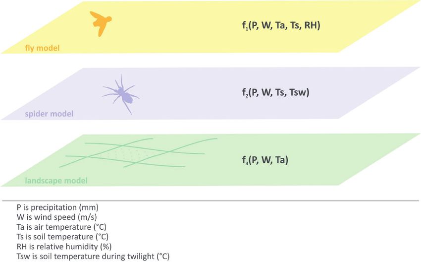
Maria Catarina Paz et al. / REA N. 42 (2021) 202 - 219

natural Mediterranean vegetation and traditional olive grove (with low density of trees per hectare, in dry,
and low or no mechanization at all), are being substituted by high density olive groves (from around 1600 to
3300 trees per hectare, irrigated, and completely mechanized). At this point, it is estimated that high density
olive groves occupy approximately 100000 ha of land in the world, with 41000 located in Spain and 14000
located in Portugal (Roldán et al., 2019). The increase of trees per hectare and its distribution in the field,
along with irrigation, application of fertilizers, modification of practices like harvesting and pruning, and the
preference for specific varieties of olive trees has led to changes and further adaptations of pests to the olive
grove (Roldán et al., 2019) This problem is partly mitigated by the application of pesticides (Paz et al., 2021),
which, by their turn, compromise the safety of olive oil and olives as food, and also the environmental safety
by entering a cycle in the environment that involves the soil, air, aquifers and which duration depends on
many factors such as the type of plant, the type of soil and microorganisms of soil, the climate conditions,
the depth of the groundwater, and the type of pesticide itself (National Pesticide Information Center, 2020).

2.2. Complex agro-ecosystem model

Bactrocera oleae is a dipteran of the family Tephritidae and is considered the key pest of olives in the Medite-
rranean region (Gonçalves, 2011). Life cycle of this insect is closely related to the olive grove seasonal develo-
pment, especially the fruits, where the females place their eggs. Adults first emerge in spring and begin their
activity, feeding on nectar or honeydew (Tzanakakis, 2003). During this period, females usually start laying
eggs on olives that remained on the trees from the previous season. In early summer, high temperatures
inhibit ovarian maturation so flies may disperse through great distances and colonize other groves (Daane
& Johnson, 2010). After this reproductive diapause, females reinitiate laying eggs when the olives reach the
proper development. Eggs evolve to larvae, then pupa, and finally to adults. During summer and early fall,
the development of the fly is completed within the olive, with pupation occurring inside it and adults emer-
ging later in the season. From mid-autumn onwards, an increasing number of larvae fall from the olive fruit
to pupate in the soil, where they overwinter, and emerge as adults in the following spring. Larvae feed upon                                          205
the pulp, causing high economic losses (Gonçalves, 2011). Life cycle of B. oleae greatly depends on climatic
conditions, varying from 30 to 80 days in summer or warmer areas, and up to 130 days in winter or colder
areas. Hot and dry summers result on a delay in the increase of B. oleae populations, while humid and warm
summers lead to early infestations. In continental climate areas, two to three generations are observed per
year while in Mediterranean coastal areas three to four generations are observed per year (Dinis, 2014).
    Haplodrassus rufipes is a predator anthropod of the family Gnaphosidae that inhabits the olive grove and
that can be used to control olive tree pests (Benhadi-Marín, 2019). This is a ground spider that hunts during
the twilight (Benhadi-Marín, J., personal communication) and which main habitat is the soil under stones,
where it finds refuge and breeds (Benhadi-Marín, 2019). The female lays the eggs inside a silken case, plac-
ing it under stones and guarding it until the spiderlings come out. From hatching until becoming adults,
these spiderlings will pass several instars, which are growing stages that are finalized by the replacing of the
cuticle, in a process called moulting. There will be two instars inside the eggsac (Barreira et al., 2020) and it
is thought that about three instars outside the eggsac. Once out of the eggsac, the spiderlings start feeding,
mainly on plant-based food like honeydew or nectar. However, once becoming close to adulthood, this spi-
der becomes a generalist predator, preferring other animals, and bigger ones as it becomes stronger. One
of its preys is B. oleae, which is accessible to this spider when it pupates in the soil.
    Every function of H. rufipes and B. oleae, such as development, mortality, overwintering, movement, and
reproduction depends on climate variables (Barreira et al., 2020; Paz et al., 2021; and references therein). And
so the development of crops (Topping et al., 2019) or the occurrence of extreme climate events. So, a model
that simulates an ecosystem will basically run with climate variables and, consequently, will need climate
data series inputs. This is the case of ALMaSS, a landscape scale system of models that simulates changes in
the landscape structure and in the abundance of animals. ALMaSS combines (1) subpopulation-based sim-
ulation, a modelling technique where agents represent populations of animals, for large populations such

  © Editorial Universidad de Sevilla 2021 | Sevilla, España| CC BY-NC-ND 4.0 | e-ISSN: 2340-2776 | doi: https://dx.doi.org/10.12795/rea.2021.i42.10
Maria Catarina Paz et al. / REA N. 42 (2021) 202 - 219
as B. oleae, and (2) agent-based simulation, where agents represent animals acting in their environment, for
scarce populations such as H. rufipes, with (3) a dynamic landscape simulation that comprises highly detailed
spatial structures and farm management. We can think of this as a system of layers, where each one repre-
sents a model, each depending on a set of climate variables (figure 1).
206
Figure 1. System of layers representing the models, here represented by f1, f2, and f3, of the fly B. oleae, the spider H.
rufipes, and the landscape, respectively. Source: own elaboration.
2.3. Processing of climate data series for simulations in ALMaSS
The time-step used for ALMaSS simulations of H. rufipes and B. oleae in the landscape of Mirandela is 1 day.
In this case, the system needs the following daily climate variables inputs: precipitation (mm), wind speed
(m/s), air temperature (°C), soil temperature (°C), relative humidity (%), and soil temperature during twilight
(°C). Figure 1 specifies the variables that feed to each specific model. This means that for each day of the sim-
ulation, ALMaSS requires one input value for each of these climate variables, or in other words, univariate
(one attribute observed over time), evenly spaced (equal increments between successive data points), nu-
meric (measurable quantities that are expressed as a number) time series (Moritz & Bartz-Beielstein, 2017)
for each variable. Because climate data series are therefore time series, they can be filled, when incomplete,
through imputation, which involves inter-time correlations in the case of univariate time series (Moritz &
Bartz-Beielstein, 2017).
On the other hand, ALMaSS uses a daily time-step which implies that the used climate series are daily data
series. However, there are specific functions of the animals simulated that occur during specific moments of
the day. This way, to segregate the influence of these specific periods of the day, measured data series with
smaller increments between successive data points can be used, for instance hourly values, which then are
converted to daily data series through calculations.
© Editorial Universidad de Sevilla 2021 | Sevilla, España| CC BY-NC-ND 4.0 | e-ISSN: 2340-2776 | doi: https://dx.doi.org/10.12795/rea.2021.i42.10Maria Catarina Paz et al. / REA N. 42 (2021) 202 - 219
3. METHODOLOGY
3.1. Study area
The study area (figure 2) is located in Northeast Portugal, in the region of Trás-os-Montes, in a sub region
called Terra Quente (which translation to English is Warm Land), because of its special climate. In fact, ac-
cording to the Köppen-Geiger classification (Instituto Português do Mar e da Atmosfera, 2021a), in Terra
Quente climate is temperate with rainy winters and hot and dry summers (Csa), as result of the orography
of the region. This determines typical Mediterranean vegetation and agriculture (Associação de Municípios
da Terra Quente Transmontana, 2021). Land cover consists mainly of a mosaic of small parcels (about 2 to 3
ha) of olive groves, vineyards, almond orchards, and semi-natural heaths with Quercus rotundifolia and high
herbaceous strata. This landscape structure allows high biodiversity and, from the olive production point of
view, it is considered much more sustainable than bigger parcels of olive tree mono-culture. In fact, the mo-
saic landscape contributes to the reduction of pest migration and also promotes the existence of predators
to those pests (Villa, 2020a, 2020b).
207
Figure 2. Location of the study area and the Mirandela climate station. Source: Google Earth.
© Editorial Universidad de Sevilla 2021 | Sevilla, España| CC BY-NC-ND 4.0 | e-ISSN: 2340-2776 | doi: https://dx.doi.org/10.12795/rea.2021.i42.10Maria Catarina Paz et al. / REA N. 42 (2021) 202 - 219
3.2. Climate data series of Mirandela
Climate data series were measured hourly, from 2010 to 2020, at the Mirandela climate station (Figure 2),
located at an altitude of 250 m. This station is part of the network of climate stations of Instituto do Mar e da
Atmosfera (IPMA), the Portuguese state agency for climate. Air temperature was measured at 1.5 m above
the soil, and soil temperature was measured at a depth of 0.05 m.
The raw data contained time series, for each variable, of length 96360. However, a considerable amount
of missing values was present for each measured variable as summarized in table 1. Particularly, February
and March 2014 were missing, representing the biggest gap in the raw data. Processing of data to create
complete daily data series was performed using R language (R Core team, 2020), and followed the sequence
displayed in figure 3. Each variable was treated separately. Most variables, such as air temperature and soil
temperature (and even relative humidity and wind speed, although not so strongly), present daily and yearly
seasonality. Precipitation does not fall in this category so it was treated using a slightly different approach.
For completing the task of imputation, we have used some of the functions of the R package imputeTS, a
package built specifically for univariate time series imputation of missing values (Moritz & Bartz-Beielstein,
2017). This package uses a process for imputation that starts by analysing the distribution of the missing
values, then performs the imputation based on one of the available algorithms, and finally visualizes the
imputations in the time series (Moritz & Bartz-Beielstein, 2017).
Table 1. Missing values in the time series of climate variables recorded between 2010 and 2020 at Mirandela climate station.
Number of missing Percentage of Most frequent gap
Variable Number of gaps Longest gap size
values missing values size
Ta 9160 10% 77 1 4285
Ts 9172 10% 88 1 4285
RH 9818 10% 182 1 4285 208
W 9308 10% 72 1 4285
P 11065 12% 79 1 4286
Ta is air temperature (°C)
Ts is soil temperature (°C)
RH is relative humidity (%)
W is wind speed (m/s)
P is precipitation (mm)
3.3. Imputation of missing data and conversion of hourly to daily data
Given the seasonality of the time series, we have used the function na seadec() from the imputTS package,
using the algorithm Weighted Moving Average. na_seadec() estimates seasonality frequency automatically
from data and performs the imputation automatically. However, it works poorly for longer gap sizes. There-
fore, we have established a threshold of 500 consecutive missing values to be automatically completed by
this function. For the remaining missing values, we aggregated air temperature by daily mean, for all days
with no missing values. Otherwise, we assumed the days would have no value (NA). After that stage, we have
done imputation of those missing values as the mean of all the non-missing values for the same day in the
year for all the years present in the data. For soil temperature time series we have used the same approach
as for air temperature.
In the case of relative humidity, the same function we used for completing air temperature and soil tem-
perature does not provide such good results. Therefore, we used na_seasplit() instead. This function splits
time series into seasons and afterwards performs imputation separately for each of the resulting time series
© Editorial Universidad de Sevilla 2021 | Sevilla, España| CC BY-NC-ND 4.0 | e-ISSN: 2340-2776 | doi: https://dx.doi.org/10.12795/rea.2021.i42.10Maria Catarina Paz et al. / REA N. 42 (2021) 202 - 219
datasets. There are several algorithms that can be used along this function. We have chosen the Weighted
Moving Average. As we have done for the previous time series air temperature and soil temperature, we
have established a threshold of 500 consecutive missing values to be automatically completed by this func-
tion. After this stage, we aggregated data by daily means, attributing NA for every day for which there would
be at least one missing value. We have then completed the daily means time series using the same strategy
as for air temperature and soil temperature. For the wind speed, the approach used was exactly the same as
the one used for completing relative humidity.
For precipitation we took a different approach as this variable is known to have a more stochastic behav-
iour. To try to remove the noise and be able to use some pattern that we can observe along the year when
looking at daily precipitation, instead of completing the hourly data, we will assume a day as a missing day if
in it there is at least one missing hourly value. Otherwise, we will sum up all hourly values. Still, this produces
a time series with missing data. Therefore, we completed the missing values as the mean of all the non-miss-
ing values for the same day in the year for all the years present in the data.
We didn’t use data from the two IPMA nearby stations, Montalegre and Bragança, because they were
located in areas with a different climate. In fact, and as explained above, Mirandela climate station is located
in a sub region where orography determines a climate different from the rest of the region, Csa, and Csb
respectively, according to Köppen-Geiger classification (Instituto Português do Mar e da Atmosfera, 2021).
Daily air temperature, soil temperature, relative humidity and wind speed were obtained calculating the
mean of the 24 hourly measures of each day, whereas daily precipitation was obtained calculating the sum
of the 24 hourly measures of each day.
209
Figure 3. Sequence of the processing of climate data using R language. Source: Own elaboration.
© Editorial Universidad de Sevilla 2021 | Sevilla, España| CC BY-NC-ND 4.0 | e-ISSN: 2340-2776 | doi: https://dx.doi.org/10.12795/rea.2021.i42.10Maria Catarina Paz et al. / REA N. 42 (2021) 202 - 219
3.4. Calculation of soil temperature during twilight
We defined the twilight period as the period between sunset and the end of astronomical twilight, that is,
when the Sun is 18° below the horizon. From [http://www.cavu.info/sunset.html], we retrieved the times of
these two moments during the year, for the location of the Mirandela climate station. Based on these data
we built a table containing nine columns: month, day, sunset, end of astronomical twilight, duration (the dif-
ference between the two), the hour of sunset, the minute of sunset, the hour of end of astronomical twilight,
and the minute of end of astronomical twilight.
Daily soil temperature during twilight was calculated as the weighted mean of hourly soil temperature
measurements registered during the twilight period. To better explain it, we present an example. If in day
N sunset starts at 17:12 and ends at 18:52, we will retrieve hourly Ts at 17:00 and at 18:00 (Ts17 and Ts18) and
for day N we will have that soil temperature during twilight (Tsw) is given by:
Note that in case there is some missing value in hourly soil temperature, we will assume soil temperature
during twilight is simply the soil temperature daily mean.
3.5. A
cceptability of the calculated daily data series of air temperature, relative humidity, wind speed,
and precipitation
To infer if the data series obtained with our methodology were acceptable for using in the ALMaSS simula-
tion, we calculated the monthly inter-annual means for the period 2010–2020, using the same method as
the one used for calculating the climate normals (World Meteorological Organization, 2017), and compared 210
the obtained annual pattern with that of the climate normals for the period 1971–2000 registered at the
Mirandela climate station (Instituto Português do Mar e da Atmosfera, 2021). The monthly inter-annual
means for the period 2010–2020 were calculated using the converted daily data series of air temperature,
relative humidity, wind speed, and precipitation. For air temperature, relative humidity, and wind speed, we
converted daily to monthly data calculating the mean of the daily values of each month, and then grouped
the monthly values of each year per month, and calculated the mean (World Meteorological Organization,
2017). For precipitation we converted daily data to monthly data calculating the sum of the values of each
month, and then grouped the monthly values of each year per month, and calculated the mean (World Me-
teorological Organization, 2017).
4. RESULTS AND DISCUSSION
4.1. Completed hourly climate data series
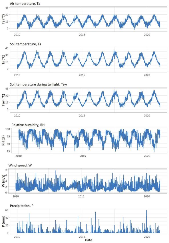
Figure 4 displays the hourly known values of air temperature, soil temperature, relative humidity, wind
speed and precipitation measured between 2010 and 2020 at Mirandela climate station. It is evident the
large gap comprising February and March 2014. In these climate data series, hourly air temperature ranges
between –8.00 °C and 43.00 °C, with a mean of 15.16 °C; hourly soil temperature ranges between –1.00 °C
and 59.30 °C, with a mean of 19.07 °C; hourly relative humidity ranges between 7 % and 100 %, with a mean
of 70.64 %; hourly wind speed ranges between 0 m/s and 15.50 m/s, with a mean of 1.93 m/s; and hourly
precipitation ranges between 0 mm and 18.50 mm, with a mean of 0.06 mm.
© Editorial Universidad de Sevilla 2021 | Sevilla, España| CC BY-NC-ND 4.0 | e-ISSN: 2340-2776 | doi: https://dx.doi.org/10.12795/rea.2021.i42.10Maria Catarina Paz et al. / REA N. 42 (2021) 202 - 219
211
Figure 4. Known hourly values of air temperature, soil temperature, relative humidity, wind speed and precipitation,
and imputed hourly values of air temperature, soil temperature, relative humidity and wind speed using function
na_seadec() , for the climate data series recorded between 2010 and 2020 at Mirandela climate station. Note that gap
sizes larger than 500 consecutive values were not filled in. Source: Own elaboration.
© Editorial Universidad de Sevilla 2021 | Sevilla, España| CC BY-NC-ND 4.0 | e-ISSN: 2340-2776 | doi: https://dx.doi.org/10.12795/rea.2021.i42.10Maria Catarina Paz et al. / REA N. 42 (2021) 202 - 219 We can see the clear periodic variability of air temperature and soil temperature, which translates in not only seasonal patterns but also daily patterns. Relative humidity also seems to exhibit some seasonal peri- odic variability. Air temperature and soil temperature show peaks in warm seasons and valleys in cold sea- son, relating roughly to relative humidity, which shows valleys when air and soil temperature show peaks. Wind speed and precipitation do not reveal such clear patterns at this point. Figure 4 also displays the hourly imputed values of air temperature, soil temperature, relative humidity and wind speed in the measured time series, with imputations done when gap sizes were not larger than 500 consecutive values. We can see that the imputed values are well blended in the four data patterns, cre- ating time series that are acceptable to proceed in the processing towards the conversion into daily values of air temperature, soil temperature, relative humidity and wind speed, and also to calculate daily values of soil temperature during twilight. Imputed values of hourly precipitation are not shown here because, as explained in the previous section, the methodology we used excluded days where there was at least one missing hourly value, and so, for interpretation purposes, we only show the measured hourly values of pre- cipitation. 4.2. Daily climate data series Figure 5 displays the calculated daily time series of air temperature, soil temperature, soil temperature dur- ing twilight, relative humidity, wind speed, and precipitation, for the period 2010–2020 at Mirandela climate station. In these data series, daily air temperature ranges between –2.55 °C and 32.35 °C, with a mean of 14.83 °C; daily soil temperature ranges between 0.35 °C and 40.57 °C, with a mean of 18.63 °C; daily soil temperature during twilight ranges between 0.82 °C and 41.71 °C, with a mean of 20.48 °C; daily relative humidity ranges between 22.04 % and 100 %, with a mean of 71.42 %; daily wind speed ranges between 0.10 m/s and 7.60 m/s, with a mean of 1.92 m/s; and daily precipitation ranges between 0 mm and 59.00 mm, with a mean of 1.40 mm. With hourly data converted into daily data, we can better observe the periodic variability of the time 212 series. In the case of daily air temperature, soil temperature, and soil temperature during twilight, the sea- sonal variability is revealed through a pattern formed by peaks – warm seasons – and valleys – cold seasons (National Weather Service, 2021). Also, we can see that the fluctuations of daily air temperature, soil tem- perature, and soil temperature during twilight during cold seasons seem to be greater than the fluctuations during warm seasons. Seasonal variability of daily relative humidity, wind speed and precipitation also exhibit seasonal patterns, although with different shapes than the daily temperatures. Note that the valleys in daily relative humidity occur when there are peaks in the daily temperatures and the peaks in daily relative humidity occur when there are valleys in the temperatures. Relative to inter-annual variability, we can see that there are variations in all data series. Precipitation shows the most evident inter-annual variability, with peaks of different magnitude occurring in different years, which also happens for the rest of the data series but not so visibly. Daily relative humidity and wind speed data series show a slightly different change in the inter-annual pattern in the February 2014–March 2014 period. 4.3. Acceptability of processed climate data series Figure 6 shows the annual patterns of the monthly inter-annual means for the period 2010–2020 and the climate normals for the period 1971–2000 registered at the Mirandela climate station (Instituto Português do Mar e da Atmosfera, 2021a). © Editorial Universidad de Sevilla 2021 | Sevilla, España| CC BY-NC-ND 4.0 | e-ISSN: 2340-2776 | doi: https://dx.doi.org/10.12795/rea.2021.i42.10
Maria Catarina Paz et al. / REA N. 42 (2021) 202 - 219

                                                                                                                                                      213

Figure 5. Calculated daily time series of air temperature, soil temperature, soil temperature during twilight, relative hu-
midity, wind speed, and precipitation, for the period 2010–2020 at Mirandela climate station. Source: Own elaboration.

  © Editorial Universidad de Sevilla 2021 | Sevilla, España| CC BY-NC-ND 4.0 | e-ISSN: 2340-2776 | doi: https://dx.doi.org/10.12795/rea.2021.i42.10
Maria Catarina Paz et al. / REA N. 42 (2021) 202 - 219
214
Figure 6. Monthly inter-annual means calculated for the period 2010–2020 and the climate normals for the period
1971-2000 registered at the Mirandela climate station (Instituto Português do Mar e da Atmosfera, 2021a). Source: Own
elaboration for the monthly inter-annual means; IPMA for the climate normals.
We can see that the annual patterns of mean air temperature for the two periods are almost coincident. We
believe soil temperature and soil temperature during twilight, although not present in this analysis, would have
similar results to air temperature, because of the evident periodicity of the hourly data series, which allows us
© Editorial Universidad de Sevilla 2021 | Sevilla, España| CC BY-NC-ND 4.0 | e-ISSN: 2340-2776 | doi: https://dx.doi.org/10.12795/rea.2021.i42.10Maria Catarina Paz et al. / REA N. 42 (2021) 202 - 219
to complete the series efficiently. Mean relative humidity patterns are also very similar, with exception of the
first four months of the year, in which the 2010–2020 period shows lower values. Mean wind speed patterns
are similar, with the 2010–2020 period showing slightly lower values especially during the cold season. Also
mean wind speed in the 2010–2020 period shows a peak in March, while the climate normal shows a peak in
April. Mean precipitation patterns are the least coincident, with the 2010–2020 period showing higher values
than the climate normal from September to April approximately, with a valley in February and a peak in March.
To investigate if this disconnection was related to the inefficiency of our methodology or it they were a
result of climate evolution, we compared the monthly inter-annual mean precipitation and climate normals
measured at Mirandela (already shown in Figure 6) with those measured at the Montalegre and Bragança cli-
mate stations (Instituto Português do Mar e da Atmosfera, 2021b), located in Trás-os-Montes, approximately at
60 km northwest and 50 km northeast, respectively. Figure 7 shows this comparison. We can see that the be-
haviour of the pattern for the period 2010–2019 of Montalegre in February and March is similar to the pattern
of Mirandela for the period 2010–2020, both being disconnected from the respective climate normal in these
months. Also, the behaviour of the pattern for the period 2010–2018 of Bragança in December is similar to the
pattern of Mirandela for the period 2010–2020, both being disconnected from the respective climate normal
in this month. This suggests that the disconnection between the climate patterns obtained with our methodol-
ogy and the climate normals, may be related to a climate evolution, rather than to an ineffective methodology
In fact, in what concerns air temperature and precipitation, our methodology produced data series, that,
for the period 2010-2020 (figure 6), show higher air temperature throughout the year, especially from March
to September, and a shorter and wetter rainy season. This is in accord with the global and regional climate
projections for the Portuguese territory, which predict an increase in air temperature, and in precipitation
during a shorter season, and are expected to have more impact in summer and autumn (Miranda et al.,
2002). Therefore, we consider all the processed time series good enough for the system to run.
215
Figure 7. Monthly inter-annual means calculated for the period 2010–2020 and the climate normals for the period
1971–2000 registered at the Mirandela climate station (Instituto Português do Mar e da Atmosfera, 2021a), and at Mon-
talegre and Bragança climate stations (Instituto Português do Mar e da Atmosfera, 2021b). Source: Own elaboration for
the monthly inter-annual means; IPMA for the climate normals.
© Editorial Universidad de Sevilla 2021 | Sevilla, España| CC BY-NC-ND 4.0 | e-ISSN: 2340-2776 | doi: https://dx.doi.org/10.12795/rea.2021.i42.10Maria Catarina Paz et al. / REA N. 42 (2021) 202 - 219
4.4. Expression of periods of the day through a daily value – the case of soil temperature during twilight
Figure 8 shows an example of the daily data series of soil temperature and soil temperature during twilight
for one year. We chose the year 2011, during which data for animal abundance was collected. We can verify
that soil temperature during twilight is in general higher than soil temperature. The use of the more gen-
eral soil temperature variable instead of the specific soil temperature during twilight variable, would lead
to incorrect results from the simulation of the spider movement, which is known to happen during the twi-
light period in real life (Benhadi-Marín, J., personal communication). This way, it was possible to modulate
an aspect that otherwise would not have impact on the simulations, meaning that we can detect and filter
important attributes when using high-resolution temporal climate data, as suggested by Afrifa-Yamoah et al.
(2020). Therefore, our methodology allowed to segregate the temperature during twilight as a daily value,
reducing the error associated with the use of a daily climate value to express functions that occur during
specific periods of the day, but respecting the time step of the system.
216
Figure 8. Daily data series of soil temperature and soil temperature during twilight for the year 2011, calculated from
the hourly data series measured at Mirandela climate station. Source: Own elaboration.
These results may also give some more information to understand why the spider prefers this specific
period of the day to hunt and move.
5. CONCLUSIONS
The applied methodology allowed us to produce well blended imputations, creating acceptable completed
hourly time series and posteriorly, acceptable daily data series for the system to run. Our methodology also
allowed to segregate the temperature during twilight as a daily value. This enables to reduce the error asso-
ciated with the use of a daily climate value to express functions that occur during specific periods of the day.
In fact, we verified that mean soil temperature during twilight is higher than daily mean soil temperature.
This way, it is convenient that the system runs with the variable soil temperature during twilight to emulate
the spider hunting during the twilight in real life, instead of the more general variable soil temperature.
The specific methodology proposed in this paper will be further developed to process climate data for
ALMaSS simulations of other pests and predators of the olive grove in the Mirandela study site. As ALMaSS
© Editorial Universidad de Sevilla 2021 | Sevilla, España| CC BY-NC-ND 4.0 | e-ISSN: 2340-2776 | doi: https://dx.doi.org/10.12795/rea.2021.i42.10Maria Catarina Paz et al. / REA N. 42 (2021) 202 - 219
is being implemented in other study sites including olive groves across Europe, the proposed methodology
can also be used wherever there is available hourly climate data. We also intend to test our methodology
with a more formal approach in the future.
With this work, we expect to have contributed with an expedite methodology and ideas for climate data
series processing and further use in agro-ecosystem modelling. This way, we also wish to contribute to a
better understanding of the mechanisms behind the functioning of ecosystems services, in particular the
functioning of natural pest control, which is an important alternative to pesticide application as one of the
answers to the great challenge of contemporary agriculture: to produce healthy and enough food, maintain-
ing environmental quality and social dignity, conserving biodiversity, consciously managing finite resources,
while adapting to climate change.
Funding
This work was funded by Fundação para a Ciência e a Tecnologia through project PTDC/ASP-PLA/30003/2017
- OLIVESIM - Managing ecosystem services in olive groves using advanced landscape agent-based models.
R.B. acknowledges support from the National Funding from FCT – Fundação para a Ciência e a Tecnologia,
under the project UIDB/04561/2020.
Acknowledgements
The authors are grateful to Instituto Português do Mar e da Atmosfera for the hourly climate data measured
at the Mirandela climate station.
Responsible reporting and conflict of interest 217
The authors declare no conflict of interest. M.C.P. and R.B. processed the climate data series. R.B. and M.C.P.
developed the methodology. M.C.P. and R.B. wrote the manuscript and prepared the visualisation. S.A.P.S.
revised the manuscript. S.A.P.S. and R.B. acquired the funding.
REFERENCES
Afrifa-Yamoah, E., Mueller, U., Taylor, S. & Fisher, A. (2020). Missing data imputation of high‐resolution temporal climate
time series data. Meteorological Applications, 27. https://doi.org/10.1002/met.1873.
Agência Portuguesa do Ambiente (2016). Poluição Provocada Por Nitratos De Origem Agrícola – Diretiva 91/676/CEE, de 12
de dezembro – Relatório 2012-2015.
Associação de Municípios da Terra Quente Transmontana (2021, 15 May). Caracterização. https://www.amtqt.pt/pages/298
Barreira, R., Paz, M.C., Amaro, L., Sousa, J.P., Benhadi-Marín, J., Rasko, M., Alves da Silva, A., Alves, J., Chuhutin, A., Top-
ping, C.J. & Santos S.A.P. (2020). Developing an Agent-Based Model for Haplodrassus rufipes (Araneae: Gnaphosidae),
a Generalist Predator Species of Olive Tree Pests: Conceptual Model Outline. https://doi.org/10.3390/IECPS2020-08745
Benhadi-Marín, J. (2019). Diversity Patterns of Araneae along a Gradient of Farming Practices in Olive Groves: Linking Landsca-
pe Pattern, Management Practices, and Species Interactions. [Ph.D. Thesis, University of Coimbra]. http://hdl.handle.
net/10316/87551
Brito C., Dinis, L.-T., Moutinho-Pereira, J. & Correia, C.M. (2019). Drought stress effects and olive tree acclimation under a
changing climate. Plants, 8, 232. https://doi.org/10.3390/plants8070232
Corral, J. & Calegari, D. (2011). Towards an Agent-Based Methodology for Developing Agro-Ecosystem Simulations. In G.
Barthe, A. Pardo & G. Schneider (eds.) SEFM 2011: Software Engineering and Formal Methods (pp 431-446). Springer.
https://doi.org/10.1007/978-3-642-24690-6_30
© Editorial Universidad de Sevilla 2021 | Sevilla, España| CC BY-NC-ND 4.0 | e-ISSN: 2340-2776 | doi: https://dx.doi.org/10.12795/rea.2021.i42.10Maria Catarina Paz et al. / REA N. 42 (2021) 202 - 219
Daane, K. M. & Johnson, M. W. (2010). Olive fruit fly: managing an ancient pest in modern times. Annual Review of Ento-
mology, 55, 155–169. https://doi.org/10.1146/annurev.ento.54.110807.090553
Diamond, J., Moatar, F., Cohen, M., Poirel, A., Martinet, C., Maire, A. & Pinay, G. (2021). Metabolic regime shifts and ecosys-
tem state changes are decoupled in a large river. Limnology and Oceanography. https://doi.org/10.1002/lno.11789.
Direção Geral de Agricultura e Desenvolvimento Rural. (2021, 15 May). Zonas Vulneráveis. https://www.dgadr.gov.pt/rec-
hid/diretiva-nitratos/zonas-vulneraveis
Dinis, A.M. (2014). Role of edaphic arthropods on the biological control of the olive fruit fly (Bactrocera oleae). [Ph.D. Thesis,
Polytechnic Institute of Bragança]. http://hdl.handle.net/10198/11593
Dunic, J., Brown, C., Connolly, R., Turschwell, M. & Côté, I. (2021). Long‐term declines and recovery of meadow area across
the world’s seagrass bioregions. Global Change Biology. https://doi.org/10.1111/gcb.15684.
Engler, M. & Krone, O. (2021). Movement patterns of the White‐tailed Sea Eagle (Haliaeetus albicilla): post‐fledging beha-
viour, natal dispersal onset and the role of the natal environment. Ibis. https://doi.org/10.1111/ibi.12967.
European Environment Agency (2019). Climate change adaptation in the agriculture sector in Europe. EEA Report No 4/2019.
https://www.eea.europa.eu/publications/cc-adaptation-agriculture.
Gonçalves, M.F. (2011). Control of the olive fly, Bactrocera oleae (Rossi), in the context of a sustainable production of olives.
[Ph.D. Thesis, University of Trás-os-Montes and Alto Douro].
Habitats Directive. (1992). Council Directive 92/43/EEC of 21 May 1992 on the conservation of natural habitats and of wild
fauna and flora. Official Journal of the European Communities, 22/07/1992, L 206, 0007–0050.
Instituto Nacional de Estatística. (2019). Estatísticas do Ambiente.
Instituto Português do Mar e da Atmosfera. (2021a, 15 May). Normais Climatológicas. https://www.ipma.pt/pt/oclima/
normais.clima/
Instituto Português do Mar e da Atmosfera. (2021b, 05 July). Séries Longas. https://www.ipma.pt/pt/oclima/series.longas/
Leite, I. (2021, 07 June). Rede urbana e sistema urbano. https://www.slideshare.net/seculoXXI/rede-e-sistema-urba-
nos-em-portugal2
Little, R.J.A. & Rubin, D.B. (2002). Statistical analysis with missing data, 2nd ed. Wiley, Hoboken. https://doi.
org/10.1002/9781119013563
Luo, Y., Cai, X., Zhang, Y., Xu, J. & Yuan, X. (2018). Multivariate time series imputation with generative adversarial networks. 218
32nd Conference on Neural Information Processing Systems. Montréal, Canada.
Miranda, P., Coelho, M.F., Tomé, A., Valente, M., Carvalho, A., Pires, C., Pires, H.O., Pires, V. & Ramalho, C. (2002). 20th
Century Portuguese Climate and Climate Scenarios. In F.D. Santos, K. Forbes, & R. Moita (eds.) Climate Change in
Portugal: Scenarios, Impacts and Adaptation Measures (SIAM Project) (p. 23-83). Gradiva.
Moritz, S. & Bartz-Beielstein, T. (2017) imputeTS: Time series missing value imputation in R. The R Journal, 9:1, 207–2018.
https://doi.org/10.32614/RJ-2017-009
National Pesticide Information Center (2020) Pesticide movement in the environment. http://npic.orst.edu/outreach/mo-
vement-infographic.png
National Weather Service. (2021, 07 July). Climate Time Series: Seasonal Variability. https://training.weather.gov/pds/clima-
te/pcu2/statistics/Stats/part1/CTS_SeaVar.htm
Nitrates Directive. (1991). Directive 91/676/EEC of 12 December 1991 concerning the protection of waters against pollu-
tion caused by nitrates from agricultural sources. Official Journal of the European Communities, 31/12/1991, L375, 1–13.
Paz, M.C., Santos S.A.P., Barreira, R., Rasko, Duan, X., Alves, J., Alves da Silva, A., Mina, R., Topping, C.J. & Sousa, J.P. (2021)
Developing a subpopulation-based model for the olive fruit fly Bactrocera oleae (Diptera: Tephritidae): conceptual
model outline. The 1st International Electronic Conference on Agronomy. https://doi.org/10.3390/IECAG2021-09680
Qin, Y., Ren, G., Zhang, P. Wu, L. & Wen, K. (2021). An imputation method for the climatic data with strong seasonality and
spatial correlation. Theoretical and Applied Climatology, 144. https://doi.org/10.1007/s00704-021-03537-9.
Sofo, A., Manfreda, S., Fiorentino, M., Dichio, B. & Xiloyannis, C. (2008) The olive tree: a paradigm for drought tolerance
in Mediterranean climates. Hydrology and Earth System Sciences, 12, 293–301. https://doi.org/10.5194/hess-12-
293-2008
Topping, C.J., Hansen, T.S., Jensen, T.S., Jepsen, J.U., Nikolajsen, F. & Odderskær, P. (2003). ALMaSS, an agent-based model
for animals in temperate European landscapes. Ecological Modelling, 167, 65–82. https://doi.org/10.1016/S0304-
3800(03)00173-X
© Editorial Universidad de Sevilla 2021 | Sevilla, España| CC BY-NC-ND 4.0 | e-ISSN: 2340-2776 | doi: https://dx.doi.org/10.12795/rea.2021.i42.10Maria Catarina Paz et al. / REA N. 42 (2021) 202 - 219
Topping, C.J., Dalby, L. & Valdez, J.W. (2019). Landscape-scale simulations as a tool in multi-criteria decision making for
agri-environment schemes. Agricultural Systems, 176, https://doi.org/10.1016/j.agsy.2019.102671.
R Core Team. (2020). R: A language and environment for statistical computing. R Foundation for Statistical Computing,
Vienna. https://www.R-project.org/.
Roldán, R.A., Brito, A. & Tinelli, F. (2019) Pests and diseases of the olive tree, EIP-AGRI Focus Group. European Comission. ht-
tps://ec.europa.eu/eip/agriculture/sites/default/files/fg33_mp_effectsofintensification_2019_en.pdf
Tzanakakis, M.E. (2003). Seasonal development and dormancy of insects and mites feeding on olive: a review. Nether-
lands Journal of Zoology, 52, 87–224. http://dx.doi.org/10.1163/156854203764817670
Van Buuren, S. (2012). Flexible imputation of missing data, 2nd ed. Chapman and Hall/CRC, Boca Raton. https://doi.
org/10.1201/b11826
Villa, M., Santos, S.A.P., Aguiar, C. & Pereira, J. (2020a). Plants Biodiversity in Olive Orchards and Surrounding Landscapes
from a Conservation Biological Control Approach. The 1st International Electronic Conference on Agronomy. https://
doi.org/10.3390/IECPS2020-08604.
Villa, M., Santos, S.A.P., Pascual, S. & Pereira, J. (2020b). Do non-crop areas and landscape structure influence dispersal
and population densities of male olive moth? Bulletin of Entomological Research, 111, 1–9. https://doi.org/10.1017/
S0007485320000310.
Water Framework Directive (2000). Directive 2000/60/EC of the European Parliament and of the Council of 23 October
2000 establishing a framework for community action in the field of water policy. Official Journal of the European
Communities, 22/12/2000, L 327, 0001–0073.
World Meteorological Organization (2017). WMO Guidelines on the Calculation of Climate Normals. WMO-No. 1203. https://
library.wmo.int/doc_num.php?explnum_id=4166
Ziółkowska, E., Topping, C.J., Bednarska, A.J. & Laskowski, R. (2021). Supporting non-target arthropods in agroecosys-
tems: Modelling effects of insecticides and landscape structure on carabids in agricultural landscapes. Science of
the Total Environment, 774, 145746. https://doi.org/10.1016/j.scitotenv.2021.145746.
219
© Editorial Universidad de Sevilla 2021 | Sevilla, España| CC BY-NC-ND 4.0 | e-ISSN: 2340-2776 | doi: https://dx.doi.org/10.12795/rea.2021.i42.10You can also read