Occlusion-aware 3D Morphable Models and an Illumination Prior for Face Image Analysis - gravis
←
→
Page content transcription
If your browser does not render page correctly, please read the page content below
Occlusion-aware 3D Morphable Models and an
Illumination Prior for Face Image Analysis
Bernhard Egger · Sandro Schönborn · Andreas Schneider · Adam
Kortylewski · Andreas Morel-Forster · Clemens Blumer · Thomas
Vetter

Abstract Faces in natural images are often occluded          1 Introduction
by a variety of objects. We propose a fully automated,
probabilistic and occlusion-aware 3D Morphable Face          Face image analysis is a major field in computer vision.
Model adaptation framework following an Analysis-by-         We focus on 3D reconstruction of a face given a sin-
Synthesis setup. The key idea is to segment the image        gle still image under occlusions. Since the problem of
into regions explained by separate models. Our frame-        reconstructing a 3D shape from a single 2D image is in-
work includes a 3D Morphable Face Model, a prototype-        herently ill-posed, a strong object prior is required. Our
based beard model and a simple model for occlusions          approach builds on the Analysis-by-Synthesis strategy.
and background regions. The segmentation and all the         We extend the approach by an integrated segmentation
model parameters have to be inferred from the single         into face, beard and non-face to handle occlusions.
target image. Face model adaptation and segmentation             We work with a 3D Morphable Face Model (3DMM)
are solved jointly using an expectation–maximization-        as originally proposed by Blanz and Vetter (1999) rep-
like procedure. During the E-step, we update the seg-        resenting the face by shape and color parameters. With
mentation and in the M-step the face model parame-           illumination and rendering parameters we can synthe-
ters are updated. For face model adaptation we apply a       size facial images. We adapt all parameters to render
stochastic sampling strategy based on the Metropolis-        an image which is as similar as possible to the target.
Hastings algorithm. For segmentation, we apply Loopy         This process is called fitting.
Belief Propagation for inference in a Markov random              Most “in the wild” face images depict occluders
field. Illumination estimation is critical for occlusion     like glasses, hands, facial hair, microphones and various
handling. Our combined segmentation and model adap-          other things (see Köstinger et al (2011)). Such occlu-
tation needs a proper initialization of the illumination     sions are a challenge in an Analysis-by-Synthesis setting
parameters. We propose a RANSAC-based robust illu-           - the fitting procedure of 3DMMs is misled by them. Oc-
mination estimation technique. By applying this method       clusions make the face model either drift away, or the
to a large face image database we obtain a first empir-      shape and color parameters are distorted because the
ical distribution of real-world illumination conditions.     face model adapts to those occlusions. Standard meth-
The obtained empirical distribution is made publicly         ods like e.g. robust error measures are not sufficient for
available and can be used as prior in probabilistic frame-   generative face image analysis since they tend to ex-
works, for regularization or to synthesize data for deep     clude important details like the eyes, eyebrows or mouth
learning methods.                                            region which are more difficult to explain by the face
                                                             model (see Figure 2). At the same time, it is impossi-
                                                             ble to detect occlusions without strong prior knowledge.
                                                             The challenge of occlusion-aware model adaptation is to
                                                             explain as much as possible by the face model and only
                                                             Department of Mathematics and Computer Science
                                                             University of Basel
                                                             Basel Switzerland
                                                             E-mail: bernhard.egger@unibas.ch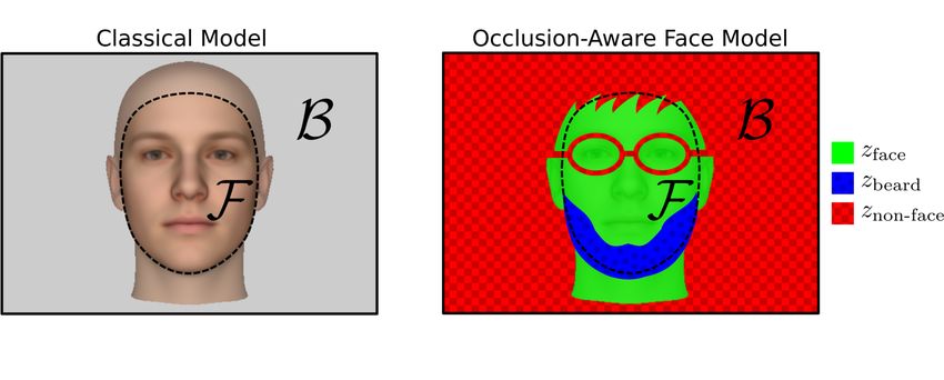
2                                                                                                    Bernhard Egger et al.

Fig. 1: Illumination dominates facial appearance. We indicate the RMS-distance in color space of different render-
ings against a target rendering (a). We rendered the same target under new illumination conditions (b-d), compared
to other changes (e-g). We present a frontal illumination (b), an illumination from the side (c) and a real-world
illumination (d). For comparison, we rendered the original face (a) under the original illumination conditions with
strong changes in pose (e), shape (f) and texture (g). All those changes (e-g) are influencing the distance to the
target image less than changes in illumination (b-d). The shown RMS distances caused by illumination are on
average 50% higher than those caused by changing other parameters.

        (a) target         (b) z , trimmed 70%         (c) z , proposed      (d) θ, trimmed 70%       (e) θ, proposed

Fig. 2: The effect of illumination on a standard robust technique. (a) depicts the target image from the AR face
database by Martinez and Benavente (1998) under homogeneous and inhomogeneous illumination. (b) and (d)
are showing the segmentation and fitting result using a trimmed evaluator as described in Egger et al (2016)
(considering only the best matching 70% of the pixels). (c) and (e) depicts the segmentation and fitting result of
the proposed method. Whilst the segmentation using the trimmed version succeeds only with homogeneous frontal
illumination and fails with illumination from the side, our approach is illumination-invariant and succeeds in both
cases for segmentation and fitting.

exclude non-face pixels. At the same time, it should not         by a darker illumination. The beard region tends to mis-
tend to include occlusions or strong outliers.                   lead illumination estimation and the model adaptation.
    In the proposed framework we distinguish between             Another challenge with beards is that they share their
occlusions that are specific for faces like beards or glasses    appearance with parts included in the model like the
and occlusions that are not face specific. Face-specific         eyebrows. Compared to other occlusions, beards are a
occlusions are suitable to be modeled explicitly, whereas        part of the face and therefore even occluding the face in
other objects like microphones, food or tennis rackets           a cooperative setting. In this paper, we model beards
are captured by a general occlusion model. In this way,          explicitly and handle other occlusions with a general
we omit to model all objects that happen to occur near           occlusion model. The beard prior is composed of a pro-
faces explicitly. Beards cannot be handled as general oc-        totype based shape model and an appearance model
clusion since the illumination model can explain them            derived from the beard region in the target image.
Occlusion-aware 3D Morphable Models and an Illumination Prior for Face Image Analysis                             3

Fig. 3: The target image (a) contains strong occlusions through sunglasses and facial hair. Non-robust illumination
estimation techniques are strongly misled by those occlusions. We present the non-robustly estimated illumination
(Schönborn et al (2017)) rendered on the mean face (b) and on a sphere with average face albedo (c). In (d) and
(e) we present the result obtained with our robust illumination estimation technique. The white pixels in (f) are
pixels selected for illumination estimation by our robust approach. The target image is from the AFLW database
(Köstinger et al (2011)).

    Our approach is to segment the image into face,         this robust illumination estimation we initialize our face
beard and non-face regions. The beard model is coupled      model parameters and the segmentation labels.
to the face model via its location. Non-face regions can        The Annotated Facial Landmarks in the Wild database
arise from occlusions or outliers in the face or back-      (AFLW) (Köstinger et al (2011)) provides “in the wild”
ground region. We formulate an extended Morphable           photographs under diverse illumination settings. We es-
Face Model that deals explicitly with beards and other      timate the illumination conditions on this database to
occlusions. This enables us to adapt the face model only    obtain an unprecedented prior on natural illumination
to regions labeled as face. The beard model is defined on   conditions. The prior spans the space of real-world illu-
the face surface in 3D and therefore its location in a 2D   mination conditions. The obtained data are made pub-
image is strongly coupled to the face model. This cou-      licly available. This prior can be integrated into proba-
pling allows the beard model to guide the face model        bilistic image analysis frameworks like Schönborn et al
relative to its location. During inference, we also up-     (2017); Kulkarni et al (2015).
date the segmentation into face, beard and non-face             Furthermore, the resulting illumination prior is help-
regions. Segmentation and parameter adaptation can-         ful for discriminative methods which aim to be robust
not be performed separately. We require a set of face       against illumination. Training data can be augmented
model parameters as prior for segmentation and a given      (Jourabloo and Liu (2016); Zhu et al (2016)) or synthe-
segmentation for parameter adaptation. We, therefore,       sized (Richardson et al (2016); Kulkarni et al (2015))
use an expectation–maximization-like (EM) algorithm         using the proposed illumination prior. This is espe-
to perform segmentation and parameter adaptation in         cially helpful for data-greedy methods like deep learn-
alternation.                                                ing. Those methods are already including a 3D Mor-
    Previous work on handling occlusions with 3DMMs         phable Model as prior for face shape and texture. Cur-
was evaluated on controlled, homogeneous illumination       rently, no illumination prior learned on real-world data
only. However, complex illuminations are omnipresent        is available. The proposed illumination prior is an ideal
in real photographs and illumination determines facial      companion of the 3D Morphable Model, allows the syn-
appearance, see Figure 1. We analyze “in the wild”          thesis of more realistic images and is first used in a
facial images. They contain complex illumination set-       publicly available data generator1 by Kortylewski et al
tings and their occlusions cannot be handled with pre-      (2017).
vious approaches. We show the corrupting effect of il-          An overview of our full occlusion-aware face image
lumination using a standard robust technique for face       analysis framework is depicted in Figure 4. The paper
model adaptation in Figure 2. We also present the ef-       focuses on the three blocks of robust illumination esti-
fect of occlusions on non-robust illumination estima-       mation which can be applied independently or be used
tion techniques in Figure 3. Therefore, we propose a        as initialization, the full combined segmentation and
robust illumination estimation. We incorporate the face     face model adaptation framework and an illumination
shape prior in a RANSAC-like algorithm for robust il-       prior derived from real-world face images.
lumination estimation. The results of this illumination
estimation are illumination parameters and an initial         1 https://github.com/unibas-gravis/
segmentation into face and non-face regions. Based on       parametric-face-image-generator
4                                                                                                 Bernhard Egger et al.

Fig. 4: Algorithm overview: As input, we need a target image and fiducial points. We use the external Clandmark
Library for automated fiducial point detection from still images (Uřičář et al (2015)). We start with an initial
face model fit of our average face with a pose estimation. Then we perform a RANSAC-like robust illumination
estimation for initialization of the segmentation label z and the illumination setting (for more details see Figure 9).
Then our face model and the segmentation are simultaneously adapted to the target image I.       ˜ The result is a set
of face model parameters θ and a segmentation into face and non-face regions. The presented target image is from
the LFW face database (Huang et al (2007)).

1.1 Related Work                                              The work relies on manually labeled fiducial points and
                                                              is optimized to the database.
3DMMs are widely applied for 3D reconstruction in                 Morel-Forster (2017) predicts facial-occlusions by
an Analysis-by-Synthesis setting from single 2D images        hair using a random forest. The detected occlusion are
(Blanz and Vetter (1999); Romdhani and Vetter (2003);         integrated in the image likelihood but stay constant
Aldrian and Smith (2013); Schönborn et al (2013); Zhu        during model adaptation.
et al (2015); Huber et al (2015)). Recently there are             The recent work of Saito et al. (Saito et al (2016))
methods based on convolutional neural networks aris-          explicitly segments the target image into face and non-
ing for the task of 3D reconstruction using 3D Mor-           face regions using convolutional neural networks. Com-
phable Face Models. Besides the work of Tewari et al          pared to our method it relies on additional training
(2017) they are only reconstructing the shape and not         data for this segmentation. The model adaptation does
estimating facial color or the illumination in the scene.     not include color or illumination estimation and is per-
The work of Tewari et al. is a model adaptation frame-        formed in a tracking setting incorporating multiple frames.
work which can be trained end-to-end. It is not robust            The work of Huang et al (2004) combines deformable
to occlusions and states this as a hard challenge. Al-        models with Markov random fields (MRF) for segmen-
though occlusions are omnipresent in face images, most        tation of digits. The beard prior in our work is inte-
research using 3DMMs relies on occlusion-free data.           grated in a similar way as they incorporate a prior
There exist only a few approaches for fitting a 3DMM          from deformable models. The method of Wang et al
under occlusion. Standard robust error measures are           (2007) also works with a spherical harmonics illumina-
not sufficient for generative face image analysis. Ar-        tion model and a 3D morphable model. The face is also
eas like the mouth or eye regions tend to be excluded         segmented into face and non-face regions to handle oc-
from the fitting because of their strong variability in ap-   clusions using MRFs. They work on grayscale images
pearance (Romdhani and Vetter (2003); De Smet et al           in a highly controlled setting and focus on relighting of
(2006)), and robust error measures like applied in Pier-      frontal face images. They do not show any segmentation
rard and Vetter (2007) are highly sensitive to illumina-      results which we can compare to. The idea of having dif-
tion. Therefore, we explicitly cover as many pixels as        ferent models competing to explain different regions of
possible by the face model.                                   the image is related to image parsing framework pro-
   De Smet et al (2006) learned an appearance distri-         posed by Tu et al (2005) and our implementation is
bution of the observed occlusion per image. This ap-          unique for face image analysis.
proach focuses on large-area occlusions like sunglasses         Maninchedda et al (2016) proposed joint reconstruc-
and scarves. However, it is sensitive to appearance changes tion and segmentation working with 3D input data.
due to illumination and cannot handle thin occlusions.      The semantic segmentation is also used to improve the
Occlusion-aware 3D Morphable Models and an Illumination Prior for Face Image Analysis                               5

quality of face reconstruction. The general challenges            This work extends our previous work (Egger et al
are related but they used depth information, which is         (2016)). We additionally integrate an explicit beard model
not available in our setting. Depth information strongly      and a prior during segmentation. The Chan-Vese seg-
helps when searching for occlusions, beards or glasses.       mentation (Chan and Vese (2001)) was therefore ex-
    Previous work on occlusion-aware 3DMM adapta-             changed by a Markov Random field segmentation since
tion focussed on databases with artificial and homoge-        it features multi-class segmentation and can easily in-
neous, frontal illumination settings. We present a model      tegrate a prior on the segmentation label. The explicit
which can handle occlusion during 3DMM adaptation             modeling of beards improves the quality of fits com-
on illumination conditions arising in “in the wild” databases.pared to when beards are handled as occlusion. The
    Yildirim et al (2017) presented a generative model        robust illumination estimation technique was proposed
including occlusions by various objects. 3D occlusions        in our previous work but was not explained in detail, we
are included in the training data. During inference, the      added a complete description of the algorithm and an
input image is decomposed into face and occluding ob-         evaluation of its robustness. As an application of this
ject and occlusions are excluded for face model adapta-       work, we obtain and publish a first illumination prior
tion.                                                         available to the research community.
    Similar models have recently been proposed besides
applications of the 3DMM: In the medical imaging for
                                                              2 Methods
atlas-based segmentation of leukoaraiosis and strokes
from MRI brain images (Dalca et al (2014)) and for
                                                              In this section, we present a method for combining oc-
model-based forensic shoe-print recognition from highly
                                                              clusion segmentation and 3DMM adaptation into an
cluttered and occluded images (Kortylewski (2017)).
                                                              occlusion-aware face analysis framework (Figure 4). Our
    Robust illumination estimation or inverse lighting        segmentation distinguishes between face, beard, and
is an important cornerstone of our approach. Inverse          non-face. The initialization of the segmentation is esti-
lighting (Marschner and Greenberg (1997)) is an in-           mated by a RANSAC strategy for robust illumination
verse rendering technique trying to reconstruct the il-       estimation.
lumination condition. Inverse rendering is applied for            Our approach is based on five main ideas: First, we
scenes (Barron and Malik (2015)) or specific objects.         exclude occlusions during the face model adaptation.
For faces there are 3D Morphable Models by Blanz and          The face model should be adapted only to pixels be-
Vetter (1999) as the most prominent technique used in         longing to the face. Second, we model beards explicitly.
inverse rendering settings. The recent work of Shahlaei       The segmentation of the beard on a face can guide face
and Blanz (2015) focuses on illumination estimation           model adaptation. Third, we semantically segment the
and provides a detailed overview of face-specific inverse     target image into occlusions, beards and the face. We
lighting techniques. The main focus of the presented          pose segmentation as a Markov random field (MRF)
methods is face model adaptation in an Analysis-by-           with a beard prior. Fourth, we robustly estimate illu-
Synthesis setting. Those methods are limited either to        mination for initialization. Illumination is dominating
near-ambient illumination conditions (De Smet et al           facial appearance and has to be estimated to find oc-
(2006); Pierrard and Vetter (2007)) or cannot handle          clusions. Fifth, we perform face model adaptation and
occlusions (Romdhani and Vetter (2003); Aldrian and           segmentation at the same time using an EM-like proce-
Smith (2013); Schönborn et al (2017)).                       dure. The face model adaptation assumes a given seg-
    Our robust illumination estimation technique han-         mentation and vice-versa.
dles both, occlusions and complex illumination con-
ditions by approximating the environment map using
a spherical harmonics illumination model. Few meth-           2.1 Image Model
ods incorporate prior knowledge of illumination con-
ditions. The most sophisticated priors are multivariate       The 3D Morphable Face Model was first described by
normal distributions learned on spherical harmonics pa-       Blanz and Vetter (1999). Principal Component Anal-
rameters estimated from data as proposed in Schönborn        ysis (PCA) is applied to build a statistical model of
et al (2017) and Barron and Malik (2015). Those pri-          face shape and color. Faces are synthesized by rendering
ors are less general and not available to the research        them with an illumination and camera model. We work
community. Our robust estimation method enables us            with the publicly available Basel Face Model (BFM)
to estimate an illumination prior from available face         presented by Paysan et al (2009). The model was in-
databases. This illumination prior fills a gap for gener-     terpreted in a Bayesian framework using Probabilistic
ative models.                                                 PCA by Schönborn et al (2017).
6                                                                                                       Bernhard Egger et al.

    The aim of face model adaptation (fitting) is to syn-        2.3 Segmentation
thesize a face image which is as similar to the target im-
age as possible. A likelihood model is used to rate face         To estimate the label z for a given parameter set θ we
model parameters θ given a target image. The parame-             used an extension of the classic Markov random field
ter set θ consists of the color transform, camera (pose),        segmentation technique including a beard prior similar
illumination and statistical parameters describing the           as in Huang et al (2004), see Figure 8. The beard prior
face. The likelihood model is a product of the pixels i          c is a prior on the labels z: P (z|θ, c).
of the target image I. ˜ In the formulation of Schönborn            The beard prior is a simple prior based on m proto-
et al (2017), pixels belong to the face model (F) or             type shapes l ∈ {1..m}. We use an explicit beard prior,
the background model (B). The foreground and back-               which is defined on the face model (see Figure 7). In
ground likelihoods (ℓface , b) compete to explain pixels in      the image, it is depending on the current camera and
the image. The full likelihood model covering all pixels         shape model parameters contained θ. For the non-face
i in the image is                                                and face label, we use a uniform prior.
    Y                     Y                                    The MRF is formulated as follows:
ℓ θ; I˜ =       ℓface θ; I˜i     b I˜i′ .               (1)            ˜ θ) ∝
                                                                 P (z|I,
           i∈F               i′ ∈B                                                 zik
                                                                                                           P (zik , zjk ). (3)
                                                                  YY
                                                                         ℓk θ; I˜i
                                                                                                        Y
                                                                                        P (zik |θ)P (c)
The foreground F is defined solely by the position of the          i   k                             j∈n(i)
face model (see Figure 5) and therefore this formulation
cannot handle occlusions.                                            The data-term is built from the likelihoods for all
                                                                 classes k and overall pixels i and combined with the
                                                                 beard prior. The smoothness assumption enforces spa-
2.2 Occlusion Extension of the Image Model                       tial contiguity of all pixels j which are neighbors n(i)
                                                                 of i.
We extend (1) to handle occlusion. We distinguish be-                The prior for beards is a prior over the segmenta-
tween beards and other sources of occlusions. Therefore,         tion label z at a certain pixel position i. The label z is
we introduce a random variable z, indicating the class           depending on the beard prior P (c). The prior is based
k a pixel belongs to. The standard likelihood model (1)          on prototype shapes defined on the face surface. The
is therefore extended to incorporate different classes:          segmentation prior c is derived from the current set of
                                                                 face model parameters θ since the pose and shape of
        YY         zik                                       the face influence its position and shape in the image.
     ˜z =
ℓ θ; I,     ℓk θ; I˜i                                     (2)    We derived the prototype from manual beard segmen-
                 i   k                                           tations labeled on the Multi-PIE database (Gross et al
          P
    with k zik = 1 ∀i and zik ∈ {0, 1}.                          (2010)). We used k-means++ clustering technique as
    The likelihood model is open for various models for          proposed in Arthur and Vassilvitskii (2007) to derive
different parts of the image. In this work we use three          a small set of prototypes. The resulting prototypes are
classes k, namely face (zface ), beard (zbeard ) and non-        shown in Figure 7. We manually added a prototype for
face (znon-face ). In Figure 5 we present all different labels   no-beard and another one to handle occlusion of the
and regions.                                                     complete beard region. Those additional prototypes al-
    The main difference to the formulation by Schönborn         low us to consider all possible labels in the beard region
et al (2017) is that the face model does not have to fit         of the face. All prototypes are defined on the face sur-
all pixels in the face region. Pixels in the image are eval-     face and their position in the image is depending on the
uated by different likelihoods ℓk for the respective class       current face model parameters θ.
models k.
    For face model adaptation we chose the strongest             2.4 Likelihood Models
label z for every pixel maxk zik . The generative face
model is adapted to pixels with the label zface only, ac-        Depending on the class label z we apply different like-
cording to (2). Beard and other non-face pixels are han-         lihood models during model adaptation for each pixel.
dled by separate likelihoods during face model adapta-           The same likelihoods are used for segmentation.
tion. Non-face pixels are only characterized by a low
face and beard likelihood. Thus, they can be outliers,           2.4.1 Face Likelihood
occlusions or background pixels. A graphical model of
the full occlusion-aware Morphable Model is depicted             The likelihood of pixels to be explained by the face
in Figure 6.                                                     model is the following:
Occlusion-aware 3D Morphable Models and an Illumination Prior for Face Image Analysis 7
Fig. 5: On the left, the regions used by the likelihood model by Schönborn et al (2013). Each pixel belongs to
the face model region F or the background model region B. Assignment to foreground or background is based
on the face model visibility only. In the proposed framework we have the same labels F and B but additional
segmentation variables z to integrate occlusions as shown on the right. We assign a label z indicating if the pixel
belongs to face, beard or non-face. Occlusions in the face model region F (in this case glasses) can hereby be
excluded from the face model adaptation. Beards are handled explicitly and labeled separately.
fined over the whole image and therefore also in the
non-face region B. For those pixels that are not covered
by the generative face model, we use a simple color
model to compute the likelihood of the full image. We
use a color histogram hf with δ bins estimated on all
pixels in F labelled as face (zface ).
2.4.2 Beard Likelihood
Fig. 6: Graphical model of our occlusion-aware Mor-
The beard likelihood is a simple histogram color model.
phable Model. We observe the target image I˜ under
The histogram hb with δ bins, is estimated on the cur-
Gaussian noise σ. To explain different pixels i by dif-
rent belief on zbeard :
ferent models we introduce a class segmentation label
z for each pixel. The segmentation uses a beard prior
1
c which is explained in more detail in Section 2.3. The ℓbeard θ; I˜i = hb (I˜i , θ). (5)
pixels labeled as face are explained by the face model δ
parameters θ. In Egger (2017) we also proposed a discriminative
approach based on hair detection as beard likelihood.
This likelihood can be extended to more elaborate ap-
pearance and shape models as proposed in Le et al
2
1 exp − 1 I˜ − I (θ) if i ∈ F (2015) or Nguyen et al (2008).
i i
ℓface θ; I˜i = N 2σ 2
1 ˜
δ hf (Ii , θ) if i ∈ B. 2.4.3 Occlusion and Background Likelihood
(4)
The likelihood of the non-face model to describe oc-
Pixels are evaluated by the face model if they are cluding and background pixels is the following:
labeled as face (zface ) and are located in face region F. 1
The rendering function I generates a face for given pa- ℓnon-face θ; I˜i = b I˜i = hI˜(I˜i ). (6)
rameters θ. This synthesised image Ii (θ) is compared to δ
the observed image I. ˜ The likelihood model for pixels This likelihood allows us to integrate simple color
covered by the face model is assuming per-pixel Gaus- models based on the observed image I. ˜ We use a sim-
sian noise in the face region. The likelihood ℓface is de- ple color histogram estimated on the whole image I˜ to
8                                                                                                          Bernhard Egger et al.

Fig. 7: The seven beard prototypes derived from k-means++ clustering on manual beard segmentations on the
Multi-PIE database (blue labels). We manually added a prototype for no-beard and one to handle occlusions over
the complete beard region (right). The prototypes are defined on the 3D face model and can be rendered to the
image according to the face model parameters θ.

                                                             tion is performed using Loopy Belief Propagation with
                                                             a sum-product algorithm as proposed by Murphy et al
                                                             (1999).
                                                                 The histogram-based appearance model of beards
                                                             is adapted during segmentation and fitting. During the
                                                             segmentation, the appearance is updated respecting the
                                                             current belief on zi . During the fitting, the beard ap-
                                                             pearance is also updated due to the spatial coupling
                                                             with the face model. When the shape or camera pa-
                                                             rameters of the face model change, the beard model
                                                             has to be updated.
Fig. 8: Graphical model of our Markov Random field               During segmentation, we assume fixed parameters
with beard prior c. We are interested in the segmen-         θ and during fitting, we assume given labels maxk zik .
tation labels zi and observe the image pixels I˜i . Every    Since the fixed values are only an approximation during
label zi at position i is connected to the prior c and its   the optimisation process, we account for those uncer-
neighbours.                                                  tainties. These misalignments are especially important
                                                             in regions like the eye, nose, and mouth. These regions
                                                             are often mislabelled as occlusion due to their high vari-
estimate the background likelihood as described by Eg-
                                                             ability in appearance when using other robust error
ger et al (2014).
                                                             measures. In the inference process, those regions are
                                                             automatically incorporated gradually by adapting the
                                                             face and non-face likelihood to incorporate this uncer-
2.5 Inference
                                                             tainty. To account for the uncertainty of the face model
                                                             parameters θ during segmentation, we adapt the face
The full model consists of the likelihoods for face model
                                                             model likelihood for segmentation (compare to (4)):
adaptation shown in (2) and segmentation from (3).
Those equations depend on each other. To estimate
the segmentation label z we assume a given set of face

                                                                                1                1                         2
model parameters θ. And vice versa we assume a given         ℓ′face (θ; I˜i ) =   exp       −         min I˜i − Ii,j (θ)           .
                                                                                N               2σ 2 j∈n(i)
segmentation label z to adapt the face model parame-                                                                                   (7)
ters θ. Both are not known in advance and are adapted
during the inference process to get a MAP-estimate of
the face model parameters and the segmentation. We           The small misalignment of the current state of the fit
use an EM-like algorithm (Dempster et al (1977)) for         is taken into account by the neighbouring pixels j in
alternating inference of the full model. In the expecta-     the target image. In our case we take the minimum
tion step, we update the label z of the segmentation.        over a patch of the 9 × 9 neighbouring pixels direction
In the maximisation step, we adapt the face model pa-        (interpupillary distance is ˜120 pixels).
rameters θ. An overview of those alternating steps is            To account for the uncertainty of the segmentation
illustrated in Figure 4.                                     label z for face model adaptation, we adapt the like-
    Face model adaptation is performed by a Markov           lihood of the non-face during face model adaptation
Chain Monte Carlo strategy (Schönborn et al (2017))         (compare to (6)). Pixels which are masked as non-face
with our extended likelihood from (2). MRF segmenta-         can be explained by the face model if it can do better:
Occlusion-aware 3D Morphable Models and an Illumination Prior for Face Image Analysis                                        9

                                                                    surface which are visible in the target image I˜ and esti-
                                                            mate the illumination parameters Llm from the appear-
ℓ′non-face θ, I˜i = max ℓface       θ, I˜i , b I˜i if i ∈ F.        ance of those points (step 1 and 2 of Algorithm 1). The
                                                              (8)   estimated illumination is then evaluated on all avail-
                                                                    able points (step 3). The full set of points consistent
    Both modifications more likely label pixels as face             with this estimation is called the consensus set. Consis-
and this leads to consider them during face model adap-             tency is measured by counting the pixels of the target
tation.                                                             image which are explained well by the current illumi-
                                                                    nation setting. If the consensus set contains more than
                                                                    40% of the visible surface points the illumination is re-
2.6 Initialisation and Robust Illumination Estimation               estimated on 1000 random points from the full consen-
                                                                    sus set for a better approximation. If this illumination
In the early steps of face model adaptation under occlu-            estimation is better than the last best estimation ac-
sion, we need an initial label z. Occlusions are however            cording to Equation (4), it is set as the currently best
hard to determine in the beginning of the face model                estimation.
adaptation due to the strong influence of illumination                  The sampling on the face surface (step 1 of Algo-
on facial appearance (see Figure 1 and Figure 2).                   rithm 1) considers domain knowledge. There are some
                                                                    occlusions which often occur on faces like facial hair or
                                                                    glasses. Therefore we include a region prior to sample
 Algorithm 1: Robust Illumination Estimation.                       more efficiently in suitable regions. Details on how to
   Input: Target image I˜, surface normals n, albedo ac ,           obtain this prior are in Section 2.6.2.
          iterations m, number of points for illumination
          estimation n, threshold t, minimal size k of
                                                                        Most “in the wild” face images contain compression
          consensus set, rendering function I                       artifacts (e.g. from the jpeg file format). To reduce those
   Output: Illumination parameters Llm , consensus set c            artifacts and noise we blur the image in a first step with
                                                                    a Gaussian kernel (r = 4 pixels with an image resolution
   c=∅
   for m iterations do
                                                                    of 512 × 512 pixels).
       1. Draw n random surface points p
       2. Estimate Llm on p, n, ac and I˜ (Eq. 9)                   2.6.1 Illumination Model
       3. Compare I (Llm ) to I˜ (Eq. 4). Pixels consistent
        with Llm (ℓL (Llm ; I˜i ) > t), build c.
       4. if |c| > k then                                           The proposed algorithm is not limited to a specific il-
            Estimate illumination on c                              lumination model. The main requirement is, that it
            Save c if Llm is better than previous best              should be possible to estimate the illumination from
                                                                    a few points with given shape, albedo, and appearance.
                                                                    The spherical harmonics illumination model has two
                                                                    main advantages. First, it is able to render natural illu-
    The main requirement for our illumination estima-
                                                                    mination conditions by approximating the environment
tion method is robustness against occlusions. The idea
                                                                    map. Second, the illumination estimation from a set of
is to find the illumination setting which most consis-
                                                                    points is solved in a system of linear equations.
tently explains the observed face in the image. With a
                                                                        Spherical harmonics allow an efficient representa-
set of points with known albedo and shape, we estimate
                                                                    tion of an environment map with a small set of param-
the illumination condition.
                                                                    eters Llm (Ramamoorthi and Hanrahan (2001); Basri
    Occlusions and outliers render this task ill-posed
                                                                    and Jacobs (2003)). The radiance function is parametrized
and mislead non-robust illumination techniques. The
                                                                    through real spherical harmonics basis functions Ylm .
selection of the points used for the estimation shall not
                                                                    The radiance pcj per color channel c and for every point
contain outliers or occlusions. We use an adapted ran-
                                                                    j on the surface is derived from its albedo aj and surface
dom sample consensus algorithm (RANSAC) (Fischler
                                                                    normal nj and the illumination parameters Llm :
and Bolles (1981)) for robust model fitting. We syn-
thesize illumination conditions estimated on different
                                                                                2 l
point sets and find the illumination parameters most                            X X
consistent with the target image. The following steps               pcj = acj              Ylm (nj )Lclm αl .              (9)
                                                                                l=0 m=−l
of our procedure are visualized in Figure 9 and written
in Pseudo-Code in Algorithm 1.                                         The expansion of the convolution with the reflectance
    The idea of the RANSAC algorithm adapted to our                 kernel is given by αl , for details, refer to Basri and
task is, to randomly select a set of points on the face             Jacobs (2003). We use Phong shading and interpolate
10                                                                                              Bernhard Egger et al.

Fig. 9: Robust Illumination Estimation: Our RANSAC-like algorithm (compare Algorithm 1) takes the target image
and a pose estimation as input. We added a strong occlusion (white bar) for better visualization. The algorithm
samples iteratively points on the face surface (step 1). We estimate the illumination from the appearance of those
points in the target image (step 2). The estimation is then evaluated by comparing the model color to the target
image and threshold its likelihood (step 3). The illumination is misled by including the occluded regions (red
points). Choosing good points (green points) leads to a reasonable estimation. If the consensus set is big enough
we re-estimate the illumination on the full consensus set. We repeat the estimation for different point sets and the
most consistent one is chosen as a result.

the surface normal for each pixel. As the light model
is linear (Equation 9), the illumination expansion coef-
ficients Lclm are estimated directly by solving a linear
system (least squares) with given geometry, albedo and
observed radiance as described by Zivanov et al (2013).
This system of linear equations is solved during the
RANSAC algorithm using a set of vertices j.

2.6.2 Region Prior

Facial regions differ in appearance and elicit strong
variations. Whilst some regions like the eyebrows or
the beard region vary strongly between different faces,
other regions like the cheek stay more constant. Also,      Fig. 10: We derive a region prior from the average vari-
common occlusions through glasses or beards strongly        ance of appearance overall color channels per vertex on
influence facial appearance. Regions with low appear-       the face surface (on the left), details in Section 2.6.2.
ance variation are more suitable for illumination esti-     Scaling is normalized by the maximal observed vari-
mation than those with stronger variation. We restrict      ance. On the right, the mask obtained by threshold-
the samples in the first step of the RANSAC algorithm       ing at half of the maximal observed variance. We use
to the most constant regions. The regions with strong       the white regions to sample points in the first step of
variation are excluded for sample generation (step 1 of     our algorithm. Note that especially multi-modal regions
Algorithm 1) but included in all other steps.               which do or do not contain facial hair or glasses are ex-
    We estimate the texture variation on the Multi-         cluded.
PIE database (Gross et al (2010)) which contains faces
with glasses and beards under controlled illumination.
We chose the images with frontal pose (camera 051)
and with frontal, almost ambient illumination (flash 16)    image with the approach by Schönborn et al (2017). For
from the first session. We chose this subset to exclude     the first step of the illumination estimation algorithm,
all variation in illumination and pose (which we model      we use the regions of the face where the texture varia-
explicitly) for our prior. The variation is estimated on    tion is below half of the strongest variation. The varia-
all 330 identities. The images are mapped on the face       tion and the resulting mask are depicted in Figure 10.
model surface by adapting the Basel Face Model to each
Occlusion-aware 3D Morphable Models and an Illumination Prior for Face Image Analysis 11
2.6.3 Illumination and Segmentation Initialisation face images in a qualitative experiment in Section 3.1.1.
And last, we present a novel illumination prior learned
Our robust illumination estimation gives a rough esti- on empirical data in Section 3.1.2.
mate of the illumination and segmentation. However, We rely on the mean face of the Basel Face Model
the obtained mask is underestimating the face region. (Paysan et al (2009)) as prior for face shape and tex-
Especially the eye, eyebrow, and mouth regions are not ture for all experiments. We used n = 30 points for the
included in this first estimate. Those regions differ from illumination estimation as parameters in step 2. We use
the skin regions of the face by their higher variance in σ = 0.043 estimated on how well the Basel Face Model
appearance, they will be gradually incorporated during is able to explain a face image (Schönborn et al (2017))
the full model inference. and threshold the points for the consensus set at t = 2σ.
The initialization of the beard model is derived from We estimate the illumination on the full consensus set
the segmentation obtained by robust illumination esti- if the consensus set contains more than x = 40% of
mation. The prior is initialized by the mean of all beard the surface points visible in the rendering. We stop the
prototypes. The appearance is estimated from the pix- algorithm after m = 500 iterations.
els in the prototype region segmented as non-face by We measure on synthetic data how much occlusion
the initial segmentation. our algorithm is able to handle. We also investigate how
robust the algorithm is against pose misalignments and
how much our simplified shape and texture prior influ-
3 Experiments and Results
ences the result. We need ground truth albedo and illu-
We present results measuring the performance of our mination and therefore generate synthetic data. We use
initialization and the full model adaptation separately. the mean shape and texture of the Basel Face Model as
The robust illumination estimation plays an important an object and render it under 50 random illumination
role since later steps rely on a proper initialization. For conditions.
the full model, we separately evaluate the segmentation For the first experiment, we add a synthetic random
and quality of the fit. occlusion to this data. The random occlusion is a block
The software implementation is based on the Statismo with a random color. Note this type of occlusions are
(Lüthi et al (2012)) and Scalismo2 software frameworks. worst-case occlusions. The synthetic occlusions are po-
Our source code will be released within the Scalismo- sitioned randomly on the face. We randomly generate
Faces project3 . We also prepared tutorials with working illumination parameters Llm to synthesize illumination
examples4 . conditions. We sample the parameters according to a
uniform distribution between -1 and 1 for all param-
eters. An example of the synthesized data is depicted
3.1 Robustness of Illumination Estimation in Figure 11. We estimate the illumination condition
on these data using our robust illumination estimation
To evaluate the robust illumination estimation we per- technique to measure the robustness. We measured the
formed our experiments on faces using a spherical har- approximation error by measuring the RMS-distance in
monics illumination model, however, the algorithm is color space of the sphere rendered with the estimated
open to various objects and illumination models. We illumination condition and the sphere with the ground
use synthetic data to evaluate the sensitivity against truth illumination condition as proposed by Barron and
occlusion. Our algorithm assumes a given pose, we in- Malik (2015).
vestigate the errors introduced by this pose estimation. We cope with 40% of occlusion and reach a con-
We exclude appearance variations by using a simple stantly good estimation, see Figure 12. Occlusions which
prior for shape and texture. We also examine the sensi- surpass 40% and which can partially be explained by
tivity to shape and texture changes. Besides the quanti- illumination, are not properly estimated by our algo-
tative evaluation on synthetic data in this Section, the rithm, see Figure 11. The generated illumination con-
performance of our method is evaluated on real-world ditions are unnatural, therefore we also evaluated the
2 Scalismo - A Scalable Image Analysis and Shape Mod- robustness against occlusion on observed real-world il-
elling Software Framework available as Open Source under lumination conditions (Section 3.1.1). Every measure-
https://github.com/unibas-gravis/scalismo ment is based on 50 estimations.
3 Scalismo-Faces - Famework for shape modeling and
Our algorithm relies on a given pose estimation.
model-based image analysis available as Open Source under
https://github.com/unibas-gravis/scalismo-faces
Pose estimation is a problem which can only be solved
4 Tutorials on our Probabilistic Morphable Model frame- approximatively. We, therefore, show how robust our
work http://gravis.dmi.unibas.ch/PMM/ algorithm is against small misalignments in the pose.12 Bernhard Egger et al.
Fig. 12: We measured the illumination estimation er-
ror of our approach related to the degree of occlusion.
We compare randomly generated illumination condi-
tions with those arising from real world settings. We
observe that our algorithm is robust until 40% of oc-
clusion.
Fig. 13: We measured the illumination estimation error
of our approach related to pose estimation errors. Our
algorithm handles the pose deviations which arise by
wrong pose estimation as input.
Fig. 11: Two examples of our synthetic data to mea-
sure the robustness against occlusions of our approach.
In the successful case (a-f), the consensus set is perfect We again generate synthetic data with random illumi-
and the occlusion is excluded from the illumination es- nation parameters and manipulate the pose before we
timation. In the failed case (g-l) the chosen occlusion estimate the illumination. The results are shown in Fig-
is similar in color appearance to the observed face ap- ure 13. We present the separate effects of yaw, pitch,
pearance. This leads the best consensus set to fail in and roll as well as combining all three error sources.
explaining the correct region of the image. The first ex- Small pose estimation errors still lead to good estima-
ample (a-f) is a synthesized target image with 30% of tions, as expected they grow with stronger pose devi-
the face occluded. The second example is with 60% oc- ations. We have to expect errors smaller than 10 de-
clusion (g-l). The target image is shown in (a, g) The grees from pose estimation methods (compare Murphy-
ground truth illumination is rendered on a sphere for Chutorian and Trivedi (2009)).
comparison (b, h). The ground truth occlusion map is We use a simple prior for shape and texture for the
rendered in (c, i). The baseline illumination estimation proposed illumination estimation. In this experiment,
estimated on 1000 random points is shown in (d, j). Our we want to measure how changes in shape and tex-
robust illumination estimation result (e, k), as well as ture influence the illumination estimation. We, there-
the estimated mask, is shown in (f, l). Together with the fore, manipulate all shape respectively color parameters
visual result, we indicate the measured RMS-distance by a fixed standard deviation. The result is presented
on the rendered sphere in color space. in Figure 14. We observe that those variations influence
the illumination estimation but do not break it.Occlusion-aware 3D Morphable Models and an Illumination Prior for Face Image Analysis 13
contain a prior on illumination. Such priors to gener-
ate synthetic data recently attracted the attention of
the deep learning community for their generative capa-
bilities. 3D Morphable Face Models were already used
as an appearance prior for data synthesis (Richardson
et al (2016); Kulkarni et al (2015)) or augmentation
(Jourabloo and Liu (2016); Zhu et al (2016)). An addi-
tional illumination prior is essential to generate realistic
images. We, therefore, publish an illumination prior for
the diffuse spherical harmonics illumination model (see
Fig. 14: We measured the illumination estimation error Section 2.6.1) learned on real-world illumination condi-
of our approach related to shape and texture changes. tions.
Even with a very simple appearance prior we reasonably
estimate the illumination condition. We derive an illumination prior on real-world face
images by applying our proposed robust illumination
estimation method described in Algorithm 1 to a large
3.1.1 Illumination Estimation in the Wild face database. We again chose the AFLW database since
it contains a high variety of illumination settings. We
We applied our robust illumination estimation method applied the pose and robust illumination estimation
on the Annotated Facial Landmarks in the Wild database as described in Section 3.1.1. We excluded gray-scale
(AFLW) (Köstinger et al (2011)) containing 25’993 im- images and faces which do not match our face model
ages with a high variety of pose and illumination. For prior (strong make-up, dark skin, strong filter effects).
this experiment and the construction of the illumina- We manually excluded the images where the estimation
tion prior we used the manual landmarks (all other ex- failed and used the remaining 14’348 images as training
periments use CLandmarks) provided within the database data. The parameters for illumination estimation where
for a rough pose estimation following the algorithm pro- chosen as described in Section 3.1.
posed by Schönborn et al (2017). The illumination con-
ditions are not limited to lab settings but complex and By concatenating all spherical harmonic parameters
highly heterogeneous. We observe that small misalign- Lclm of the first 3 bands and color channels we get 27 pa-
ments due to pose estimation still lead to a reasonable rameters. As a model, we propose to use a multivariate
illumination estimation. The affected pixels, e.g. in the normal distribution on the spherical harmonics param-
nose region, are automatically discarded by the algo- eters Lclm and present the first eigenmodes (PCA) in
rithm. Figure 16. The illumination conditions are normalized
Both, the estimated illumination and the occlusion relative to the camera position (not to the facial pose).
mask arising from the consensus set can be integrated We show some new unseen random illumination condi-
for further image analysis. We present a selection of tions in Figure 17.
images under a variety of illumination conditions with
and without occlusions in Figure 15. The illumination Together with this paper, we publish the estimated
estimation results demonstrate the robustness of our illumination (empirical distribution) of our illumina-
approach against occlusions like facial hair, glasses, and tion prior as well as the multivariate normal distribu-
sunglasses in real-world images. tion. The prior allows us to generate unseen random
instances from the prior distribution to synthesize illu-
3.1.2 Illumination Prior mination settings.
The idea of an illumination prior is to learn a distri- The limitations of this illumination prior and the ro-
bution of natural illumination conditions from training bust illumination estimation are directly deduced from
data. There are various areas of application for such a the used spherical harmonics illumination model. We
statistical prior. It can be directly integrated into gen- did not incorporate specular highlights or effects of self-
erative approaches for image analysis or be used to syn- occlusion explicitly to keep the model simple. This sim-
thesize training data for discriminative approaches. plification does not mislead our approximation since re-
For faces, the 3D Morphable Face Model (Blanz gions which are sensitive to self-occlusion or contain
and Vetter (1999), Paysan et al (2009)) provides such specular highlights are excluded from the illumination
a prior distribution for shape and color but it does not estimation during our robust approach (see Figure 15).14 Bernhard Egger et al. Fig. 15: A qualitative evaluation of the illumination estimation on the AFLW database (Köstinger et al (2011)). We show the target image (a), pose initialization (b), the obtained inlier mask (c), the mean face of the Basel Face Model rendered with the estimated illumination condition (d) and a sphere with the average face albedo rendered with the estimated illumination condition (e). The sphere provides a normalized rendering of the illumination condition. We observe that glasses, facial hair and various other occlusions are excluded from the illumination estimation. At the same time, we see minor limitations: things that are not well explained by our simplified illumination model (like specular highlights or cast shadows) or strong variations in facial appearance (e.g. in the mouth, eye or eyebrow region). Affected regions do not mislead the illumination estimation but are excluded by our robust approach.
Occlusion-aware 3D Morphable Models and an Illumination Prior for Face Image Analysis                                15

                                                            and beards) images from the first session and images
                                                            with scarves and sunglasses from the second session.
                                                            The total set consists of 120 images. We had to exclude
                                                            5 images because the fiducial point detection (4) or the
                                                            illumination estimation (1) failed for them (m-009-25,
                                                            w-009-25, w-002-22, w-012-24, w-012-25). For evalua-
                                                            tion, we labeled an elliptical face region and occlusions
                                                            manually. We added a separate label for beards to dis-
                                                            tinguish between occlusions and beards. The face region
                                                            and occlusion inside it are labeled manually. The eval-
                                                            uation was done within the face region only. We have
Fig. 16: We visualize the first two eigenmodes of our       made our manual annotations used in this evaluation
illumination prior using PCA. The first parameter rep-      publicly available5 .
resents luminosity. From the second eigenmode, we see           In our previous work (Egger et al (2016)), we com-
that illuminations from above on both sides are very        pared our method to a standard technique to handle
prominent in the dataset. The illumination conditions       outliers, namely a trimmed estimator including only
are rendered on the mean face of the Basel Face Model       n% of the pixels which are best explained by the face
and a sphere with the average face albedo. From those       model. In this work, we present the segmentation result
eigenmodes we derive the strongest variation in illumi-     including beards as an additional label. We present the
nation of natural images.                                   simple matching coefficient (SMC) and the F1-Score
                                                            for detailed analysis in Table 1. In our experiments, we
                                                            distinguish the three image settings: neutral, scarf and
3.2 Occlusion-aware Model                                   sunglasses. We include the result of the initialization
                                                            to depict its contribution and show that the fitting im-
For the 3DMM adaptation, the 3D pose has to be ini-
                                                            proves the segmentation even more.
tialized. In the literature, this is performed manually
(Blanz and Vetter (1999); Romdhani and Vetter (2003);
Aldrian and Smith (2013)) or by using fiducial point de-    3.2.2 Quality of Fit
tections (Schönborn et al (2013)). For our model adap-
                                                            We present qualitative results of our fitting quality on
tation experiments on the AR and LFW database, we
                                                            the AR face database (Martinez and Benavente (1998))
use automated fiducial point detection results from the
                                                            and the Labelled Faces in the Wild database (LFW)
external CLandmark Library made available by Uřičář
                                                            (Huang et al (2007)). In our results in Figure 18, the
et al (2015). We integrate the fiducial point detections
                                                            images include beards, occlusions, and un-occluded face
in our probabilistic framework as proposed in Schönborn
                                                            images. In Figure 19 we also include results where our
et al (2013) and assume an uncertainty σ of 4 pixels on
                                                            method fails. Our method detects occlusions by an ap-
the detections. Our method is therefore fully automated
                                                            pearance prior from the face model. If occlusions can
and does not need manual input.
                                                            be explained by the color or illumination model, the
    For the model adaptation experiments, we perform
                                                            segmentation will be wrong.
alternating 2,000 Metropolis-Hastings sampling steps
                                                                Through the explicit modeling of beards, the errors
(best sample is taken to proceed) followed by a segmen-
                                                            in the beard region are reduced and the face model
tation step with 5 iterations and repeat this procedure
                                                            does not drift away anymore in this region (see Fig-
five times. This amounts to a total of 10,000 samples
                                                            ure 21). An additional result of the inference process
and 25 segmentation iterations.
                                                            is an explicit beard type estimation. The quality of the
                                                            model adaptation on the AFLW database shows almost
3.2.1 Segmentation
                                                            the same performance as we obtain on data without
To evaluate the segmentation performance of the pro-        occlusions. Interesting parts of the face are included
posed algorithm, we manually segmented occlusions and       gradually during the fitting process, see Figure 20. Our
beards in the AR face dataset proposed by Martinez          method also performs well on images without occlu-
and Benavente (1998). We took a subset of images con-       sions and does not tend to exclude parts of the face. In
sisting of the first 10 male and female participants ap-    our recent work, we showed that our approach is not
pearing in both sessions. Unlike other evaluations, we      limited to neutral faces but it can also be applied using
include images under illuminations from the front and         5 http://gravis.cs.unibas.ch/publications/2017/2017_
the side. We selected the neutral (containing glasses       Occlusion-aware_3D_Morphable_Models.zip
16 Bernhard Egger et al.
Fig. 17: Random samples from our illumination prior represent real-world illumination conditions. The proposed
prior represents a wide range of different illumination conditions. The samples are rendered with the mean face of
the Basel Face Model (a) and a sphere with the average face albedo (b).
Method neutral glasses scarf
Initialisation zface 0.78 (0.86|0.41) 0.81 (0.83|0.77) 0.73 (0.73|0.73)
Initialisation zbeard 0.97 (-|0.99) 0.95 (-|0.98) 1.00 (-|1.00)
Initialisation znon-face 0.71 (0.09|0.83) 0.75 (0.67|0.80) 0.69 (0.66|0.69)
Full model zface 0.84 (0.90|0.50) 0.85 (0.87|0.81) 0.85 (0.86|0.83)
Full model zbeard 0.98 (0.68|0.99) 0.96 (0.57|0.98) 0.98 (-|0.99)
Full model znon-face 0.80 (0.14|0.89) 0.81 (0.72|0.86) 0.78 (0.59|0.85)
Table 1: Comparison of segmentation performance in SMC and in brackets the F1-Scores (class|rest) for all labels
on the AR face database (Martinez and Benavente (1998)). We present separate results for our initialization using
robust illumination estimation (line 1-3) and the full model including segmentation (line 4-6).
a model with facial expressions Egger et al (2017) like or other parameters like the illumination available. Such
the Basel Face Model 2017 Gerig et al (2017). a benchmark would be highly beneficial for the com-
munity but is out of the scope of this publication. We
3.2.3 Runtime choose to evaluate each component of our method in
a quantitative manner and evaluated the full frame-
The method’s performance in terms of speed is lower work qualitatively. For future comparisons, we release
than that of optimization-only strategies. The stochas- our source code. In our previous work (Schönborn et al
tic sampler runs in approximately 20 minutes on cur- (2017)) we provide an in-depth performance analysis
rent workstation hardware (Intel Xeon E5-2670 with 2.6 including a quantitative evaluation of 3D reconstruc-
GHz), single-threaded. The segmentation takes around tion. On these semi-synthetic renderings, we achieved
2 minutes including the updates of the histograms in state-of-the-art results.
every step. The robust illumination estimation method
needs 30 seconds.
The full inference process takes around 25 minutes 4 Conclusion
per image. The long runtime is in large part due to the
use of a software renderer and the high resolution of the We proposed a novel approach for combined segmenta-
face model, we did not invest in tuning computational tion and 3D Morphable Face Model adaptation. Jointly
performance. The overall computational effort is within solving model adaptation and segmentation leads to an
the range of other techniques for full Morphable Model occlusion-aware face analysis framework and a seman-
adaptation including texture and illumination. tic segmentation. Regions like the eye, eyebrow, nose,
and mouth are harder to fit by the face model and are
3.2.4 Discussion therefore often excluded by other robust methods. Our
model includes those regions automatically during the
Quantitative evaluation of our full framework and a inference process.
comparison to other state-of-the-art techniques is cur- Illumination estimation is a critical part of robust
rently not possible. For in the wild images, especially image analysis. A proper initialization of the illumina-
under occlusion, there is no ground truth for the shape tion parameters is necessary for the robust Analysis-You can also read