DEPARTMENT OF INFORMATICS AND MEDIA - Benchmarking Post-Training Quantization for Optimizing Machine Learning Inference on compute-limited Edge ...
←
→
Page content transcription
If your browser does not render page correctly, please read the page content below
DEPARTMENT OF INFORMATICS AND
             MEDIA
      BRANDENBURG UNIVERSITY OF APPLIED SCIENCES

             Bachelor’s Thesis in Informatics

Benchmarking Post-Training Quantization for
 Optimizing Machine Learning Inference on
      compute-limited Edge Devices

             Mahmoud Abdelrahman
DEPARTMENT OF INFORMATICS AND
             MEDIA
      BRANDENBURG UNIVERSITY OF APPLIED SCIENCES

             Bachelor’s Thesis in Informatics

Benchmarking Post-Training Quantization for
 Optimizing Machine Learning Inference on
      compute-limited Edge Devices

Benchmarking der Quantisierung nach dem
Training zur Optimierung der Inferenz des
maschinellen Lernens auf rechenbegrenzte
                 Geräte

         Author:              Mahmoud Abdelrahman
         First Supervisor:    Prof. Dr.-Ing. Jochen Heinsohn
         Second Supervisor:   Abhishek Saurabh (MSc)
         Advisor:             Dipl.-Inform. Ingo Boersch
         Submission Date:     February 2nd, 2021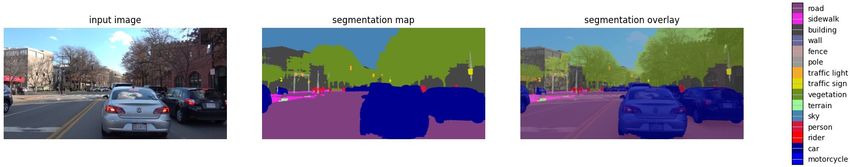
I confirm that this bachelor’s thesis in informatics is my own work and I have documented
all sources and material used.

Potsdam, February 2nd, 2021                              Mahmoud Abdelrahman

Acknowledgments

I would like to thank the following people, without whom I would not have been able to
complete this thesis, and without whom I would not have made it through my bachelor’s
degree!

My supervisor at Volkswagen Car.Software Organisation Mr. Abhishek Saurabh, whose
dedicated support, guidance, encouraging and motivation steered me through this research.

Professor Jochen Heinsohn and Mr. Ingo Boersch at Brandenburg University of Applied
Sciences for agreeing on the supervision.

My family at home for their continuous and unlimited support and encouragement during
my undergraduate years.
Zusammenfassung

In den letzten Jahren hat die Edge-KI, d.h. die Übertragung der Intelligenz von der Cloud in
Edge-Geräten wie Smartphones und eingebetteten Geräten an großer Bedeutung gewonnen
bzw. gewinnt immer mehr an Bedeutung. Dies erfordert jedoch optimierte Modelle für
maschinelles Lernen (ML), die auf Computern mit begrenzten Kanten funktionieren können.
Die Quantisierung ist eine der essenziellsten Techniken zur Optimierung von ML-Modellen.
Es reduziert die Präzision der Zahlen, die zur Darstellung der Parameter eines Modells
verwendet werden.

In dieser Arbeit wurde die Quantisierung untersucht, insbesondere die Quantisierungstech-
niken nach dem Training, die in TensorFlow Lite (TFLite) verfügbar sind. Ein auf MNIST-
Datensatz trainiertes Bildklassifizierungsmodell und ein auf dem Cityscapes-Datensatz trai-
niertes semantisches Segmentierungsmodell wurden für die Durchführung von Experimenten
eingesetzt. Für das Benchmarking wurde die Inferenz auf zwei Hardware-unterschiedlichen
CPU-Architekturen ausgeführt, und zwar auf einem Laptop und einem Raspberry Pi.

Für das Benchmarking wurden Metriken wie Modellgröße, Genauigkeit, mittlere Schnitt-
menge über Vereinigung (mIOU) und Inferenzgeschwindigkeit gehandhabt. Sowohl für
Bildklassifizierungs- als auch für semantische Segmentierungsmodelle zeigten die Ergebnisse
eine erwartete Verringerung der Modellgröße, wenn verschiedene Quantisierungstechniken
angewendet wurden. Genauigkeit und mIOU haben sich in beiden Fällen nicht wesentlich von
der des Originalmodells geändert. In einigen Fällen führte die Anwendung der Quantisierung
sogar zu einer Verbesserung der Genauigkeit. Dabei hat sich die Inferenzgeschwindigkeit
bezüglich des Bildklassifizierungsmodells adäquat verbessert. In manchen Fällen schien aber
bezüglich des semantischen Segmentierungsmodelles doch nicht so der Fall zu sein. In einigen
Fällen erhöhte sich die Inferenzgeschwindigkeit auf Raspberry Pi sogar um den Faktor 10.

                                            iv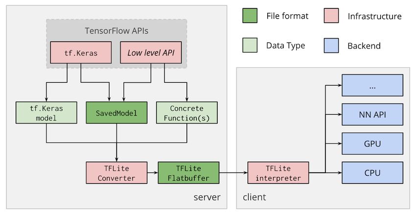
Abstract

In the last few years, edge AI, i.e., moving intelligence from the cloud to the edge devices
like smartphones and embedded devices is gaining traction. But doing so requires optimized
machine learning (ML) models that can work on compute limited edge devices. Quantization
is one of the techniques to optimize ML models. It works by reducing the precision of the
numbers used to represent a model’s parameters.

In this thesis, I have studied quantization, particularly the post-training quantization tech-
niques available in TensorFlow Lite (TFLite). An image classification model trained on MNIST
dataset and a semantic segmentation model, trained on the Cityscapes dataset were used
for performing experiments. For benchmarking, inference was run on two hardware with
different CPU architecture, i.e., a laptop and a Raspberry Pi. Metrics like model size, accuracy,
mean intersection over union (mIOU), inference speed have been used for benchmarking.

For both image classification and semantic segmentation models, results showed an expected
reduction in model size when different quantization techniques were applied. Accuracy
and mIOU, in both the cases didn’t change by a huge margin from that obtained on the
original model. In fact, in some cases, applying quantization actually led to an improvement
in accuracy. The inference speed regarding the image classification model has improved
adequately. On the other hand, no improvement was obtained on inference speed concerning
the semantic segmentation model. In fact, in some cases, latency on Raspberry Pi increased
by a factor of 10.

                                               v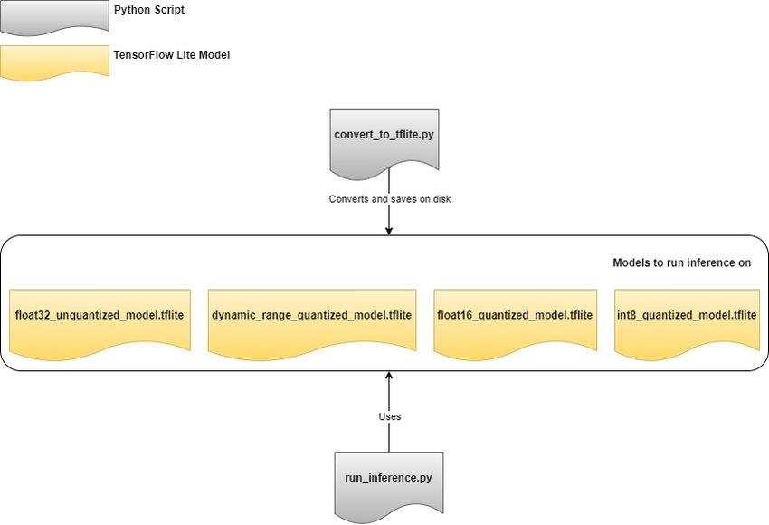
Contents

Acknowledgments                                                                                                                                    iii

Zusammenfassung                                                                                                                                    iv

Abstract                                                                                                                                            v

1   Introduction                                                                                                                                    1
    1.1 Goal of the thesis . . . . . . . . . . . . .   .   .   .   .   .   .   .   .   .   .   .   .   .   .   .   .   .   .   .   .   .   .   .    2
    1.2 A brief Overview of Neural Networks .          .   .   .   .   .   .   .   .   .   .   .   .   .   .   .   .   .   .   .   .   .   .   .    2
         1.2.1 Structure . . . . . . . . . . . . . .   .   .   .   .   .   .   .   .   .   .   .   .   .   .   .   .   .   .   .   .   .   .   .    3
         1.2.2 Training . . . . . . . . . . . . . .    .   .   .   .   .   .   .   .   .   .   .   .   .   .   .   .   .   .   .   .   .   .   .    4
         1.2.3 Inference . . . . . . . . . . . . . .   .   .   .   .   .   .   .   .   .   .   .   .   .   .   .   .   .   .   .   .   .   .   .    5
    1.3 Convolutional Neural Network (CNN)             .   .   .   .   .   .   .   .   .   .   .   .   .   .   .   .   .   .   .   .   .   .   .    5

2   Literature Survey                                                                                                                               7
    2.1 Quantization Fundamentals . . . . . . . . . . . . . .                      .   .   .   .   .   .   .   .   .   .   .   .   .   .   .   .    7
         2.1.1 A brief overview of quantization . . . . . . .                      .   .   .   .   .   .   .   .   .   .   .   .   .   .   .   .    7
         2.1.2 Benefits of quantization . . . . . . . . . . . .                    .   .   .   .   .   .   .   .   .   .   .   .   .   .   .   .    7
         2.1.3 The math behind Full Integer Quantization .                         .   .   .   .   .   .   .   .   .   .   .   .   .   .   .   .    8
         2.1.4 The Anatomy of a quantized layer . . . . . .                        .   .   .   .   .   .   .   .   .   .   .   .   .   .   .   .   10
         2.1.5 Fake quantization nodes . . . . . . . . . . . .                     .   .   .   .   .   .   .   .   .   .   .   .   .   .   .   .   12
    2.2 Related Works . . . . . . . . . . . . . . . . . . . . . .                  .   .   .   .   .   .   .   .   .   .   .   .   .   .   .   .   12

3   Approach                                                                                                                                       16
    3.1 Image classification using MNIST dataset . . . . . . . . . . .                                 .   .   .   .   .   .   .   .   .   .   .   16
    3.2 Semantic segmentation using Cityscapes dataset . . . . . . .                                   .   .   .   .   .   .   .   .   .   .   .   21
    3.3 Quantization . . . . . . . . . . . . . . . . . . . . . . . . . . . .                           .   .   .   .   .   .   .   .   .   .   .   22
        3.3.1 Post-training dynamic range quantization technique                                       .   .   .   .   .   .   .   .   .   .   .   23
        3.3.2 Post-training float-16 quantization technique . . . . .                                  .   .   .   .   .   .   .   .   .   .   .   24
        3.3.3 Post-training full integer quantization technique . . .                                  .   .   .   .   .   .   .   .   .   .   .   24
    3.4 Loading the TensorFlow-Lite model for inference run . . . .                                    .   .   .   .   .   .   .   .   .   .   .   25

4   Experiment design                                                                                                                              26
    4.1 Hardware . . . . . . . . . . . . . . . . . . . . . . . . . . . . . . . . . . . . . . . .                                                   26
    4.2 Software . . . . . . . . . . . . . . . . . . . . . . . . . . . . . . . . . . . . . . . . .                                                 26
        4.2.1 TensorFlow . . . . . . . . . . . . . . . . . . . . . . . . . . . . . . . . . . .                                                     26

                                                  vi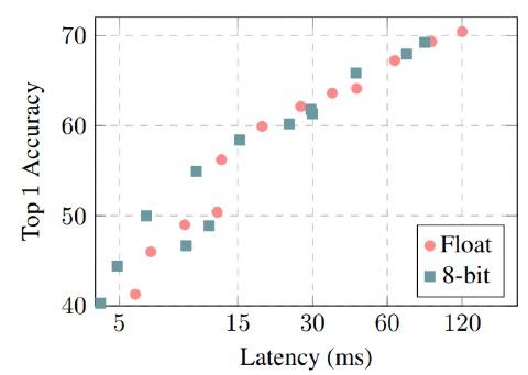
Contents

          4.2.2 TensorFlow Lite (TFLite) .      .   .   .   .   .   .   .   .   .   .   .   .   .   .   .   .   .   .   .   .   .   .   .   .   .   .   .   27
          4.2.3 Docker . . . . . . . . . . .    .   .   .   .   .   .   .   .   .   .   .   .   .   .   .   .   .   .   .   .   .   .   .   .   .   .   .   27
    4.3   System design . . . . . . . . . . .   .   .   .   .   .   .   .   .   .   .   .   .   .   .   .   .   .   .   .   .   .   .   .   .   .   .   .   28
    4.4   Metrics for benchmarking . . . .      .   .   .   .   .   .   .   .   .   .   .   .   .   .   .   .   .   .   .   .   .   .   .   .   .   .   .   29

5   Results and discussion                                                                                                                                  30
    5.1 Results from quantization on MNIST dataset . .                              .   .   .   .   .   .   .   .   .   .   .   .   .   .   .   .   .   .   30
        5.1.1 Change in model size . . . . . . . . . . .                            .   .   .   .   .   .   .   .   .   .   .   .   .   .   .   .   .   .   30
        5.1.2 Accuracy . . . . . . . . . . . . . . . . . . .                        .   .   .   .   .   .   .   .   .   .   .   .   .   .   .   .   .   .   31
        5.1.3 Inference run time . . . . . . . . . . . . .                          .   .   .   .   .   .   .   .   .   .   .   .   .   .   .   .   .   .   31
        5.1.4 Model size vs accuracy tradeoff . . . . .                             .   .   .   .   .   .   .   .   .   .   .   .   .   .   .   .   .   .   32
        5.1.5 inference run time vs accuracy tradeoff .                             .   .   .   .   .   .   .   .   .   .   .   .   .   .   .   .   .   .   33
    5.2 Cityscapes-dataset model quantization results .                             .   .   .   .   .   .   .   .   .   .   .   .   .   .   .   .   .   .   35
        5.2.1 Change in model size . . . . . . . . . . .                            .   .   .   .   .   .   .   .   .   .   .   .   .   .   .   .   .   .   35
        5.2.2 Inference run time . . . . . . . . . . . . .                          .   .   .   .   .   .   .   .   .   .   .   .   .   .   .   .   .   .   35
        5.2.3 Frames per second . . . . . . . . . . . . .                           .   .   .   .   .   .   .   .   .   .   .   .   .   .   .   .   .   .   36
        5.2.4 Pixel accuracy . . . . . . . . . . . . . . . .                        .   .   .   .   .   .   .   .   .   .   .   .   .   .   .   .   .   .   37
        5.2.5 Mean class IoU . . . . . . . . . . . . . . .                          .   .   .   .   .   .   .   .   .   .   .   .   .   .   .   .   .   .   37
        5.2.6 Model size vs frames per second tradeoff                              .   .   .   .   .   .   .   .   .   .   .   .   .   .   .   .   .   .   40
        5.2.7 Model size vs pixel accuracy tradeoff . .                             .   .   .   .   .   .   .   .   .   .   .   .   .   .   .   .   .   .   40
        5.2.8 Model size vs mean class IoU tradeoff . .                             .   .   .   .   .   .   .   .   .   .   .   .   .   .   .   .   .   .   41

6   Conclusion                                                                                                                                              42
    6.1 Outlook . . . . . . . . . . . . . . . . . . . . . . . . . . . . . . . . . . . . . . . . . .                                                         43

List of Figures                                                                                                                                             44

List of Tables                                                                                                                                              46

Bibliography                                                                                                                                                47

                                                    vii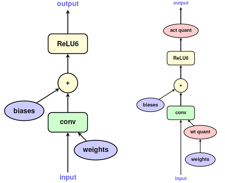
1 Introduction

In the last few years, deep neural networks (DNNs) have achieved remarkable image
classification performance, natural language processing, speech translation, etc. To a large
extent, this performance gain can be attributed to an increase in network size. These
huge networks are usually trained on workstations with powerful GPUs resulting in large
models. Even performing inference on these models is computationally demanding. As such,
they’re often deployed in large data centers as a cloud back-end for edge devices such as
smartphones that cannot process input data in a reasonable time.

However, there’s an increasing push to transition inference execution on edge. The
reasons for this push can be quite varied. Following are a few concerns driving the need for
local processing.

   • Reliability: Relying on an internet connection isn’t often a viable option.

   • Low latency: Delay in sending the inference data to the cloud might now be tolerable
     in latency-critical applications like highly automated driving.

   • Privacy: If inference involves users’ personal data, there could be a legal requirement
     on data not leaving the device.

   • Bandwidth: Network bandwidth is often a key concern. Connecting to the server for
     every use case is not feasible.

   • Power consumption: Transferring data consumes power. Minimizing power consump-
     tion is a priority for embedded systems.

Enabling inference on the edge devices requires overcoming many unique technical challenges
stemming from the distinction of hardware and software [1], one usually doesn’t come across
in a controlled data center environment. As such, regardless of the performance gain, a DNN
might promise, one cannot use it on edge. As an example, while in theory, the performance
of driving assistance functions like Automatic Emergency Braking (AEB) can be improved by
using a state-of-the-art model for semantic segmentation, it is nearly impossible to perform
inference on existing electronic compute units (ECUs) which are significantly compute limited.
This necessitates the need for optimizing DNN models so that state-of-the-art models can be
brought to the edge.

                                              1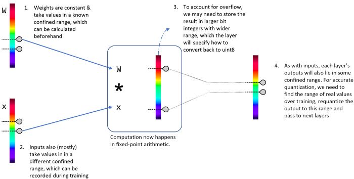
1 Introduction

1.1 Goal of the thesis

The primary objective of this thesis would be two-fold. One, to understand how quantization
works for optimizing deep learning models. This will essentially involve understanding
various types of quantizations and their implementation in TensorFlow Lite (TFLite) [2].

After having developed an understanding on quantization, the second objective would be
to benchmark two or more quantization techniques in TFLite for image classification and
semantic segmentation which are critical to developing the perception system for advanced
driving assistance systems and highly automated driving.

Examples of performance metrics which shall be used for benchmarking are: accu-
racy, model size, inference speed (number of inferences per second), memory usage et cetera.

Auxiliary objective of the thesis will be to familiarize myself with ARMx64 CPU ar-
chitecture, typically used in mobile devices. A natural corollary of this would be to
understand how program compilation works for alternate CPU architectures.

1.2 A brief Overview of Neural Networks

This section gives a brief overview of deep neural networks, including the structure, the
training-, inference-processes, and a brief explanation of different layers.
Before discussing the concept of neural networks, a brief introduction to artificial intelligence,
machine learning, and deep learning is noted.

Artificial Intelligence is the attempt to automate logical tasks typically carried out
by human beings. Consequently, AI is a vast field that encircles machine learning and deep
learning, in addition to many more approaches that do not relate to any learning (François
Chollet 2017 [3], P. 2).

Machine Learning is different from classical programming; in Machine Learning,
humans input data, the answers expected from the data, and output would be the rules.
However, in classical programming, rules and data will be given as input. The data is to be
processed according to these rules, and out would come answers (François Chollet 2017 [3], P.
3).

Deep learning is a subfield of machine learning. Deep Learning corresponds to the
concept of using consecutive layers of representations to model the data. The number of
layers defines the "depth" of the model (François Chollet 2017 [3], P. 6). "In deep learning,
these layered representations are learned via models called "neural networks", structured in

                                                2
1 Introduction
literal layers stacked one after the other" (François Chollet 2017 [3], P. 6).
1.2.1 Structure
The basic form of a deep neural network is composed of artificial neurons that are combined
in layers. The most common DNN architecture consists of an input layer, one or more hidden
layers, and an output layer. Artificial Neurons have some inputs, which come directly from
the data or the output of other neurons. The output of an artificial neuron is only one. This
means that the mechanism inside the neuron combines all inputs and produces a single
output value. So one purpose of the neural network is to propagate values from one neuron
to the next.
Figure 1.1: Simplified view of a feedforward artificial neural network.
Source: Wikipedia, URL: Here, January 06, 2021
Artificial Neuron Architecture
For each of the inputs, there is a unique trainable weight. This allows the neurons to adjust
the importance of each input. The inputs and weights are combined by multiplying each
input (I) times it’s weight (W) and sum them. For a better prediction, there would be a need
to shift the results of summing to adjust the output. So a trainable bias is added. In order to
get access to a much richer hypothesis space that would benefit from deep representations,
we need a non-linearity, or activation function (François Chollet 2017 [3], P. 65). The most
31 Introduction
popular activation function is the ReLU (Rectified Linear Unit) function. ReLU is a function
meant to zero-out negative values (François Chollet 2017 [3], P. 63).
Figure 1.2: A modified simple model of an artificial neuron.
Source: Wikimedia, URL: Here, January 05, 2021
1.2.2 Training
Training a neural network means that the network is learning by predicting the test data. The
predicted result is compared to the provided label. Whenever there is a match, the weights
are increased or decreased if there was no match.
One important specification before inputting the data to a neural network is the in-
put shape, which specifies the batch size, height, width of the picture, and the number of
channels. The height and width of a picture specify the number of pixels in the corresponding
direction. The number of channels is dependent on the type of the input picture; when it is
colored (RGB picture), the number of channels has to be 3. In the case of a black/white or
gray-scale picture, the number of channels is 1.
Batches are the generated sets or parts after dividing the whole dataset, as the dataset cannot
be passed at once. Batch size is the number of training samples piped through the network
in a single batch. An epoch indicates passing an entire dataset through the neural network
for one time only. An iteration is the number of batches needed to complete one epoch. A
dataset of 10,000 examples could be split into batches of 1000; then it takes 10 iterations to
complete one epoch [4].
After the neural network training is finished, it could be saved as a model, which
can be later loaded for additional training or inference run.
41 Introduction
1.2.3 Inference
Inference means using a trained neural network model to predict new data. Similar to
the training process, an input is presented to the network to be processed. The difference
between the inference and training processes is that the output is not compared to a label
for verification in inference. Instead, the class that has the highest probability is taken as a
prediction for the input.
1.3 Convolutional Neural Network (CNN)
A convolutional neural network (CNN) is a class of DNNs in deep learning commonly
applied to computer vision. The hidden layers in a CNN structurally involve convolutional
layers, activation function, pooling layers, fully connected layers (dense layers), and
normalization layers. CNN pulls an input image, processes it, and classifies it under certain
categories (Eg., Car, Person, Horse) by assigning importance (learnable weights and biases) to
different aspects/objects in the image and be capable of differentiating one from the other.
Since 2012, deep convolutional neural networks ("convnets") have been the main algorithm
for all computer vision tasks (François Chollet 2017 [3], P. 16).
The main role of the ConvNet is reducing the image into a form that could be eas-
ily processed without losing critical features to get a good prediction.
Convolutional Layer
The convolutional layer is responsible for capturing low-level features such as edges, color,
etc. This features capturing is done by applying a smaller matrix, called a filter, over the
matrix representing the picture. The filter has predefined values that describe the shape of
the feature to be extracted. For each filter’s position, the dot product is performed. This
process is illustrated in figure 1.3.
Stride determines the number of pixels by which the filter matrix is slid over the in-
put matrix. When the stride is 1, then the filter is shifted one pixel at a time. If the stride is 2,
then the filters shift 2 pixels at a time.
Zero-padding: Sometimes, it is advantageous to pad the input matrix with zeros
around the border so that the filter can be applied to the bordering elements of the input
image matrix.
51 Introduction
Figure 1.3: Outline of the convolutional layer.
Source: Yakura et al. URL: Here, January 8, 2021.
Pooling Layer
Pooling layers are commonly inserted after convolutional layers when constructing CNNs. The
purpose of inserting this layer is to reduce the representation’s spatial size, which successively
reduces the parameter counts, which results in computational complexity reduction. A
pooling size between the maximum, average, or sum values inside these pixels is selected to
reduce the parameters.
A 2*2 filter is generally used for pooling as the main aim is to reduce the pixels and not
extract features. Max Pooling is commonly used, and it works by taking the maximum value
from the 2*2 pixels and eliminates the remaining pixels. Figure 1.4 illustrates an example of a
Max Pooling operation.
Figure 1.4: Max-Pooling by 2*2.
Source: Wikipedia, URL: Here, January 8, 2021
A Flatten Layer aims to transform an input matrix to a single-dimensional set (vector).
A Dense Layer are the simplest layers as they connect every single neuron of one layer with
every single neuron of another layer.
62 Literature Survey
2.1 Quantization Fundamentals
2.1.1 A brief overview of quantization
Quantization in Deep Learning refers to converting a neural networks’ weights and activations
from floating-point format to a fixed point integer format. It works by lessening the number
of bits needed to represent the information contained in a DNN model. DNNs involve
the computations of weight parameters and activation functions. It is these computations
that can be optimized. For perspective, it must be noted that the number of computations
(multiplications and additions) involved in a DNN can very well be of the order of millions.
Mathematical operations with quantized parameters, including intermediate calculations, can
result in large computational gains and higher performance [5].
2.1.2 Benefits of quantization
It is faster to perform mathematical operations with lower bit-depth if the hardware supports
it [6]. Moreover, floating-point arithmetic is complicated [6]. For that reason, it is not
supported on low-power embedded devices. Oppositely, integer support is broadly available
[6]. Operations with 32-bit floating-point are consistently slower than 8-bit integers [6]. By
using 32-bit instead of 8-bits, the memory being used is reduced by a factor of 4 [6]. That
achieves less storage space, easier sharing over smaller bandwidths, and easier updates [6].
These lower bit-widths mean squeezing more data into the same caches/registers, which
reduces the number of times there is a need to access things from RAM, which mostly
consumes a lot of time and power [6].
Why quantization is a good idea for Deep Neural Networks?
DNNs are well-known for being robust to disturbances once trained, which means even if
there is a round off happening to the numbers, there is a big chance to get a reasonably
accurate answer. If the quantization is done right, it will cause a small loss of precision,
72 Literature Survey
which does not significantly impact the output. Small accuracy-losses can also be recovered
by retraining the models to adjust to quantization ([6], [7]). In the histogram below (see
figure 2.1), an example of the weights in a layer from AlexNet [6]. On the histogram’s left side,
the actual weights are shown, concentrated in a small range. On the right side, the weights
are shown after quantizing the range to only record several values from them accurately and
by rounding off the rest (using only 4-bits). An improvement is yet to be achieved with a less
stringent bit-length of 8.
Figure 2.1: A histogram is showing the difference between the ranges representing the actual
weights (on the left) and the 4-bit quantized weights (on the right) in an AlexNet
convolutional neural network architecture.
Source: Manas Sahni, URL: Here, January 15, 2021
2.1.3 The math behind Full Integer Quantization
Low precision
Computers normally use a restricted number of bits to represent unlimited/infinite real
numbers [6]. While the 32-bit floating-point is the default binary number format used in most
applications, including deep learning [6]. It turned out that DNNs can work with a smaller
datatype with less precision, such as an 8-bit integer [6]. The numbers are discretized to
specific values, which can be represented using integers instead of floating-point numbers [6].
Floating-point binary format
Floating-point formats are frequently used to represent real values [8]. They include a sign,
an exponent, and a mantissa [8]. Because of the exponent, the floating-point format is given a
wide range, and the mantissa gives it a good precision [8].
82 Literature Survey
Fixed-point binary format
In the fixed-point format, the exponent is replaced by a fixed scaling format, which is shared
among all the fixed-point numbers [8].
Figure 2.2: Comparison of the floating point and fixed point formats.
Source: Courbariaux et al. [8], January 15, 2021
Full Integer Quantization scheme
To accurately map real numbers to quantized numbers, two main requirements for the
scheme must be achieved: 1- It should be linear (affine), so that it is possible to map the
fixed-point calculation back to a real number. 2- Because of the important role that the zero
plays in the DNNs (padding, for example) and also that the zero maps to another value that
is higher/lower than it, the quantization scheme must always represent the 0.f accurately ([7],
[6]).
For a given set of real numbers, the minimum/maximum real values in this range
[rmin, rmax] are mapped to the minimum/maximum integer values [0, 2B − 1], where B is
the number of bits used ([7], [6]). That translated into an equation ([7], [6]):
rmax − rmin
r= × (q − z)
(2 B − 1) − 0 (2.1)
= S × (q − z)
• r refers to the real value (usually float32)
• q refers to the quantized representation as a B-bit integer.
92 Literature Survey
• S(float32) and z(uint) refer to the factors by which the scaling and shifting done on the
number line. z is the quantized ’zero-point’ which maps always to 0.f.
Figure 2.3: Illustration of the mapping process between the real numbers and quantized
numbers using a line number (orange to blue respectively).
Source: Manas Sahni, URL: Here, January 15, 2021
2.1.4 The Anatomy of a quantized layer
Before discussing the specifications of a quantized layer, a brief overview of a conventional
layer in floating-point is to be given.
The Specifications of a layer in Float
• Zero to N constant weight tensors are stored in float [6].
• One to N input tensors are also stored in float [6].
• The forward pass process that works on the weights and inputs is using floating-point
arithmetic. After the forward pass function is done with its work, the output will be
stored in float [6].
• The output Tensors’ format is float.
A quantized layer’s anatomy
Keeping in mind that the weights of a pre-trained network are constant [6]. They can be
converted and stored in the quantized form beforehand with their exact ranges known [6].
The input to the layer and equivalently the output of the previous one are usually quantized
102 Literature Survey
with their own parameters [6]. While it is ideal to know the exact range of values to quantize
them [6] with the best accuracy possible, results of unknown inputs can, to a good extent, be
in similar bounds. As the output is already computed in float during training, the average
output range on many inputs can be used as a proxy to the output quantization parameters
[6]. When an actual unseen input is being processed, an outliner will be squashed if the
range is small, or it will be rounded if the range is wide, with the hope that will be only a
few of these unseen inputs ([7], [6]).
Left to be quantized is the main function that computes the layer’s output. Chang-
ing this to a quantized version is more complex [6]. A simple changing from float to int
everywhere would not be sufficient, as the integer computations’ results can overflow [6]. A
good method to avoid that is storing the results in larger integers first (int32, for example)
and then requantizing it to the 8-bit output [6]. This might not be a concern when it comes to
a conventional full-precision implementation, where all variables are float, and the hardware
handles all the tiny details of that floating-point arithmetic [6]. Furthermore, some of the
layers’ logic should be changed. A good example is the ReLU, which should now compare
values against Quantized(0) instead of 0.f [6].
Figure 2.4: Illustration of putting together the steps done during the quantization process of
a single neuron.
Source: Manas Sahni, URL: Here, January 15, 2021
112 Literature Survey
2.1.5 Fake quantization nodes
The simplest technique to quantize a neural network is to first train it in full precision and
quantize the weights to fixed-point (Post-Training Quantization) ([7], [6]). This technique
works well for large models, but in the case of a small model with less redundancy regarding
the weights, the precision loss will have a huge impact on the accuracy ([7], [6]). The concept
of TensorFlow’s fake quantization nodes is simulating the rounding effect of quantization
in the forward pass as it would occur while performing actual inference ([7], [6]). In other
words, the weights will be fine-tuned for adjustment for the precision loss ([7], [6]).
Fake quantization nodes could record the ranges of activations during training by
placing them in the training graph in the places where activations would change quantization
ranges (Quantization Aware Training). As the training of the network is running, they gather
a moving average of the ranges of the float values seen at that node ([7], [6]).
The graphs in figure 2.5 represent how the TensorFlow framework uses the fake quantization
nodes. In the case of integer-arithmetic-only inference of a convolution layer (shown in
the left graph), the input and output will be represented as 8-bit integers according to the
quantization scheme 2.1 ([7], [6]). The convolution necessitates 8-bit integer operands and
a 32-bit integer accumulator. The bias addition involves only 32-bit integers. The ReLU
nonlinearity only involves 8-bit integer arithmetic ([7], [6]).
On the right graph, training with simulated quantization of the convolution layer is illustrated
([7], [6]). All variables and computations are performed with arithmetic in 32-bit floating-
point. (wt quant) which stands for weight quantization and activation quantization (act
quant) nodes are fitted into the graph to fake the effects of quantization of the variables.
The resultant graph approximates the integer-arithmetic-only computation graph (in the left
graph) while being trainable using conventional optimization algorithms for floating-point
models ([7], [6]).
2.2 Related Works
Jacob et al. proposed in [7] a scheme that allows carrying out inference in integer-only
arithmetic, which can be implemented more efficient than the floating-point variant on the
available integer-only hardware. This quantization scheme quantizes both weights and
activations as 8-bit integers and just a few parameters (bias vectors) as 32-bit integers [7].
This framework is implementable on integer-arithmetic-only hardware. A quantized training
framework was also designed with the quantized inference framework to minimize the
accuracy loss. Those developed frameworks were applied on efficient classification and
detection systems based on MobileNets convolutional neural networks.
122 Literature Survey
Figure 2.5: Integer-arithmetic-only quantization with fake quantization nodes graphs.
Source: Jacob et al. [7], January 15, 2021
The benchmark results on popular ARM CPUs were provided in this paper. There
were significant improvements in the latency-vs-accuracy tradeoffs for the state-of-the-art
MobileNet architectures, demonstrated in the ImageNet classification and COCO object detec-
tion [7]. Three micro-architectures were used for the experiments: 1) Snapdragon 835 LITTLE
core which is found in Google Pixel 2. 2) Snapdragon 835 big core, a high-performance core
employed by Google Pixel 2. 3) Snapdragon 821 big core, a high-performance core used in
Google Pixel 1 [7].
Integer-only quantized MobileNets achieved higher accuracies than floating-point
with the same runtime (see figure 2.6) [7]. Important thing to note is the critical tradeoff
dependency on the relative speed of floating-point vs integer-only arithmetic in hardware.
Floating-point computation is finer optimized in the Snapdragon 821, for example, resulting
in a less detectable reduction in latency for quantized models (see figure 2.7).
132 Literature Survey
Figure 2.6: ImageNet latency-vs-accuracy tradeoff on Snapdragon 835 LITTLE core.
Source: Jacob et al. [7], January 15, 2021
Figure 2.7: ImageNet latency-vs-accuracy tradeoff on Snapdragon 821 big core.
Source: Jacob et al. [7], January 15, 2021
142 Literature Survey
Courbariaux et al. [8] trained a set of state-of-the-art neural networks with three distinct
formats: floating point, fixed point and dynamic fixed point on three different dataset:
MNIST [9], CIFAR-10 and SVHN [8]. The effect of the precision of the multiplications on the
final error after training was assessed [8]. Found out was that very low precision is sufficient
not just for running trained networks but also for training them [8].
Wu et al.[1] outlined the two-fold problem: Although there is a strong need to bring
AI to edge devices, there is a heap of dissimilar parts, dissimilar software APIs, and overall
poor performance. Another important complication is the nonexistence of a standard mobile
SoC (System on a Chip) to optimize for.
The authors have also identified that machine learning performance slightly differs
across different "tiers" of hardware. Some low-tier phone models perform better than the
mid-tier models, translating directly into a varied user experience quality.
153 Approach
During the thesis, the approach was converting the TensorFlow model into TensorFlow-
Lite models, applying the three quantization techniques provided by TensorFlow-Lite, run
inference on the unquantized model, and quantized models. Finally, report the results.
The models used during the thesis are for the image classification and semantic image
segmentation tasks.
This chapter provides an overview of the image classification and semantic image segmenta-
tion tasks, their common evaluation metrics, and the datasets used to train the models used
for those tasks. Moreover, it explains how TensorFlow Lite is being used to convert original
models into TensorFlow Lite models and load them for inference run.
While the thesis was meant to run inference on pre-trained models, the MNIST dataset
training was performed before the inference run. Reasons for that are:
• Getting an idea, how training works and understanding the architecture of a convolu-
tional neural network and the layers it contains practically by defining the architecture
in Python programming language.
• The MNIST dataset is not large, it can be loaded with the Keras interface, and it takes
only minutes to train it.
On the other hand, a model that has been trained on the Cityscapes dataset has been used to
run inference in the semantic image segmentation task.
3.1 Image classification using MNIST dataset
Image classification is the task of analyzing an image and identifying the ’class’ the image
falls under. A class is necessarily a label, for instance, ’car’, ’animal’ and so on [10]. Image
classification is considered one of the fundamental computer vision problems, and it also
forms the basis for other computer vision problems.
In image classification, accuracy is the most common evaluation metric. Accuracy is how
many times the model has predicted the right label of an image, divided by the number of
test samples.
163 Approach
The MNIST dataset [9] from the National Institute of Standards and Technology (NIST)
contains a training set of 60,000 examples and a testing set of 10,000 examples represented in
images of hand-written numbers from 250 different people. Each pattern in the set is of size
28x28 pixels. The dataset can be downloaded from the MNIST dataset official website.
Figure 3.1: Sample of the MNIST dataset.
Source: MNIST dataset on GitHub
For the model training, MNIST dataset is first loaded from the available datasets using the
tf.keras.datasets module. The training and testing sets with their corresponding labels are
saved in a tuple contains Numpy arrays. After the dataset is loaded, a normalization step has
to take place.
Normalization is a technique used to prepare the data for machine learning. This
technique aims to change the value of numeric columns in the dataset to a common scale [11].
This technique is required when features have different ranges.
To make learning easier for the network, the data should take small values. Typi-
cally, most values should be in the 0-1 range. As in code listing 3.1, the input train- and
test-images will be normalized by dividing each pixel value of the images by 255.0.
1 train_images = train_images.astype(np.float32) / 255.0 # np is NumPy
2 test_images = test_images.astype(np.float32) / 255.0 # np is NumPy
Code Listing 3.1: Code example for the normalization of the images’ pixel values [12]
The model is structured sequential, which means that it is built one layer at a time to solve a
problem. There is a 28 x 28 shape in the input layer, representing the image’s dimensions
that the model will process. The shape will then be reshaped to a 28 x 28 shape and a third
dimension, representing the number of channels. As the dataset contains only grayscale
images, the number of channels is only one.
173 Approach
By making use of a convolution, certain features in the image get emphasized. 12
filters of 3 x 3 dimensions have been used. Relu activation function is used to zero-out
negative values, which means if the number generated is bigger than 0, this number will be
passed to the next layer. Otherwise, 0 will be passed.
There is then a pooling layer added to the architecture. Pooling will be applied by
using a 2 x 2 pixels filter. Max-pooling has been used, which means that the biggest pixel will
survive out of every four pixels.
That generated images from the pooling layers will be then flattened into a single-
dimensional set.
In the end, a layer of neurons is added using the Dense function. This layer uses
softmax function to return an array of 10 probability scores (summing to 1). Each score will
be the probability that the current digit image belongs to one of the 10 digit classes (François
Chollet 2017 [3], P. 24).
Those steps are implemented in the code listing 3.2. A visual representation of the neural
network after executing this code is shown in figure 3.2.
1 model = tf.keras.Sequential([
2 tf.keras.layers.InputLayer(input_shape = (28,28)),
3 tf.keras.layers.Reshape(target_shape = (28,28,1)),
4 tf.keras.layers.Conv2D(filters=12, kernel_size = (3, 3), activation = "relu"),
5 tf.keras.layers.MaxPooling2D(pool_size = (2,2)),
6 tf.keras.layers.Flatten(),
7 tf.keras.layers.Dense(10)
8 ])
Code Listing 3.2: Code example for defining the architecture of the image classification model
[12].
183 Approach
Figure 3.2: Visual presentation of the MNIST image classification model.
193 Approach
Before the network is ready for training, three things come into use in the compilation process
(see code listing 3.3):
• A loss function: It is how the network measures the quality of the training. Depending
on that measurement, the network will steer itself in the right direction. In this case, the
Space Categorical Crossentropy function is used, which is typically used when there
are two or more label classes.
• An optimizer: It is the mechanism, which the network uses to update itself based on
the data and loss function (François Chollet 2017 [3], P. 24). Here is the Adam optimizer
used. Adam is an optimization algorithm that can be used to update network weights
iterative based on training data [13].
• The "accuracy" value in the metrics parameter is used to calculate how often predictions
equal labels.
1 model.compile(optimizer="adam",
2 loss=tf.keras.losses.SparseCategoricalCrossentropy(
3 from_logits=True),
4 metrics=["accuracy"])
Code Listing 3.3: Code example for compiling a model [12].
The fit method will train the model by repeatedly iterating over the entire dataset for a given
number of "epochs" [14] (see code listing 3.4).
1 model.fit(train_images,
2 train_labels,
3 epochs=5,
4 validation_data=(test_images, test_labels)
5 )
Code Listing 3.4: Code example for training a model
After the training phase is done, the model is then saved as a (.h5: Hierarchical Data Format)
file. The file can be used for further training or to run inference on (see code listing 3.5).
1 model.save("model.h5")
Code Listing 3.5: Code example for saving a trained TensorFlow model [12].
203 Approach
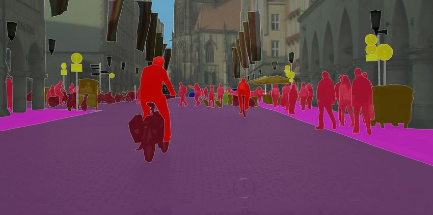
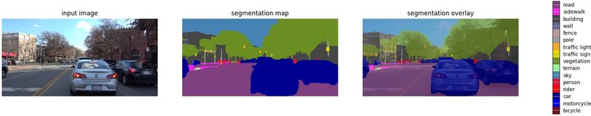
3.2 Semantic segmentation using Cityscapes dataset
Semantic image segmentation, which is also called pixel-level classification, is the task of
labeling each pixel to a corresponding class [15]. Semantic image segmentation has become
one of the key applications in the computer vision domain. It has been used in multiple areas
such as the Advanced Driver Assistance Systems (ADAS), self-driving car and medical image
diagnostics [16]. Evaluation metrics in this task are:
1. Pixel accuracy: It is the percentage of the correctly classified pixels in an image. This
metric is not frequently used, as the high pixel accuracy does not necessarily suggest
high-level segmentation ability.
2. Mean intersection over union (IoU): It is a more-frequent used metric for semantic image
segmentation. It is the overlap between the predicted segmentation and the ground
truth divided by the area of union between the predicted segmentation and the ground
truth [17]. It works by computing the intersection over union for each semantic class
and then computing the average over classes. IoU is calculated using the following
scheme:
TP
IOU = (3.1)
TP + FP + FN
• True Positive (TP): The number of accurately classified pixels belonging to class X.
• False Positive (FP): The number of pixels that do not belong to class X in ground
truth but are classified as that class by the algorithm.
• False Negative (FN): The number of pixels that do belong to class X in the ground
truth but are not classified as that class by the algorithm.
3. Frames per second: The number of frames being processed during the inference in one
second.
For the training and inference, the Cityscapes dataset ([18], [19]) has been used. It contains
a large, diverse set of 25,000 images in streets from 50 different cities. It contains 30 classes
grouped in 8 groups (see table 3.1).
During the thesis, 19 classes (underlined in the table 3.1) have been used in the semantic
image classification task while performing inference.
The pre-trained model was downloaded from the Available TensorFlow DeepLab models.
213 Approach
Group Classes
flat road, sidewalk, parking, rail track
human person, rider
vehicle car, truck, bus, on rails, motorcycle, bicycle, caravan, trailer
construction building, wall, fence, guard rail, bride, tunnel
object pole, pole group, traffic sign, traffic light
nature vegetation, terrain
sky sky
void ground, dynamic, static
Table 3.1: Cityscapes dataset classes.
Source: Cityscapes dataset overview
Figure 3.3: Cityscapes dataset sample.
Source: Cityscapes dataset overview
3.3 Quantization
After the model is trained and saved, it can then be loaded to be used for inference. The
Python API for TensorFlow Lite supports the conversion from several file types [20]. This
thesis focuses on only two file types: Keras model for the classification-MNIST dataset model
and frozen inference graph for the image semantic segmentation-Cityscapes dataset model.
As shown in the code listing 3.6, the TFLite Converter has been used to convert the Keras
model to a TensorFlow Lite model.
In the case of the semantic segmentation-Cityscapes dataset, the model was converted from
the model graph and model weights definition (.pb: protcol buffer) to a TensorFlow Lite
223 Approach
model (see code listing 3.7). The input and output arrays have to be defined while converting
from a frozen inference graph. This information can be called by passing the model to a
neural network viewer, Netron for example.
By invoking the convert() method, the models will be converted. Hence, the models are only
converted to TensorFlow Lite and are not yet optimized.
1 mnist_classification_keras_model = keras.models.load_model("model.h5")
2 converter = tf.lite.TFLiteConverter.from_keras_model(mnist_classification_keras_model)
3 float32_unquantized_model = converter.convert()
Code Listing 3.6: Code example for loading the classification-MNIST model and converting it
to a TensorFlow Lite model
1 converter = tf.compat.v1.lite.TFLiteConverter.from_frozen_graph(
2 graph_def_file="frozen_inference_graph.pb",
3 input_arrays=["sub_7"],
4 output_arrays=["ResizeBilinear_2"]
5 )
6 float32_unquantized_model = converter.convert()
Code Listing 3.7: Code example for loading the semantic segmentation-Cityscapes model and
converting it to a TensorFlow Lite model
3.3.1 Post-training dynamic range quantization technique
Dynamic range quantization is the simplest technique of post-training quantization
techniques. It statically quantizes only the weights from floating-point to 8-bit integer.
During the inference, weights will be converted from 8-bit integers to floating-point and
computed with floating-point kernels. In this technique of quantization, the conversion is
done once and cached to achieve latency reduction. For a further latency improvement,
"dynamic-range" operators dynamically quantize activations dependent on their range to
8-bits. The computations are then performed with 8-bit weights and activations [21].
To quantize a pre-trained model before converting it to TensorFlow Lite, a usage of
the TFLite enum "Optimize" has to be made. The generated model is then a dynamic-range
quantized model with up to a 75% drop in the model size.
This quantization technique is recommended to be used to optimize models for a
later inference run on Central Processing Units (CPUs).
1 converter = tf.lite.TFLiteConverter.from_keras_model(keras_model)
2 converter.optimizations = [tf.lite.Optimize.DEFAULT]
233 Approach
3 dynamic_range_quantized_model = converter.convert()
Code Listing 3.8: Code example for using dynamic-range quantization technique to optimize
a TensorFlow model before converting it to a TFLite model.
3.3.2 Post-training float-16 quantization technique
The second technique of quantization is the float-16 quantization technique. The only
difference from the code used in the dynamic-range quantization is that the target supported
types are limited to float16. The model size is dropped to size up to 50% of the original size
after applying this quantization technique.
This quantization technique is recommended to be used to optimize models for a
later inference run on Central Processing Unit (CPU) and Graphical Processing Unit (GPU).
1 converter = tf.lite.TFLiteConverter.from_keras_model(keras_model)
2 converter.optimizations = [tf.lite.Optimize.DEFAULT]
3 converter.target_spec.supported_types = [tf.float16]
4 float16_quantized_model = converter.convert()
Code Listing 3.9: Code example for using float16 quantization technique to optimize a
TensorFlow model before converting it to a TFLite one
3.3.3 Post-training full integer quantization technique
The third technique used in the experiments during the thesis is the full integer (INT8)
quantization technique. Here in this technique of quantization the target supported types is
limited to 8-bit integer and a representative dataset generator must be used. A representative
dataset is a dataset that can be used to evaluate optimizations by the converter [22]. Same as
the dynamic range quantized model, the model size is down by approximately 75%. An
integer quantized model that uses integer data for the model’s input and output tensors
is generated, so it’s compatible with integer-only hardware such as the Edge TPU (Tensor
Processing Unit) [12].
This quantization technique is recommended to be used to optimize models for a
later inference run on Central Processing Unit (CPU), Edge TPUs, and Microcontrollers.
1 def representative_data_gen():
2 for input_value in tf.data.Dataset.from_tensor_slices(train_images).batch(1).take(100):
3 yield [input_value]
4 converter = tf.lite.TFLiteConverter.from_keras_model(model)
243 Approach
5 converter.optimizations = [tf.lite.Optimize.DEFAULT]
6 converter.representative_dataset = representative_data_gen
7 converter.target_spec.supported_ops = [tf.lite.OpsSet.TFLITE_BUILTINS_INT8]
8 converter.inference_input_type = tf.uint8
9 converter.inference_output_type = tf.uint8
10 int8_quantized_model = converter.convert()
Code Listing 3.10: Code example for using integer-only quantization technique to optimize a
TensorFlow model before converting it to a TFLite model [12].
3.4 Loading the TensorFlow-Lite model for inference run
A use of the TensorFlow-Lite converter is then made to get the input and output details
of the model. As shown in the code listing 3.11, the model path is passed as a parameter
to the Interprter interface to load the model corresponding to the passed path. Through
the interpreter object, the input and output details, that contain the name, shape and
datatype of input and output data of the model are called through get_input_details() and
get_output_details() functions. These information are then assigned to the input_details
and output_details variables respectively.
1 interpreter = tf.lite.Interpreter("float16_quantized_model.tflite")
2 interpreter.allocate_tensors()
3 input_details = interpreter.get_input_details()[0]
4 output_details = interpreter.get_output_details()[0]
Code Listing 3.11: Code example for loading the float-16 quantized model to run the inference
[12].
In most cases there is a mismatch between the input data format expected by the model and
the raw input data. A need to resize an image or change it’s format might exist to achieve the
compatibility with the model.
After the step of resizing or changing the format of the image is done, the input
data is passed through the set_tensor() function. Hereafter, a call to the invoke() function
is made to run the inference on the input data. The argmax() function is then applied to the
output to get the index with the largest value across all tensors (see code listing 3.12).
1 interpreter.set_tensor(input_details["index"], test_image)
2 interpreter.invoke()
3 output = interpreter.get_tensor(output_details["index"])[0]
4 prediction = output.argmax()
Code Listing 3.12: Code example for running inference [12].
254 Experiment design
This chapter briefly explains the hardware and software setup, including a schematic of the
overall system developed for performing the experiments.
4.1 Hardware
For benchmarking purposes, experiments were performed on two a laptop and a Raspberry
Pi. Their specifications are as follows.
• Notebook: HP EliteBook 840 G5 i7-8650U with eight cores and a clock frequency of
1.90 GHz with 16 GB of RAM. It had Ubuntu 20.04 as an operating system.
• Raspberry Pi 4B: It was launched in June 2019 and runs a Debian-based OS optimized
for the Raspberry Pi hardware operating system. The CPU is a Cortex-A72 (ARM v8)
with four cores, and a clock frequency of 1.50 GHz. 4 GB of LPDDR4-3200 RAM are
installed.
4.2 Software
Image classification and semantic segmentation models developed using TensorFlow were
used for performing experiments. For quantizing, TensorFlow Lite (TFLite) was used. These
are briefly described in the following sub-section. The entire setup was developed in a
containerized environment using Docker.
4.2.1 TensorFlow
TensorFlow is an end-to-end open-source platform for machine learning. It has a comprehen-
sive, flexible ecosystem of tools, libraries, and community resources that lets researchers push
the state-of-the-art in ML and developers easily build and deploy ML-powered applications
[23]. TensorFlow was developed and is maintained by Google. It was developed to run
264 Experiment design
on CPUs and GPUs and mobile operating systems, and it has different APIs in several lan-
guages like Python, C++, or Java. Keras is an open-source neural network library developed
by François Chollet and written in Python. It acts as a high-level interface to deal with
TensorFlow.
4.2.2 TensorFlow Lite (TFLite)
TensorFlow Lite is a set of tools to help developers run TensorFlow models on mobile,
embedded, and IoT devices. It enables on-device machine learning inference with low latency
and a small binary size [2]. As shown in figure 4.1, TFLite has two main components.
• Interpreter: Thanks to the little-sized interpreter (approximately 300 KB) that TFLite
comes with, optimized models can be run on different devices with different operating
systems like Android and iOS. TFLite interpreter comes with APIs suited for multiple
languages: on Android, TFLite inference is performed with either Java or C++ applica-
tion programming interfaces; on iOS, there are APIs written in Swift and Objective-C,
and on Linux (including Raspberry Pi), TFLite APIs are available in C++ and Python
[24].
• Converter: converts the TensorFlow or Keras model (.pb or .h5) to a TFLite model (.tflite)
which can be straightaway deployed in those devices. The interpreter can then use the
converted model to perform inference. The converted model is stored in an efficient file
format that uses FlatBuffers, a cross-platform serialization library for most programming
languages, like C++, C, Python, et cetera. FlatBuffers was created at Google for game
development and other performance-critical applications. Optimizations to the model to
reduce the model size, inference time, or both can be done through the TFLite converter
[24].
4.2.3 Docker
Docker is an open-source platform used to provide the ability to put an application in a
package and run it in a separated, isolated environment called a container [25].
Docker has been used to create two docker images to be hosted in the raspberry pi
for the inference run. A separated docker image was created for each of the models
(MNIST-dataset model and CityScapes-dataset model). A Dockerfile was written for every
image, which is a text document that contains all the commands a user could call on the
command line to assemble a docker image [25].
274 Experiment design
Figure 4.1: TensorFlow Lite internal architecture.
Source: TensorFlow Lite Documentation
4.3 System design
Figure 4.2 illustrates the design of the system developed for this thesis. Two python scripts
were written. One of them contains the code required to use the TFLite converter to convert
the pre-trained models into the TFLite unquantized (float32) and quantized models and
then save the resulting model on to the disk. The pre-trained models were in the format
frozen_inference_graph.pb or model.h5. The other script runs inference on those models and
saves the evaluation results and the image output on the disk.
284 Experiment design
Figure 4.2: System design for model conversion and running inference
4.4 Metrics for benchmarking
As noted earlier, experiments were performed on pre-trained models obtained for both image
classification and semantic segmentation. For the former, metrics like model size, inference
run time, and accuracy were studied. The trade-off of these metrics was also analyzed.
For semantic segmentation, metrics like model size, inference run time, mean intersection
over union, pixel accuracy, and inference in frames per second was studied. These metrics are
elaborated in the section Semantic segmentation using Cityscapes dataset.
295 Results and discussion
As noted in the previous chapter, inference was run on a notebook and a Raspberry Pi.
Models trained on MNIST and Cityscapes datasets were used for running inference. Images
in the test set of the respective datasets were used. For the classification problem i.e. the one
with MNIST dataset, following metrics have been reported:
1. Change in model size
2. Accuracy
3. Inference run time
For semantic segmentation i.e. the one with the Cityscapes dataset, following metrics have
been reported:
1. Change in model size
2. Inference run time
3. Frames per second
4. Pixel accuracy
5. Mean class intersection over union (IoU)
5.1 Results from quantization on MNIST dataset
5.1.1 Change in model size
Figure 5.1 shows the change in model size when different post-training quantization tech-
niques are applied. The reduction in model size is as per the expectation, i.e., when fewer
bits represent model parameters, the model size drops.
Dynamic range quantization results in a model that is roughly 25% of the original float32
model. INT8 quantization results in a model that is 29% of the original model. Likewise, the
model obtained after applying float16 quantization is half the size of the original model.
305 Results and discussion
Figure 5.1: Classificaton-MNIST dataset model size before and after quantization (lower is
better).
5.1.2 Accuracy
Figure 5.2 shows the average accuracy obtained after running inference on 10,000 images in
the test set of MNIST. The same accuracy was obtained when inference was run on the laptop
and the Raspberry Pi.
It’s worth noting that while the model size did drop by 2x-4x when quantization was applied,
the accuracy did not suffer much. Even in the worst case, with the INT8 quantized model,
the accuracy is very close to that obtained with the original model. This suggests that the
model is good enough to be deployed on compute-limited devices like an edge TPU or a
microcontroller.
5.1.3 Inference run time
As shown in figure 5.3, quantization type seems to influence inference run time. On the laptop,
the float16 and dynamic range quantized models have less inference run time than the float32
unquantized model by 0.103 seconds and 0.057 seconds, respectively. On Raspberry Pi, the
INT8 quantized model has the least inference run time with 69% less than the original model.
The INT8 quantized models rely on special instructions that have not been emphasized on
Intel x86_64 processors, which leads to better performance on ARM processors. This explains
this result that INT8 quantized model achieves overall better inference runtime on Raspberry
Pi, even better than its counterpart on the laptop. This suggests that the INT8 is once again a
better choice for the deployment on compute-limited edge devices.
31You can also read