Multi-Objective Optimization Method for the Shape of Large-Space Buildings Dominated by Solar Energy Gain in the Early Design Stage
←
→
Page content transcription
If your browser does not render page correctly, please read the page content below
ORIGINAL RESEARCH
                                                                                                                                       published: 03 November 2021
                                                                                                                                     doi: 10.3389/fenrg.2021.744974

                                           Multi-Objective Optimization Method
                                           for the Shape of Large-Space
                                           Buildings Dominated by Solar Energy
                                           Gain in the Early Design Stage
                                           Longwei Zhang *, Chao Wang, Yu Chen and Lingling Zhang
                                           School of Architecture and Urban Planning, Shenyang Jianzhu University, Shenyang, China

                                           Large-space buildings feature a sizable interface for receiving solar radiation, and
                                           optimizing their shape in the early design stage can effectively increase their solar
                                           energy harvest while considering both energy efficiency and space utilization. A large-
                                           space building shape optimization method was developed based on the “modeling-
                                           calculation-optimization” process to transform the “black box” mode in traditional design
                          Edited by:       into a “white box” mode. First, a two-level node control system containing core space
                     Xingxing Zhang,
                                           variables and envelope variables is employed to construct a parametric model of the shape
          Dalarna University, Sweden
                                           of a large-space building. Second, three key indicators, i.e., annual solar radiation, surface
                       Reviewed by:
                            Yilin Song,    coefficient, and space efficiency, are used to representatively quantify the performance in
              Tianjin University, China    terms of sunlight capture, energy efficiency, and space utilization. Finally, a multi-objective
                        Yunsong Han,
Harbin Institute of Technology, China      genetic algorithm is applied to iteratively optimize the building shape, and the Pareto
                     Shuangcheng Yu,       Frontier formed by the optimization results provides the designer with sufficient alternatives
              Northwestern University,
                                           and can be used to assess the performance of different shapes. Further comparative
                         United States
                                           analysis of the optimization results can reveal the typical shape characteristics of the
               *Correspondence:
                                           optimized solutions and potentially determine the key variables affecting building
                    Longwei Zhang
   longweizhang17100@outlook.com           performance. In a case study of six large-space buildings with typical shapes, the solar
                  z_lw@sjzu.edu.cn         radiation of the optimized building shape solutions was 13.58–39.74% higher than that of
                                           reference buildings 1 and 3; compared with reference buildings 2 and 4, the optimized
                  Specialty section:
       This article was submitted to       solutions also achieved an optimal balance of the three key indicators. The results show
    Sustainable Energy Systems and         that the optimization method can effectively improve the comprehensive performance of
                             Policies,
                                           buildings.
              a section of the journal
       Frontiers in Energy Research
                                           Keywords: large-space building, building shape, multi-objective optimization, solar radiation, surface coefficient,
           Received: 21 July 2021          space efficiency
       Accepted: 13 October 2021
     Published: 03 November 2021
                             Citation:     INTRODUCTION
Zhang L, Wang C, Chen Y and Zhang L
  (2021) Multi-Objective Optimization
                                           Due to climate change and a shortage of fossil fuels, clean energy, particularly solar energy, is
Method for the Shape of Large-Space
Buildings Dominated by Solar Energy
                                           increasingly used in buildings. Today, a major direction of sustainable building is designing buildings
       Gain in the Early Design Stage.     to obtain abundant solar energy, which can be converted into electricity or heat (Baljit et al., 2016;
        Front. Energy Res. 9:744974.       Barone et al., 2020; Liu et al., 2021; Maghrabie et al., 2021; Yu et al., 2021). Large-space buildings are
     doi: 10.3389/fenrg.2021.744974        of high research value thanks to their inherent advantages in capturing solar energy.

Frontiers in Energy Research | www.frontiersin.org                               1                                     November 2021 | Volume 9 | Article 744974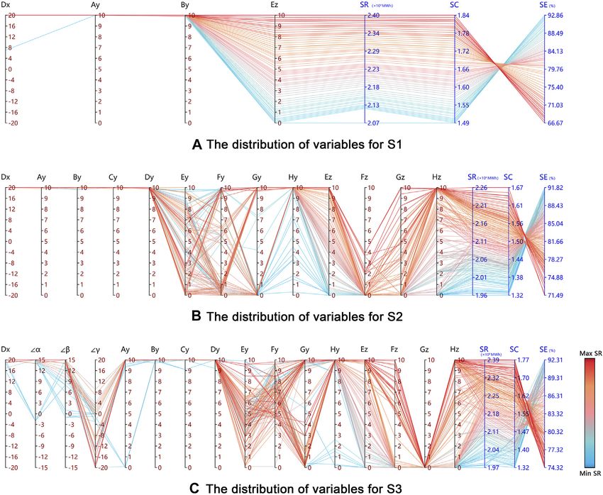
Zhang et al.                                                                                                     Building Design Concerning Solar Energy

 FIGURE 1 | The traditional black box design model.

    Large-space buildings usually refer to buildings with interior             to make progressive improvements (Ascione et al., 2015). This
heights greater than 10 m that are partially used by occupants,                process ensures that concepts with better performance enter the
including exhibition halls, stadiums, theaters, commercial                     subsequent detailed design stage (Negendahl and Nielsen, 2015).
buildings, terminals, and railway stations (Heiselberg et al.,                 The process described above is a “black box” in terms of
1998; Rohdin and Moshfegh, 2007; Li et al., 2009; Gil-Lopez                    traditional design models: the information is input into the
et al., 2017; Liu et al., 2018; Liu et al., 2020). Large-space buildings       mind of the designer to generate and select building concepts,
generally entail high costs and immense energy consumption, but                and the design result is output directly (Harding et al., 2012), as
they have great potential for capturing solar energy. First, the               shown in Figure 1. This process is highly dependent on the
enormous roof areas of these buildings are natural interfaces for              intuition and experience of the designer, neglects quantitative
receiving solar radiation and can collect a large amount of solar              analyses of various measures of the building performance, and
energy. Second, large-space buildings usually have smooth shapes               involves only a small number of concept iterations, making it
that do not change abruptly; therefore, solar irradiation is evenly            difficult to ensure the feasibility and validity of the output result.
distributed on the building surface, which reduces the potential               In this work, we attempt to improve this process by (1) studying
for self-shading (Zhang et al., 2012). Third, large-space buildings            large-space buildings to clarify the roles of design requirements,
are typically surrounded by open space and are not easily blocked              performance objectives, and designer intentions in determining
by other buildings, ensuring the duration and quality of solar                 building shapes; 2) constructing a cycle that includes steps such as
irradiation at the irradiated interface. Therefore, an effective               “performance simulation”, “shape optimization” and quantitative
approach for enhancing the sustainable performance and                         analysis (Yi and Malkawi, 2012); and, as a result, 3) transforming
ecological value of large-space buildings is to improve their                  the uncontrollable “black box” into a “white box” with
ability to collect sunlight by taking full advantage of these                  transparent, quantifiable, and easy-to-manipulate information,
characteristics through building design (Ratti et al., 2005).                  thereby ensuring that a large-space building shape with excellent
    Shape is an important factor that affects the ability of a                 performance is obtained in the early design stage (Hopfe and
building to capture sunlight. A suitable shape can efficiently                  Hensen, 2011), as illustrated in Figure 2.
receive solar energy through a reasonable solar interface,                        In the literature, the main research object of energy efficiency
creating conditions for enhancing the photovoltaic power                       optimization studies of existing buildings is mainly residential
generation potential and natural lighting. The prototype of a                  buildings (up to 48%); other types of buildings such as
building shape is usually formed in the early design stage, during             commercial, educational and historical buildings also account
which shape optimization with the goal of receiving solar energy               for a considerable proportion (Hashempour et al., 2020), but
can enhance the solar gain potential of the building, creating                 research on large-space buildings is very limited. Optimization
favorable conditions for subsequent designs and maximizing the                 targets primarily include minimizing energy consumption
optimization and economic effects (Nault et al., 2015; Harter                  (Ascione et al., 2015; Negendahl and Nielsen, 2015; Feng
et al., 2020).                                                                 et al., 2021; Lin et al., 2021) or cold/hot loads (Raphael, 2011;
    The early building design stage, which determines the                      Xu et al., 2015), reducing costs (Evins et al., 2012; Ihm and Krarti,
direction of the design, is a process in which the designer                    2013; Junghans and Darde, 2015) and carbon emissions
generates an initial building concept based on the design task                 (McKinstray et al., 2015; Trinh et al., 2021). Other
by comprehensively considering design conditions and                           diversification goals include maximizing thermal comfort (Yu
performance objectives and incorporating subjective intention                  et al., 2015; Li et al., 2021), maximizing lighting quality (Karatas
(Negendahl, 2015; Singh et al., 2020). This stage consists of three            and El-Rayes, 2015), improving air quality (Carlucci et al., 2015),
tasks: 1) generating as many alternative concepts as possible as               and achieving visual comfort (Ochoa et al., 2012) and aesthetics
potential options, 2) evaluating various aspects of the                        (Yi, 2019). Research on space use is limited. Optimization
performance of the concepts using quantifiable indicators, and                  variables can be divided into three categories: the performance
3) continuously selecting and iteratively optimizing the concepts              and construction of the envelope enclosure (Murray et al., 2014;

Frontiers in Energy Research | www.frontiersin.org                         2                                  November 2021 | Volume 9 | Article 744974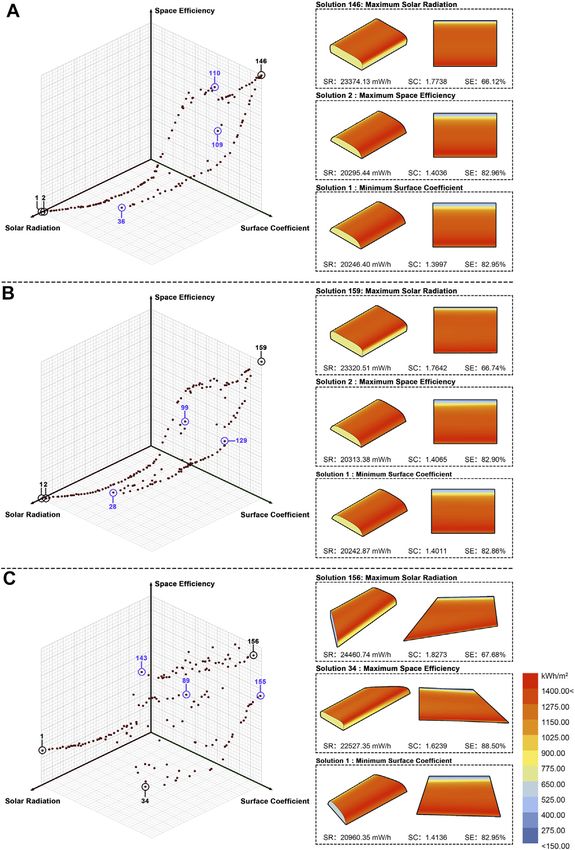
Zhang et al.                                                                                                Building Design Concerning Solar Energy

 FIGURE 2 | The “white box” design model.

Shao et al., 2014; Kim and Clayton, 2020; Xu et al., 2021), the                In addition, the energy performance and space utilization of
selection and operation of mechanical systems (Han et al., 2013;            buildings must also be considered in the building shape design
Penna et al., 2015) and the building shape. Because it is difficult to       (Kämpf et al., 2010; Tronchin et al., 2016; Talaei et al., 2021).
describe a single variable, the relevant research always uses the           Energy performance requires building shape to be adapted to
shape type (Tuhus-Dubrow and Krarti, 2010; Bichiou and Krarti,              the climate and avoid excessive heat exchange between the
2011; Ciardiello et al., 2020), orientation (Nguyen and Reiter,             building and the external environment, and space utilization
2014; Xu et al., 2015; Yu et al., 2015) and aspect ratio (Ramallo-          demands that the building meet the functional requirements
González and Coley, 2014; Xu et al., 2015) as variables; however,           and, on this basis, minimize the waste of space. Although it is
Yi et al. pointed out that most studies are limited to simple               ideal to achieve the above three objectives simultaneously, they
geometries, and complex forms can be explored through their                 often conflict with one another in actual design practice and
proposed hierarchical node control method (Yi and Malkawi,                  are thus difficult to achieve simultaneously, which is a problem
2009), which provides the basis for the parameterized node-based            that is especially prominent in large-space buildings with a
model in this paper. Based on existing research, the contributions          large number of free forms. Increasing solar energy acquisition
of the present study include selecting large-space buildings as the         and expanding the solar interface of a building may cause
object, improving the energy efficiency of building by optimizing            excessive energy loss due to increases in the external surface of
the form, and taking the use of space into account.                         the building and result in wasted space. Tightening a building
    In this work, solar radiation gain is taken as the primary              to save energy may lead to limited access to sunlight or space
objective for the shape optimization of large-space buildings,              use constraints, so these three objectives must be balanced. In
because the active use of solar energy as a clean energy source can         addition to the objectives described above, secondary
effectively alleviate the problem of high energy consumption in             indicators such as the area, space volume, and height of a
large-space buildings. First, such buildings have large and                 building are also considered by the designer and need to be
relatively flat roofs that can be used as an excellent solar                 controlled in the design. Therefore, the issues that need to be
collector. In addition, these roofs have access to adequate                 considered in the shape optimization of large-space buildings
sunlight, and photothermal and photovoltaic technology can                  in the early design stage are quite complex and require a high
be used to convert solar energy into thermal energy or                      efficiency in the generation, selection, and iteration of
electricity for direct use in buildings. Second, sufficient                  concepts.
sunlight creates good conditions for natural lighting, and                     In this study, we propose a multi-objective genetic
reasonable lighting port designs can effectively reduce the                 algorithm (MOGA)-based method for the shape
lighting energy consumption of buildings, which is an                       optimization of large-space buildings. This method can
important part of building energy consumption. China’s                      quickly generate a large number of different shape concepts,
five primary solar radiation zone systems, established by                    automatically quantify and analyze the solar gain, energy
Jiang etc. in 2021, show that, with the exception of the                    performance, and space utilization of each concept, select
relatively low resource potential of Area V (mainly in                      concepts with better performance, further improve their
Sichuan Basin), most regions of China have good solar                       performance through iteration, and ultimately output and
energy potential, and it is feasible to collect solar energy                visualize the optimization results to provide a basis for the
through buildings (Jiang et al., 2021).                                     selection of the final concept by the designer (Raphael, 2011).

Frontiers in Energy Research | www.frontiersin.org                      3                                November 2021 | Volume 9 | Article 744974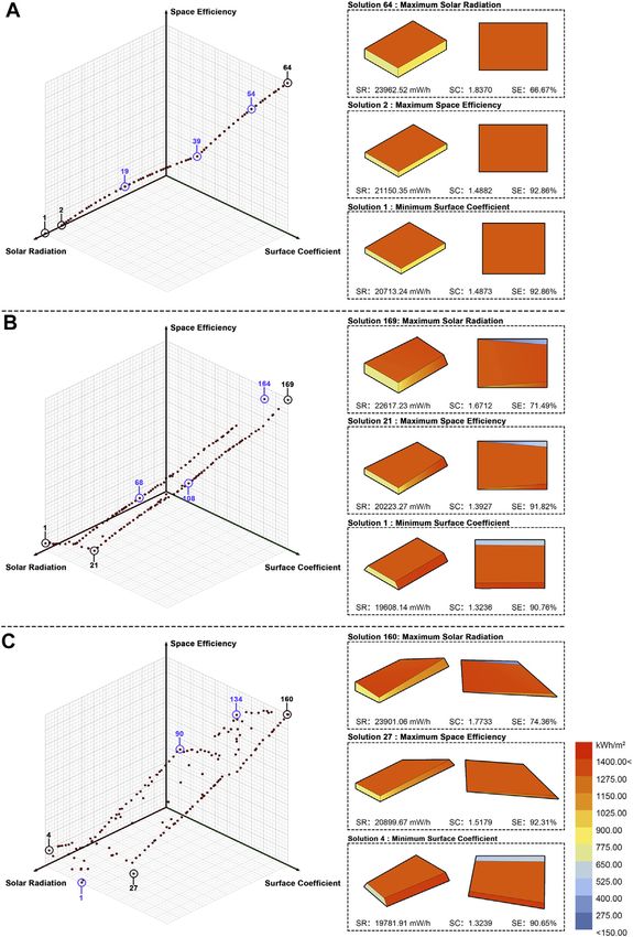
Zhang et al.                                                                                              Building Design Concerning Solar Energy

 FIGURE 3 | The “Modeling-Calculation-Optimization” process.

METHODOLOGY                                                                 shape control nodes (hereafter referred to as nodes) as
                                                                            variables to generate and manipulate the building shape
The method is based on the “Modeling-Calculation-                           (Jin and Jeong, 2013; Jin and Jeong, 2014).
Optimization” process and includes three steps, as shown in              3) Setting of constraints. Constraints define the range of change
Figure 3. First, a parametric shape model defined by the “core               in variables and may originate from functional requirements,
space” is constructed considering the large-space building                  design requirements, the intentions of the designer, and
characteristics. Second, by weighing the speed and accuracy                 standard specifications. In this step, the abovementioned
requirements in the early design stage, solar radiation gain,               conditions need to be concretized into numerical
energy performance, and space utilization are set as key                    constraints on node variables, which are specifically
indicators (Chang et al., 2019), and the corresponding                      expressed as the movable range of nodes in three-
calculation modules are developed to analyze the three key                  dimensional (3D) space.
aspects of performance quickly and quantitatively. Finally, the
MOGA (Wright et al., 2002; Wang et al., 2005a; Wang et al.,                  The shape variable definition and the constraint setting of the
2005b; Zhu et al., 2020) and the Pareto Frontier are applied to          shape model are shown in Figure 4. The building shape can be
achieve multi-performance optimization and visualize the results         summarized as a spatial structure formed by a number of nodes
of the early concepts (Tuhus-Dubrow and Krarti, 2010; Yi, 2019).         connected to each other in a specific order. This structure
                                                                         expresses the generation rules and evolution pattern of the
Parametric Building Shape Modeling                                       shape, and changing the position of the nodes alters the shape
In the early design stage, building shape modeling should not be         accordingly, thus controlling the change in shape (Negendahl,
overly limited to details such as the window form, material, and         2014). As shown in Figure 4A, the displacement of a node along
color but should use variables that are as simple as possible to         any direction can be decomposed into movements along the X-,
enable the building shape to transform freely within the                 Y-, and Z-axes, as Ax, Ay and Az, respectively. Therefore, a freely
constraints to explore a greater number of shape possibilities           movable node needs to be expressed by three variables, but when
and thereby provide the designer with a broader range of choices         the movement of the node along an axis is constrained, the
(Ourghi et al., 2007). Parametric shape modeling includes three          number of variables decreases. For example, in Figure 4B, node A
steps:                                                                   is located in the XY-plane and cannot move along the Z-axis, so
                                                                         its displacement is determined by the X and Y variables only;
1) Analysis of design requirements. In the early design stage, the       node A in Figure 4C follows node B along the Y-axis, so its
   geographic location, site environment, and climatic                   position can be described by the X and Z variables only; and the
   conditions of the building should be considered in detail to          movement of node A in Figure 4D depends on node B
   lay the foundation and precondition for the subsequent steps.         completely, so it has the same variables as node B, i.e., no new
2) Definition of shape variables. The variables in this study             variables are needed to describe its displacement.
   specifically refer to the independent variables that control               The building shape model with nodes as variables features the
   the generation of the building shape (Wang et al., 2006). The         following advantages: 1) the shape can be accurately manipulated
   designer can adjust the input values to change the building           by nodal displacements, which is especially suitable for generating
   shape. In previous studies, architectural variables such as the       and controlling nonlinear shapes; 2) the degree of freedom of
   orientation, area, story height, and story number have been           shape change can be altered by imposing constraints on the
   used to control the shape, and the pattern of shape change has        nodes, and the change interval of the shape can be controlled as
   been limited by the types of variables. To exercise a sufficient       needed; and 3) the variables are all nodal displacements, which
   degree of freedom for the shape to change, this study starts          are of the same type, share the same units, and can be concisely
   with the more essential shape generation rules and uses the           expressed and easily calculated.

Frontiers in Energy Research | www.frontiersin.org                   4                                 November 2021 | Volume 9 | Article 744974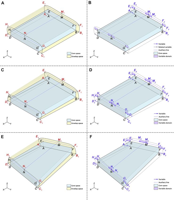
Zhang et al.                                                                                                            Building Design Concerning Solar Energy

 FIGURE 4 | The number of node variables changes under the constraint: (A) Independent movement of node A; (B) Node A in XY-plane cannot move along the
 Z-axis; (C) Node A follows node B along the Y-axis; (D) Movement of Node A depends on node B completely in 3 dimensions.

   The shape of a large-space building is defined by its inner core                Solar Radiation Gain
space and outer envelope enclosure. The core space is the space                   The solar gain of a building can be characterized by the annual
within the building that assumes the main use function, and its                   solar radiation gain at the surface of the building (Angelis-
size and shape are determined by the building function, not                       Dimakis et al., 2011), and its data can be obtained through
necessarily with clear physical boundaries. The envelope                          solar radiation simulations (Perez et al., 1990). To ensure the
enclosure is the outer interface of the building (Oral and                        accuracy and efficiency of the simulation, the Ladybug tool, based
Yilmaz, 2002) and can be understood as a “skin layer” that                        on the Grasshopper platform, was used in this study to calculate
wraps around the core space, with its form determined and                         the solar radiation gain (Roudsari and Pak, 2013). Ladybug
influenced by the core space. Therefore, the shape model of a                      simulates solar radiation using a Climate-Based Daylight
large-space building is actually a two-level node control system, in              Modeling (CBDM) method, which extracts area-specific
which the nodes constituting the core space are called core nodes                 meteorological data from EnergyPlus weather files (.epw) as
and their spatial positions are described by core variables, while                the basis for the simulation. The solar radiation function in
the nodes constituting the envelope enclosure are called envelope                 Ladybug uses the cumulative sky approach to calculate the
nodes and are described by envelope variables, which are defined                   amount of radiation for the Tregenza sky dome (Robinson
and constrained by core variables and change with them.                           and Stone, 2004). The total solar radiation incident on the test
                                                                                  model and the amount at each test point on the surfaces are
Calculation of Key Objectives                                                     accumulated, and the results are displayed on a multicolor user
In the early design stage, the objectives of the solar gain, energy               interface. This method has proven reliable in many studies (Yi
performance, and space utilization of the shape of a large-space                  and Kim, 2015; Freitas et al., 2020; Kharvari, 2020).
building are selected according to two principles: first, they are
representative and capable of summarizing and describing the                      Energy Performance
corresponding building performance in a general and accurate                      In general, energy consumption must be simulated to measure the
manner; second, they enable a high computational efficiency, do                    energy efficiency of a building. However, high-precision annual
not require a large consumption of time or computational                          simulations not only consume large amounts of time and
resources, and satisfy the need for performance analysis of a                     computational resources but also require detailed and accurate
large number of concepts in the early design stage.                               simulation parameters, which are difficult to determine in the

Frontiers in Energy Research | www.frontiersin.org                            5                                      November 2021 | Volume 9 | Article 744974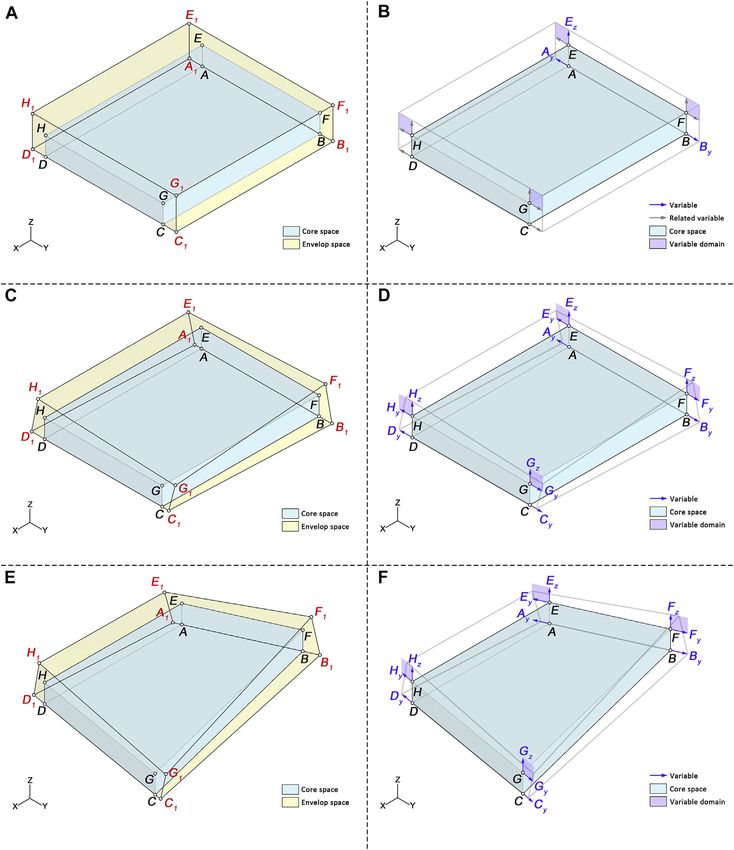
Zhang et al.                                                                                                     Building Design Concerning Solar Energy

early design stage. Therefore, an effective research approach is to            according to their performances and visualize them to provide a
select indicators that show significant correlations between the                basis for the designer to select the final solution to be
building shape and energy consumption (Jedrzejuk and Marks,                    implemented. The objective function of shape optimization
2002). Relevant studies have used a variety of indicators such as              can be written as follows:
the shape coefficient (Menezo et al., 2001), the building
                                                                                              min f(x)  f1 (x), f2 (x), f3 (x)                   (4)
corresponding area coefficient (Zhao and Hu, 2012), and the                                     x∈X
thermal shape coefficient (Lin and Li, 2016). Based on the latest               where
research results, the surface coefficient was used as the core
indicator in this study (Wang et al., 2020). The surface                                        f1 (x)  −SR                                        (5)
coefficient is defined as the ratio of the exterior surface area of                               f2 (x)  SC  F0 /S                                 (6)
the building in contact with the air to the building area; that is,                                               n (Vu )i × ri
                                                                                                f3 (x)  −SE  − i1                                (7)
                                  SC  F0 /S                        (1)                                               V0

where SC is the surface coefficient, F0 is the exterior surface area               Optimization problems are generally expressed as minimum
of the building, and S is the bottom surface area of the building.             value problems. Therefore, the purpose of shape optimization is
These two values can be obtained directly from a parametric                    to find the solutions that achieve the minimum values of the three
model. Studies have shown that the dimensionless surface                       objectives. f1 (x) is the total sunlight obtained by the building,
coefficient has a significant linear relationship with the energy                f2 (x) is the surface area coefficient of the building, f3 (x) is the
consumption per unit area of the building and can accurately                   spatial efficiency of the building. Because larger total sunlight and
reflect the correlation between the building shape and energy                   spatial efficiency values are better, the results of f1 (x) and f3 (x)
consumption.                                                                   are multiplied by -1 to minimize the function from maximization.
                                                                                  A variety of optimization algorithms, such as the genetic
Space Utilization                                                              algorithm (GA) (Ouarghi and Krarti, 2006), the sensitivity
Inappropriate height, location, and shape values for a building                vector algorithm (SVA) (Wang and Zhao, 2021), and the
can lead to inefficient space utilization, resulting in a waste of              Manta Ray Foraging Optimization algorithm (MRFOA) (Feng
space and additional energy and material consumption (Coakley                  et al., 2021), have been used for building shape optimization. In
et al., 2014). In our previous study (Zhang et al., 2016), the                 this study, the Pareto optimization method was used for shape
concept of space efficiency (SE) was proposed to measure the                    optimization. This method balances multiple objectives by
extent of utilization of the interior space of a building:                     finding nondominated solutions, also known as Pareto
                                                                               solutions. These solutions are not dominated by other
                                 SE  Vu /V0                        (2)        solutions in the solution space. The set of nondominated
where E is the space efficiency, Vu is the volume of available space,           solutions is called the Pareto Frontier, and each optimized
and V0 is the total volume of the interior space of the building.              solution has a particular performance benefit and achieves a
Large-space buildings are characterized by zoning use and time-                certain optimal tradeoff among the multiple objectives. This
sharing operation, and the extent of use of each space zone varies             method is particularly suitable for complex optimization
significantly over time. Therefore, the utilization rate is                     problems such as the one involved in this study.
introduced to modify Eq. 2. The utilization rate refers to the                    An optimization tool called Octopus, a Grasshopper plug-in,
percentage of time in hours that a specific space region is put into            was used to carry out the optimization. Octopus is a MOGA tool
use relative to the total operating time of the building throughout            based on the principle of evolution and can achieve the optimal
the year. The utilization rate is 100% for the space region that is            tradeoff of multiple optimization objectives through a multi-
put into use during the entire operation period of the building, 0%            objective optimization process. Octopus generates the set of
for the space region that is never used, 50% for the space region              optimized solutions for each generation in the form of a
that is used for half of the operation period, and so on. Then, SE             Pareto Frontier and displays the form and key indicator
can be written as                                                              information of each solution to monitor and control the
                                                                               optimization process. In addition, Octopus can record various
                                   ni1 (Vu )i × ri                           types of secondary indicator information of the solution to
                            SE                                     (3)        provide a basis for the designer to choose the final
                                          V0
                                                                               optimization solution.
where n is the number of zones in the large space, i is the zoning
ID, and ri is the utilization rate of the ith zone. These values can all
be calculated using a parametric model.                                        CASE STUDY
MOGA Optimization                                                              Case Overview
Shape optimization can be divided into two steps. The first step is             To verify this method, a large-space exhibition hall in Shenyang,
to find the optimized shapes that perform well with respect to the              China, is used as a case study in this work. Shenyang is in a cold
three objectives and gather them into an optimized solution set.               region of China and is a typical winter city. The building design
The second step is to sort the shapes in the optimized solution set            considers the reception of sufficient sunlight and minimization of

Frontiers in Energy Research | www.frontiersin.org                         6                                  November 2021 | Volume 9 | Article 744974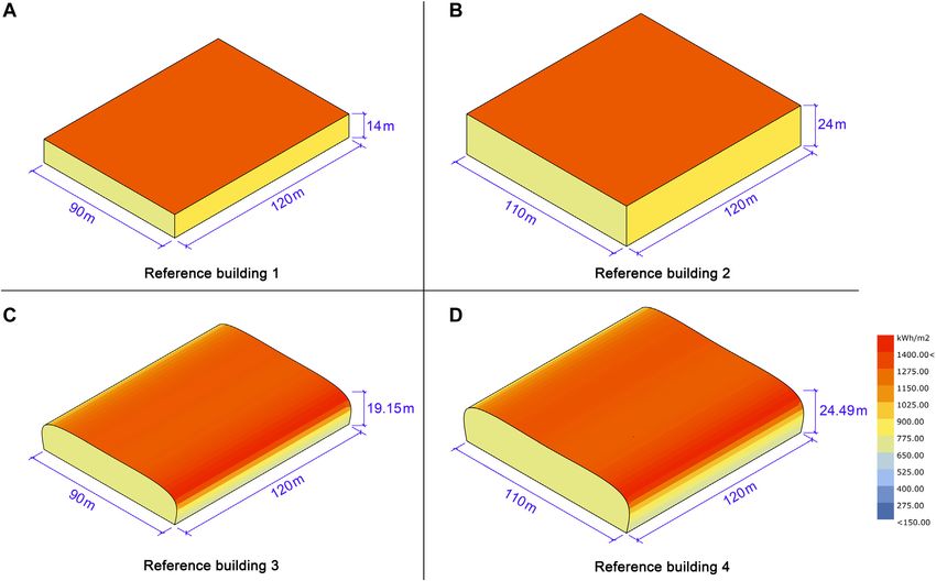
Zhang et al. Building Design Concerning Solar Energy
FIGURE 5 | The number of node variable changes under the constraint.
with a clear height greater than 2.1 m but less than 12 m (e.g.,
zone B or C) is available 70% of the time (i.e., utilization rate
70%). A space with a clear height that does not meet the use
requirements, i.e., less than 2.1 m (e.g., zone E), greater than 20 m
(e.g., zone G), or with a shape that does not meet the use
requirements (e.g., zone F, which has a roof area larger than
the corresponding floor area), has a utilization rate of 0.
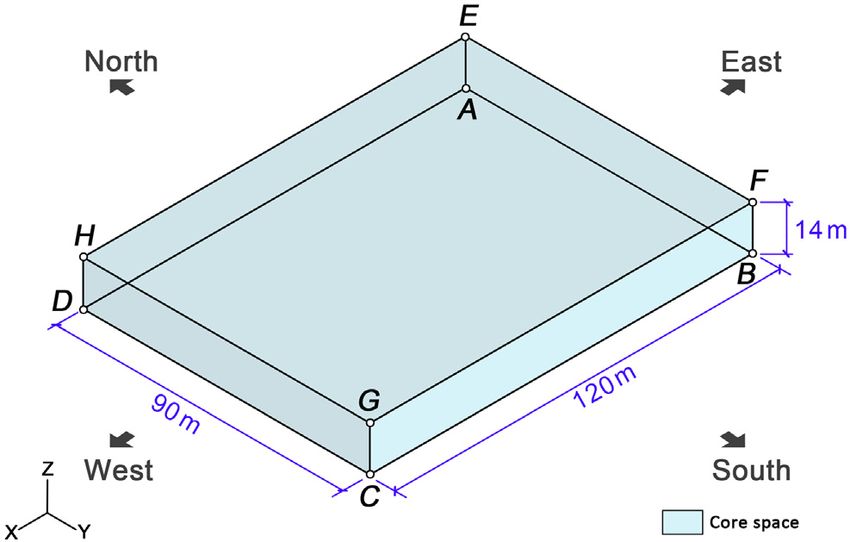
Shape Modeling
Core Space Modeling
According to the design requirements, the core space is initially
box-shaped with a length of 120 m, a width of 90 m, and a height
of 14 m, as shown in Figure 6. The bottom nodes and top nodes
are labeled clockwise as A-D and E-H, respectively, with edges
BC, AD, AB, and CD facing south, north, east, and west,
FIGURE 6 | The core space and its variable information.
respectively. Since the height of the space remains constant at
14 m, nodes E-H can only move along the horizontal direction,
and hence, the change in the core space is reflected in the change
in the form of plane. In this work, two planar forms commonly
the exterior surface area of the building to reduce energy
used in exhibition halls—rectangular plane and convex
consumption as important sustainable design goals. Climate
quadrilateral plane—are selected for comparative study.
information for Shenyang is available from the website
In the rectangular plane shown in Figure 7A, the three
(https://www.energyplus.net/weather).
adjacent edges that pass through any node are perpendicular
The exhibition hall is arranged in the north-south direction to each other. Node A is set as the origin (the same below), and
and has the following design requirements: 1) the large core space node D is allowed to move along the X-axis as node variable Dx.
with an exhibition function has the basic size of 120 m × 90 m × When node D moves, nodes B and C will move with it to ensure
14 m and a variable planar form with a total area of not less than that the adjacent edges remain perpendicular to each other under
10,800 m2; 2) the total building height is not less than 14 m and the condition of a constant area. Assuming that D1 and D2 are the
not greater than 24 m; and 3) in addition to the core space, there is endpoints of D moving along the X-axis, when node D moves to
a 10-m space at both the north and south sides of the building for D1, the corresponding node C will move to C1, and when node D
shape adjustment. These design requirements can be converted moves to D2, node C will then move to C2. Therefore, only one
into constraints on shape variables. The actual utilization of the variable Dx is needed to control the change in the plane of the core
building space requires field observation. Since this work aims to space. In this work, the D1 and D2 directions are set to be positive
verify the feasibility of the method, the problem is simplified by and negative directions, respectively, and this core space model is
assuming the utilization rate of each space zone based on the denoted as C1.
height and location. According to the standard requirement for The case of the convex quadrilateral plane as shown in
the height of an exhibition hall space, as shown in the section view Figure 7B becomes complex. Since there is no restriction that
in Figure 5, it is assumed that a space with a clear height of 12 m adjacent edges are perpendicular to each other, three additional
(e.g., zone A) can be fully utilized (i.e., utilization rate 100%), a variables in addition to Dx are needed to ensure that the planar
space with a clear height greater than 12 m and less than or equal area remains unchanged when the plane shape changes. In this
to 20 m (e.g., zone D) has a utilization rate of 50%, and a space work, the change in plane shape is controlled by setting the offset
Frontiers in Energy Research | www.frontiersin.org 7 November 2021 | Volume 9 | Article 744974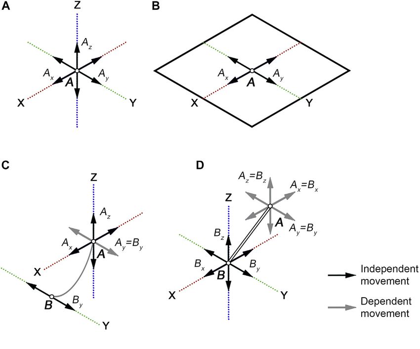
Zhang et al.                                                                                                          Building Design Concerning Solar Energy

 FIGURE 7 | Control nodes and variables of the core space: (A) rectangular plane; (B) convex quadrilateral plane.

angle: 1) the angle between the edge CD and the Y-axis is set as                        Figure 8B, because the adjacent faces are perpendicular to
∠α, with clockwise and counterclockwise rotations being positive                        each other, nodes D, H, and E move together with node A
and negative, respectively; 2) the angle between the edge AB and                        along the Y-axis with the same displacement as Ay; C, F, and G
the X-axis is set as ∠ β, which is the mirror image of ∠α, with                         move together with B along the Y-axis with the same
clockwise and counterclockwise rotations being negative and                             displacement as By; and F, G, and H move together with E
positive, respectively; and 3) the angle between the edge BC                            along the Z-axis with the same displacement as Ez. Thus, the
and the X-axis as ∠γ, with clockwise and counterclockwise                               form change of S1 can be controlled by envelope variables Ay,
rotations being negative and positive, respectively. This core                          By, and Ez and the core variable Dx.
space model is denoted as C2.                                                        2) Shape2 (S2) is also based on C1 as is S1, but there is no
                                                                                        restriction that adjacent edges are perpendicular to each other.
Envelope Modeling                                                                       As shown in Figure 8C, nodes A-H can independently move
The final shape of the building can be generated by constructing                         to the corresponding positions A1-H1, and in this case there
the envelope variable system based on core spaces C1 and C2. The                        can be various angles between adjacent edges. Figure 8D
envelope nodes can be regarded as those obtained by moving the                          shows that nodes A-D can all move freely along the Y-axis as
core nodes A-H, so the corresponding envelope nodes are set as                          the corresponding variables Ay-Dy; nodes E-H can move
A1-H1. Since the envelope nodes of the building can only move                           freely along the Y-axis and Z-axis, with the corresponding
outside the core space, the displacements of the nodes away from                        variables denoted as Ey-Hy and Ez-Hz, respectively. In this
the core space along the X-, Y-, and Z-axes are defined as positive,                     case, 12 envelope variables and one core variable Dx are
which can simplify the description and calculation of the shape                         required to control the form change of S2.
variables.                                                                           3) As shown in Figure 8E, Shape3 (S3) is based on C2, and its
   In this work, six typical large-space shapes are selected as the                     nodes are similar to those of S2. A-H can move independently
optimization alternatives (S1–S6). All nodes in S1–S3 are                               to the corresponding positions A1-H1, and there can be a
connected by straight lines and are thus denoted as straight-                           variety of angles between adjacent edges. The envelope
edge shapes (Figure 8). The nodes on the east and west sides in                         variables for S3 shown in Figure 8F are the same as those
the middle of S4–S6 are passed through by curves, so these three                        for S2, and these 12 envelope variables and four core variables
are curved-edge shapes (Figure 9). These curves are generated                           of C2, totaling 16 variables, are needed to control the form
using the “interpolate curve” command in Rhinoceros software,                           change of S3.
with degree and weight set to 3 and 1, respectively, to ensure that                  4) Based on C1, Shape4 (S4) is a curved-edge shape with
there is one and only one curve passing through these nodes. It                         symmetrical east and west sides and is integrated by the
should be noted that the east and west façades of these six shapes                      top surface of the building and the north and south
are all perpendicular to the ground for two reasons. First, in                          façades. The envelope nodes on the east and west sides of
building design, traffic space is usually set up on the short-edge                       the building are symmetrically positioned and each
side of the exhibition hall or along connections with other                             intersected by separate curves with the same trend. To
exhibition halls, and the vertical façades are conducive to                             control the building height and the change trend of the
space arrangement. Second, compared to the roof and south                               curved-edge shape, a ridgeline is set at the roof of the
façades, changes in angle of the east and west façades have little                      building with two endpoints M1 and N1, which are
impact on solar energy capture, and hence, setting the two façades                      obtained by moving the midpoint M of the line connecting
as vertical helps simplify the problem. Details of the six shapes                       nodes E1 and F1 and the midpoint N of the line connecting
and their variables are as follows.                                                     nodes H1 and G1 along the Y- and Z-axes, respectively, as
                                                                                        shown in Figure 9A. Using the “interpolate curve” command
1) Shape1 (S1) is a box shape, as shown in Figure 8A. It has C1 as                      (with the degree of the curves set to 3 and the weights set to 1,
   the base, and the three adjacent edges passing through any                           the same below), two curves are obtained by connecting A1,
   envelope node are perpendicular to each other. As shown in                           E1, M1, F1, and B1 to D1, H1, N1, G1, and C1, respectively, to

Frontiers in Energy Research | www.frontiersin.org                               8                                  November 2021 | Volume 9 | Article 744974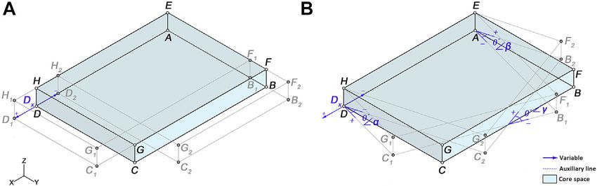
Zhang et al.                                                                                                              Building Design Concerning Solar Energy

 FIGURE 8 | Node systems and envelope variables of straight-edge shapes: (A) node systems of S1; (B) envelope variables of S1; (C) node systems of S2; (D)
 envelope variables of S2; (E) node systems of S3; (F) envelope variables of S3.

   generate the building envelope. Regarding envelope variables                        any of the positions A1-N1, the number of envelope variables
   of S4 shown in Figure 9B, due to the east-west symmetry of                          is doubled compared to that of S4. As seen in Figures 9A,D
   the shape, the displacements of nodes C, D, H, G, and N are                         total of 16 envelope variables and one core variable Dx are
   the same as those of nodes B, A, E, M, and F, respectively, so S4                   needed to control the shape change of S5.
   can be described by eight envelope variables (Ay, By, Ey, Ez, Fy,
   Fz, My, and Mz) and the core variable Dx.                                        6) Shape6 (S6) takes C2 as the core space, as shown in Figure 9E,
5) Shape5 (S5) is based on C1 and is a curved-edge shape like S4,                      and nodes A-N each can move to any of the positions A1-N1.
   except that the east and west sides need not be symmetrical, as                     Figure 9F shows that S6 has 16 envelope variables, which are
   shown in Figure 9C. In addition, nodes A-N can each move to                         the same as those of S5, but its core variables are increased to

Frontiers in Energy Research | www.frontiersin.org                              9                                      November 2021 | Volume 9 | Article 744974
Zhang et al.                                                                                                             Building Design Concerning Solar Energy

 FIGURE 9 | Node systems and envelope variables of curved-edge shapes: (A) node systems of S4; (B) envelope variables of S4; (C) node systems of S5; (D)
 envelope variables of S5; (E) node systems of S6; (F) envelope variables of S6.

    four, as determined by C2. Therefore, a total of 20 variables are              Values of Variables
    needed to describe its form change.                                            The value range and accuracy of the variables directly affect the
                                                                                   complexity of the optimization. The optimization efficiency can
   The six shapes described above are typical of the shapes                        be improved by setting reasonable upper and lower bounds and
commonly used in large-space exhibition halls. These shapes                        step sizes for the variables. Considering the complexity of the
range from simple to complex, with increasing numbers of node                      optimization in this case, the variables are defined as follows: 1)
variables. The information on the six shapes is summarized in                      For the two core spaces C1 and C2, the range of Dx is set to be
Table 1.                                                                           between −20 and 20 m (inclusive), with a step size of 0.1 m. 2) In

Frontiers in Energy Research | www.frontiersin.org                            10                                      November 2021 | Volume 9 | Article 744974
Zhang et al. Building Design Concerning Solar Energy
TABLE 1 | Summary of the six shapes.
S1 S2 S3 S4 S5 S6
Number of nodes 8 8 8 10 10 10
Relation type Linear Linear Linear Curve Curve Curve
Core plan form Rectangle Rectangle Convex quadrilateral Rectangle Rectangle Convex quadrilateral
South and north façade Planar Surface Surface Surface Surface Surface
East and west facade Planar Planar Planar Planar Planar Planar
Roof Planar Surface Surface Surface Surface Surface
Number of core variables 1 1 4 1 1 4
Number of envelop variables 3 12 12 8 16 16
Total number of variables 4 13 16 9 17 20
TABLE 2 | Domains of the shape variables.
S1 S2 S3 S4 S5 S6
Min Max Min Max Min Max Min Max Min Max Min Max
Core Variables Dx −20 20 −20 20 −20 20 −20 20 −20 20 −20 20
∠α — — — — −15 15 — — — — −15 15
∠β — — — — −15 15 — — — — −15 15
∠γ — — — — −20 20 — — — — −20 20
Envelope Variables Ay 0 10 0 10 0 10 0 10 0 10 0 10
By 0 10 0 10 0 10 0 10 0 10 0 10
Cy — — 0 10 0 10 — — 0 10 0 10
Dy — — 0 10 0 10 — — 0 10 0 10
Ey — — 0 10 0 10 0 10 0 10 0 10
Fy — — 0 10 0 10 0 10 0 10 0 10
Gy — — 0 10 0 10 — — 0 10 0 10
Hy — — 0 10 0 10 — — 0 10 0 10
Ez 0 10 0 10 0 10 0 5 0 5 0 5
Fz — — 0 10 0 10 0 5 0 5 0 5
Gz — — 0 10 0 10 — — 0 5 0 5
Hz — — 0 10 0 10 — — 0 5 0 5
My — — — — — — −10 10 −10 10 −10 10
Ny — — — — — — — — −10 10 −10 10
Mz — — — — — — 5 10 5 10 5 10
Nz — — — — — — — — 5 10 5 10
C2, ∠α and ∠β are allowed to change within ±15° and ∠γ to Grasshopper plug-in Ladybug, SC and SE are calculated by a
change within ±20°, with a step size of 1°. 3) The values of all program written in Grasshopper, and the secondary indicators
variables of each node in S1–S3 and variables of each node in can be obtained by direct query in Grasshopper.
S4–S6 on the X- and Y-axes can range from 0 to 10 m (inclusive),
with a step size of 0.1 m. 4) Nodes E, F, G, H, M, and N in S4–S6 Reference buildings
can range between 0 and 5 m along the Z-axis, with the distance To verify the effectiveness of this optimization method, reference
from nodes M and N to the core space ensured to be between 0 buildings for comparative study are defined with the following
and 10 m and the step size of the above variables set to 0.1 m, rules: 1) corresponding reference buildings are set for straight-
which is consistent with that for S1–S3. Finally, 5) in S4–S6, the edge shapes and curved-edge shapes; 2) the reference buildings
horizontal movement of nodes M and N is set to range between are modeled after the baseline straight-edge shape S1 and the
−10 and 10 m, with a step size of 0.1 m. Details of the variables are curved-edge shape S4, respectively, and the upper and lower
shown in Table 2. bounds of the node variables except Dx are removed to evaluate
the performance of building shapes under extreme conditions.
Key Objective Calculations Therefore, there are a total of four reference buildings,
In this case, solar radiation (SR), the surface coefficient (SC), and numbered 1–4, with the minimum and maximum values of
space efficiency (SE) are selected as the key objectives for node variables of S1 selected for reference buildings 1 and 2,
optimization, where larger SR and SE values and smaller SC respectively, and the minimum and maximum values of node
values are better. In addition, the building area, volume, and variables of S4 selected for reference buildings 3 and 4,
height are selected as secondary indicators to provide a basis for respectively. After the simulation, the shapes and solar
the designers to select solutions. SR is calculated using the radiation distributions of the reference buildings are shown
Frontiers in Energy Research | www.frontiersin.org 11 November 2021 | Volume 9 | Article 744974Zhang et al. Building Design Concerning Solar Energy
FIGURE 10 | The shapes and solar radiation distributions of the reference buildings: (A) Reference building 1; (B) Reference building 2; (C) Reference building 3; (D)
Reference building 4.
TABLE 3 | Variables and performance of the reference buildings.
Reference building 1 Reference building 2 Reference building 3 Reference building 4
Variables Dx 0 0 0 0
Ay 0 10 0 0
By 0 10 0 0
Ey 0 10 0 0
Fy — — 0 0
Ez — — 0 5
Fz — — 0 5
My — — 0 0
Mz — — 5 10
Key objectives Solar 17,147.99 23,232.45 17,823.06 22,749.33
Radiation (MWh)
Surface 1.5444 1.8364 1.66 1.7834
Coefficient
Space 92.8571 66.6667 81.1591 65.9539
Efficiency (%)
Secondary indicator Area (m2) 10,800 13,200 10,800 13,200
Volume (m3) 16,680 24,240 17,927.66 23,540.87
Height (m) 14 24 19.15 24.49
Frontiers in Energy Research | www.frontiersin.org 12 November 2021 | Volume 9 | Article 744974Zhang et al. Building Design Concerning Solar Energy
FIGURE 11 | Pareto Frontier of S1 and the building shapes of its optimal solutions: (A) S1; (B) S2; (C) S3.
in Figure 10, and the values of their respective variables, core RESULTS AND DISCUSSION
indicators (“Objectives”), and secondary indicators are
presented in Table 3. The optimization method proposed in this work can achieve
nondominated solutions for the optimized tradeoff among three
key objectives, and the optimization results can be used to
MOGA settings support the early-stage design of large-space building shapes
For this case, the following MOGA parameter values were set: in three ways: 1) By visualizing the Pareto Frontier, the
the population size 50, maximum generations 100, crossover distribution pattern of nondominated solutions can be
rate 0.8, mutation probability 0.2, mutation rate 0.9 and presented and the information on key objectives distribution
elitism 0.5. The optimization was performed on a computer displayed. 2) The performance characteristics of the optimized
with Windows 10 (16 core 3.5 GHz processor, 8G RAM), and the shapes can be investigated through a horizontal comparison of
total calculation required 120.4 h. The results are presented the optimized solutions for different shape types, and the
hereafter. performance improvement effect of the optimization can be
Frontiers in Energy Research | www.frontiersin.org 13 November 2021 | Volume 9 | Article 744974Zhang et al. Building Design Concerning Solar Energy
FIGURE 12 | Pareto Frontier of S1 and the building shapes of its optimal solutions: (A) S4; (B) S5; (C) S6.
verified by comparing the optimized shapes with reference remaining solutions achieves the optimal tradeoff among the
buildings. Finally, 3) analysis of the distribution of the shape three objectives, which is called a characteristic solution in this
variables in the optimized solutions facilitates both the discovery study and can be selected as the final scheme. The optimal
of typical shape characteristics of the optimized solutions and the solutions for single indicators are presented here, with their
potential identification of key variables affecting building positions in the Pareto Frontier, building shapes, sunlight
performance, which provides a reference for subsequent in- distributions, and key indicators shown in Figure 11. The
depth designs. other three random characteristic solutions of each shape are
also marked, and their key indicator values were also used in the
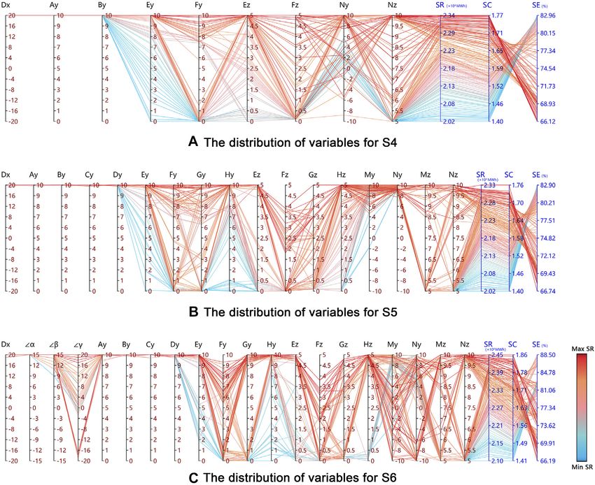
Pareto Frontier comparative analysis.
The Pareto Frontier for each of the six shapes in this case study
was generated after 100 iterations. Each point on the Pareto 1) Figure 11A shows the Pareto Frontier for S1, which has a total
Frontier is a nondominated solution. Except for the solution that of 63 nondominated solutions that are approximately
obtains the optimal value for a core indicator, each of the distributed in an arc. Solution 63 has the largest solar
Frontiers in Energy Research | www.frontiersin.org 14 November 2021 | Volume 9 | Article 744974Frontiers in Energy Research | www.frontiersin.org
Zhang et al.
TABLE 4 | Performance of S1-S3 characteristic solutions and comparison with reference buildings 1 and 2.
Solar radiation Surface coefficient Space efficiency Reference building 1 Reference building 2
(MWh) (%)
Solar radiation Surface coefficient Space efficiency Solar radiation Surface coefficient Space efficiency
improvement (%) improvement (%) improvement (%) improvement (%) improvement (%) improvement (%)
S1 Best SR 23,962.52 1.8370 66.67 39.74 −18.95 −28.20 3.14 −0.03 0.00
Best SC 20,713.24 1.4873 92.86 20.79 3.70 0.00 −10.84 19.01 39.29
Best SE 21,150.35 1.4882 92.86 23.34 3.64 0.00 −8.96 18.96 39.29
C19 21,937.75 1.5859 85.71 27.93 −5.57 −2.69 13.64 −7.70 28.56
C39 22,837.65 1.6626 81.58 33.18 −7.65 −12.14 −1.70 9.46 22.37
C54 23,512.57 1.7812 71.43 37.12 1.21 -15.33 3.01 −23.08 7.14
S2 Best SR 22,617.23 1.6712 71.49 31.89 −8.21 −23.01 −2.65 9.00 7.23
15
Best SC 19,608.14 1.3236 90.76 14.35 14.30 −2.26 −15.60 27.92 36.14
Best SE 20,223.27 1.3927 91.82 17.93 9.82 −1.12 −12.95 24.16 37.73
C68 20,941.85 1.4396 85.54 22.12 −9.86 6.79 21.61 −7.88 28.31
C108 21,512.78 1.5140 83.38 25.45 −7.40 1.97 17.56 −10.21 25.07
C164 22,401.30 1.6287 71.76 30.64 −5.46 −22.72 −3.58 11.31 7.64
S3 Best SR 23,901.06 1.7733 74.36 39.38 −14.82 −19.92 2.88 3.44 11.54
Best SC 19,781.91 1.3239 90.65 15.36 14.28 −2.38 −14.85 27.91 35.97
Best SE 20,899.67 1.5179 92.31 21.88 1.72 −0.59 −10.04 17.34 38.46
C1 19,673.43 1.4553 92.27 14.73 5.77 −0.63 −15.32 20.75 38.40
C90 22,441.31 1.5280 79.87 30.87 1.06 −13.99 −3.41 16.79 19.80
C134 23,248.34 1.6515 75.18 35.57 −6.93 −19.04 0.07 10.07 12.77
November 2021 | Volume 9 | Article 744974
Building Design Concerning Solar EnergyZhang et al. Building Design Concerning Solar Energy
radiation, 23,962.52 MWh; Solution 1 has the smallest surface Comparative Analysis of the Results
coefficient, 1.4870; and Solution 2 has the highest space The comparative analysis of the results includes a comparison of
efficiency, up to 92.86%. The two solutions are close to the optimized solutions among different shape types and
each other in the Pareto Frontier, indicating that the comparisons with the corresponding reference buildings.
surface coefficient and space efficiency are highly correlated The solar radiation, surface coefficient, and space efficiency
for S1. values for the extremal solutions and the remaining characteristic
2) The Pareto Frontier of S2 is shown in Figure 11B. There solutions of S1, S2, and S3 with straight edges, as well as the
are a total of 169 nondominated solutions, which are improvements relative to reference building 1 and reference
distributed in two curves. Solution 169 located at the building 2, are shown in Table 4. In terms of solar radiation,
top end of the curve on the right side has the highest each optimized shape shows a significant improvement over that
solar radiation, 22,617.23 MWh; Solution 1 has the for reference building 1. The solution with the greatest
smallest surface coefficient, 1.3236; and Solution 21 has improvement is the Best SR solution of S1, exhibiting an
the highest space efficiency, 91.82%. improvement of 39.74% in solar radiation accompanied by a
3) As shown in Figure 11C, the Pareto Frontier of S3 is more change of 18.95% in the surface coefficient and 28.20% in space
scattered than that of S2, and there are a total of 160 efficiency; and the solution with the smallest improvement is the
nondominated solutions, which are approximately Best SC solution of S2, with a 14.35% increase in solar radiation
distributed over a curved surface. Solution 160 at the top along with a 14.30% increase in the surface coefficient but a 2.26%
right end of the surface has the highest solar radiation, decrease in space efficiency, noting that the decrease is much
23,901.06 MWh; Solution 4 has the smallest surface smaller than the increases in the other two indicators. In contrast
coefficient, 1.3239; and Solution 27 has the highest space to reference building 2, which performs well in solar radiation,
efficiency, 92.31%. The rest of the characteristic solutions most of the nondominated solutions show a decrease in solar
each have their own shape characteristics and emphasized radiation but a significant improvement in the surface coefficient
indicators, which can meet the diverse preferences of and space efficiency. The solution with the largest reduction in
designers for shapes. solar radiation is the Best SC solution of S2, which shows a
4) The Pareto Frontier of S4 is shown in Figure 12A, which 15.60% decrease in solar radiation in exchange for a 27.92%
contains a total of 146 nondominated solutions distributed improvement in the surface coefficient and a 36.14%
approximately on two curves that converge at the upper right improvement in space efficiency. It is worth mentioning that
corner, where Solution 146 is located. This solution has the the best SR solution of S3 improves all three indicators by 2.88,
highest solar radiation, 23,374.13 MWh; Solution 1 has the 3.44, and 11.54%, respectively.
smallest surface coefficient, 1.3997; and Solution 2 has the The solar radiation, surface coefficient, and space efficiency of
highest space efficiency, 82.96%. Solutions 1 and 2 have very each nondominated solution of the curved-edge shapes S4, S5,
close values for each indicator and are located in the lower left and S6 and the improvements relative to reference buildings 3
corner of the Pareto Frontier. and 4 are shown in Table 5. The comparison with reference
building 3 shows that the solar radiation of each nondominated
5) Figure 12B shows that there are 159 nondominated solutions solution increases significantly, and the Best SR solution of S6
in the Pareto Frontier of S5, with a distribution similar to that improves solar radiation the most, by up to 37.24%, albeit
of S4. Specifically, the formed curves also converge at the top, accompanied by a 10.08% decrease in the surface coefficient
where Solution 159 is located. This solution features the and a 16.61% decrease in space efficiency. The best SC
highest solar radiation of 23,320.51 MWh; at the lower left solution of S5 has the smallest increase in solar radiation,
corner of the curves, Solution 1 has the smallest surface 13.58%, but its surface coefficient and space efficiency increase
coefficient of 1.4011 and Solution 2 the highest space by 15.60 and 2.10% respectively, indicating that the three
efficiency of 82.90%. A comprehensive comparison revealed indicators are all better than those of reference building 3.
that the characteristic solutions differ substantially in terms of Compared with reference building 4, some of the characteristic
each indicator and hence can be selected according to solutions show reductions in solar radiation in the range of
different needs. 0.98–11.02% but display significant improvements in the other
6) Three core variables are added to S6, which therefore has a two indicators, with the improvement in the surface coefficient in
significantly different planar shape. Figure 12C shows its the range of 8.94–21.52% and the improvement in the space
Pareto Frontier, which consists of a total of 156 efficiency between 13.31 and 34.18%; other characteristic
nondominated solutions distributed on a roughly curved solutions exhibit an improvement in solar radiation between
surface. Solution 156 has the highest solar radiation, 0.43 and 7.52%, and most of these solutions feature
24,460.74 MWh; Solution 1 has the smallest surface improvements in both the surface coefficient and space
coefficient, 1.4136; and Solution 34 has the highest space efficiency, achieving an overall improvement in the three
efficiency, up to 88.50%. The remaining characteristic indicators.
solutions differ significantly in terms of the shape, The distribution of all nondominated solutions of the six
indicators, and variable values, indicating a broad range of shapes are analyzed to verify the effectiveness of the
optimization solutions and a high variability in the results, optimization and provide a basis for selection in the early
which can meet diverse design needs. design stage. As seen in Figure 13A, all the nondominated
Frontiers in Energy Research | www.frontiersin.org 16 November 2021 | Volume 9 | Article 744974Frontiers in Energy Research | www.frontiersin.org
Zhang et al.
TABLE 5 | Performance of S4-S6 characteristic solutions and comparison with reference buildings 3 and 4.
Solar radiation Surface coefficient Space efficiency Reference building 3 Reference building 4
(MWh) (%)
Solar radiation Surface coefficient Space efficiency Solar radiation Surface coefficient Space efficiency
improvement (%) improvement (%) improvement (%) improvement (%) improvement (%) improvement (%)
S4 Best SR 23,374.13 1.7738 66.12 31.15 −6.86 −18.53 2.75 0.54 0.25
Best SC 20,246.40 1.3997 82.95 13.60 15.68 2.21 −11.00 21.52 25.77
Best SE 20,295.44 1.4036 82.96 13.87 15.45 2.22 −10.79 21.30 25.78
C36 21,419.03 1.5326 82.56 20.18 7.67 1.73 −5.85 14.06 25.18
C112 22,868.91 1.6857 73.46 28.31 −1.55 −9.49 0.53 5.48 11.38
C113 22,877.14 1.6742 68.26 28.36 −0.86 −15.89 0.56 6.12 3.50
S5 Best SR 23,320.51 1.7642 66.74 30.84 −6.28 −17.77 2.51 1.08 1.19
17
Best SC 20,242.87 1.4011 82.86 13.58 15.60 2.10 −11.02 21.44 25.63
Best SE 20,313.38 1.4065 82.90 13.97 15.27 2.15 −10.71 21.13 25.69
C28 21,340.01 1.5087 82.56 19.73 9.11 1.73 −6.19 15.40 25.18
C99 22,481.80 1.6116 74.73 26.14 2.92 −7.92 −1.18 9.63 13.31
C129 22,847.89 1.6982 76.34 28.19 −2.30 -5.94 0.43 4.78 15.75
S6 Best SR 24,460.74 1.8273 67.68 37.24 −10.08 −16.61 7.52 −2.46 2.62
Best SC 20,960.35 1.4136 82.95 17.60 14.84 2.21 −7.86 20.74 25.77
Best SE 22,527.35 1.6239 88.50 26.39 2.17 9.05 -0.98 8.94 34.18
C89 23,479.17 1.6784 74.72 31.73 −1.11 −7.93 3.21 5.89 13.29
C143 24,231.46 1.7818 66.19 35.96 −7.34 −18.44 6.52 0.09 0.36
C155 24,456.53 1.8554 73.83 37.22 −11.77 −9.03 7.50 −4.04 11.94
November 2021 | Volume 9 | Article 744974
Building Design Concerning Solar EnergyZhang et al. Building Design Concerning Solar Energy
buildings 2 and 4. In terms of the surface coefficient, as shown in
Figure 13B, most of the nondominated solutions of all six shapes
are better than the reference buildings, with S2 performing the
best and approximately 75% of the nondominated solutions
performing better than reference building 1, the best
performer for this indicator among the reference buildings.
Figure 13C shows that the space efficiencies of all optimized
solutions lie between that of reference building 1, the best
performer by this indicator, and reference building 4, the
worst performer by this indicator, with S1, S2, and S3
performing relatively well, indicating that the straight-edge
shapes have an advantage in space utilization. Among the
curved-edge shapes, S6 has a higher upper bound due to its
greater flexibility in shape change and better chance of achieving
higher space efficiency.
Variable Distribution Analysis
In this work, a parallel coordinates plot (PCP) is used to analyze
the distribution of shape variables of nondominated solutions.
PCP is a visualization method suitable for multidimensional data
and can reflect the distributional trends in data and relationships
among variables. Using this method, we can clarify the variable
value patterns of the optimized solutions and thereby discover the
common shape characteristics of the nondominated solutions
and identify the key variables affecting building performance,
which can provide a reference for subsequent in-depth design.
The variable distributions of straight- and curved-edge shapes are
shown in Figures 11,12, respectively, where the solutions with
different solar radiation gains are marked in different colors, as
noted in the legend.
1) The variable distribution of S1 in Figure 14A shows that Dx,
Ay, and By generally take their respective maximum values
with high consistency, indicating that the depth of the
building and the area of the south façade both tend to
increase in optimized shapes. In terms of optimization
objectives, solar radiation gain is positively correlated with
the surface coefficient and negatively correlated with space
efficiency. The solar radiation gain of the building depends
more on Ez, with a larger Ez leading to a higher solar radiation,
a greater surface coefficient, and a lower space efficiency.
Thus, Ez is the key variable for shape in this work and should
be given attention in the design.
2) Figure 14B shows the variable distribution of S2, which is
similar to that of S1, that is, Dx, Ay, By, Cy, and Dy tend to
choose their respective maximum values to maximize the
planar area and the south façade area. Similarly, solar
radiation gain is positively correlated with the surface
coefficient and negatively correlated with space efficiency.
FIGURE 13 | Performance distribution of six shapes and comparison Variables Hy, Ez, and Hz are strongly correlated with solar
with the reference buildings: (A) solar radiation; (B) surface coefficient; (C)
radiation, and the larger their values are, the greater the solar
space efficiency.
radiation gain of the building. Hence, these are key variables
that need to be addressed in design.
3) The variable distribution of S3 shown in Figure 14C is much
solutions of the six shapes are significantly better than reference more complex than those of S1 and S2. Specifically, the
buildings 1 and 3 in terms of solar radiation, and all the shapes distributions of the values of Dx, ∠α, ∠β, Ay, By, Cy, Dy,
except S2 have several optimized solutions better than reference and Hy of nondominated solutions are relatively concentrated,
Frontiers in Energy Research | www.frontiersin.org 18 November 2021 | Volume 9 | Article 744974You can also read