Bayesian Assessments of Aeroengine Performance
←
→
Page content transcription
If your browser does not render page correctly, please read the page content below
Bayesian Assessments of Aeroengine Performance∗
                                          Pranay Seshadri† , Andrew Duncan‡ , George Thorne§ , Geoffrey Parks¶,                    and   Mark Girolamik

                                         Abstract. Aeroengine performance is determined by temperature and pressure profiles along various axial
                                                   stations within an engine. Given limited sensor measurements along an axial station, we require
                                                   a statistically principled approach to inferring these profiles. In this paper, we detail a Bayesian
                                                   methodology for interpolating the spatial temperature or pressure profile at a single axial station
                                                   within an aeroengine. The profile is represented as a spatial Gaussian random field on an annulus,
                                                   with circumferential variations modelled using a Fourier basis and a square exponential kernel re-
                                                   spectively. In the scenario where precise frequencies comprising the temperature field are unknown,
                                                   we utilise a sparsity-promoting prior on the frequencies to encourage sparse representations. The
arXiv:2011.14698v1 [cs.CE] 30 Nov 2020

                                                   main quantity of interest, the spatial area average is readily obtained in closed form, and we demon-
                                                   strate how to naturally decompose the posterior uncertainty into terms characterising insufficient
                                                   sampling and sensor measurement error respectively. Finally, we demonstrate how this framework
                                                   can be employed to enable more tailored design of experiments.

                                         Key words. Gaussian random fields, sparsity promoting priors, Bayesian quadrature

                                         AMS subject classifications. 60G15, 51M35

                                             1. Introduction. Ensuring that aeroengines operate as efficiently as possible—so as to
                                         minimize their fuel consumption and carbon footprint—is a challenging task. The past decade
                                         has seen great strides in this respect: sustained aeroelastic, aerodynamic and aeroacoustic im-
                                         provements at both the component and system architecture level have yielded engine manufac-
                                         turers impressive efficiency gains, empowering cleaner flight. While overall engine efficiency is
                                         relatively well understood and is a function of fuel flow and thrust, it is the breakdown of this
                                         overall efficiency into key sub-system efficiencies that is the real challenge. These sub-systems
                                         include the low, intermediate and high pressure compressor and turbine components and the
                                         combustor. A solid understanding of the differences between expected and achieved sub-
                                         system performance informs engine manufacturers where they need to focus their attention
                                         to facilitate greater overall efficiency gains.
                                             One can interpret the computation of efficiency as the aggregation of an engine’s compos-
                                         ite pressures and temperatures taken at numerous measurement planes distributed across the
                                         engine. At each measurement plane, circumferentially positioned rakes—with one to seven ra-

                                            ∗
                                              Funded by Rolls-Royce plc. as part of the Engine Uncertainty Assessments Project.
                                            †
                                              Research Fellow, Department of Mathematics (Statistics Section), Imperial College London, London,
                                         U. K.; Group Leader, Data-Centric Engineering, The Alan Turing Institute, London, U. K. Email:
                                         p.seshadri@imperial.ac.uk; Web: www.psesh.com.
                                            ‡
                                              Lecturer, Data-Centric Engineering, Department of Mathematics (Statistics Section), Imperial College, London,
                                         U. K.; Group Leader, Data-Centric Engineering, The Alan Turing Institute, London, U. K.
                                            §
                                              Aerothermal Specialist, Civil Aerospace, Rolls-Royce plc, Derby, U. K.
                                            ¶
                                              Reader in Nuclear Engineering, Department of Engineering, University of Cambridge, U. K.
                                            k
                                              Sir Kirby Laing Professor of Civil Engineering, Royal Academy of Engineering Research Chair, University of
                                         Cambridge; Director of Lloyd’s Register Foundation Data Centric Engineering Programme, The Alan Turing Institute,
                                         London, U. K.
                                                                                                 1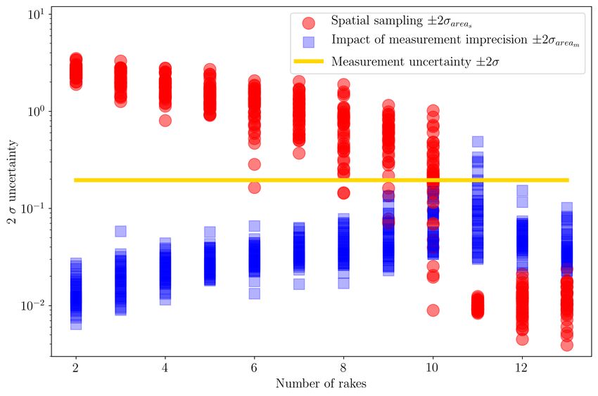
2 SESHADRI, DUNCAN, THORNE, PARKS, GIROLAMI
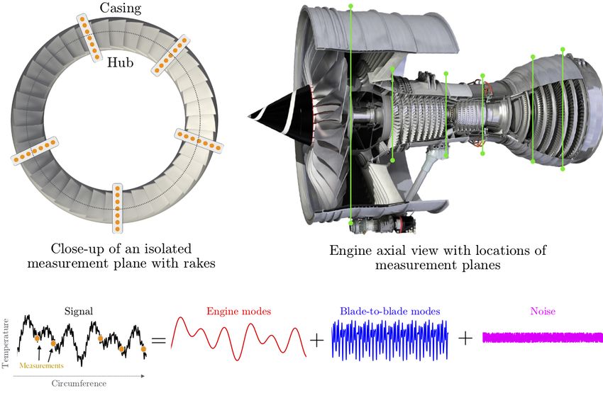
Figure 1. Close-up of an axial measurement plane in an engine. Each plane is fitted with circumferentially
scattered rakes with radially placed probes. The circumferential variation in temperature (or pressure) can be
broken down into various modes, as shown.
dial probes on each rake—are used to measure pressure and temperature values (see Figure 1).
These measurements are aggregated through area- or mass-averages of the circumferentially
and radially scattered measurements at a given axial plane.
When provided with only temperature or pressure measurements, area-based averages are
used. These are typically estimated by assigning each sensor a weight based on the sector
area it covers. This weight will depend on the total number of sensors and the radial and
circumferential spacing between them (see [43, 12]). This sector area-average is computed
by taking the weighted sum of each measurement and dividing it by the sum of the weights
themselves. In practice, this recipe offers accurate estimates if the spatial distribution of the
measured quantity is uniform throughout the measurement plane. For spatially non-uniform
flows, the validity of this approach hinges on the circumferential placement of the rakes and
the harmonic content of the signal. Should all the rakes be placed so as to capture the
trough of the wave forms, then the sector area-average will likely underestimate the true area-
average. A similar argument holds if the rakes are placed so as to capture only the peaks of
the circumferential pattern (see [40]). This motivates a new framework that addresses this
limiting stratagem.
A salient point to note here concerns the use and limitations [9] of a strictly computational
approach to estimate the pressures and temperatures. Today, aeroengine computational fluid
dynamics (CFD) flow-field approximations via Reynolds averaged Navier Stokes (RANS),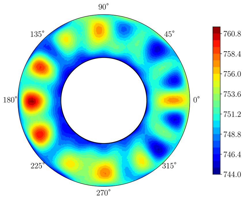
Bayesian Aeroengine Assessments                                                                  3

large eddy simulations (LES) [15] and, in some cases, via direct numerical simulations (DNS)
[49] are being increasingly adopted to gain insight into both component- and sub-system-level
design. These CFD solvers with varying fidelities of underpinning equations and corresponding
domain discretizations have found success—balancing simulation accuracy with simulation
cost—in understanding the flow-physics in the numerous sub-systems of an aeroengine (see
Figure 11 in [47]). However, in most cases, CFD-experimental validation is carried out using
scaled experimental rigs which typically isolate one sub-system or a few stages (rows of rotors
and stators) in an engine. Although there has been a tremendous body of work dedicated
to incorporating real-engine effects through aleatory [38, 39, 25] and epistemic uncertainty
quantification [11] studies, as a community, we are still far from being able to replicate the
aerothermal environment in engines: it is incredibly complex. For instance, the hub and casing
are never perfectly circular owing to variability in thermal and fatigue loads; engine structural
components introduce asymmetries into the flow that can propagate far downstream into the
machine, leading to flow-field distortions; and the pressure and temperature variations induced
by bleeds and leakage flows are not circumferentially uniform. The presence of these engine
modes make it challenging to use CFD in isolation to calculate aeroengine performance.
     Before we delve into the main ideas that underpin this paper, it will be helpful to under-
stand the experimental coverage versus accuracy trade-off. Sensor placement in an engine is
tedious: there are stringent space constraints on the number of sensors, the dimensions of each
sensor and its ancillary equipment, along with its axial, radial and tangential location in the
engine. However, engines offer the most accurate representation of the flow physics. Scaled
rigs, on the other hand, offer far greater flexibility in sensor number, type and placement, and
consequently yield greater measurement coverage, and while they are unable to capture the
engine modes–and thus are limited in their accuracy—they offer an incredibly rich repository
of information on the blade-to-blade modes. These modes include those associated with pe-
riodic viscous mixing (such as from blade tip vortices), overturning boundary layers between
two adjacent blades, and the periodic inviscid wakes [35, 24]. Although present in the engine
environment too, engines have insufficient measurement coverage to capture these blade-to-
blade modes. One can think of the spatial distribution of pressure or temperature as being a
superposition of such blade-to-blade modes (visible in rig experiments), engine modes (visible
in engine tests) and noise (see Figure 1). Succinctly stated, our best window on flow in an
aeroengine—and, in consequence, its composite temperatures and pressures—stems from real
engine measurements themselves. The challenge is that they are few and far between.
     Prior, publicly-available work has been rather limited and has largely focused on com-
puting uncertainty estimates of pressure and temperature based on the number of sensors,
rather than on an approximation of the flow-field itself [36]. Bonham et al. [2] state that, for
compressors, at least seven measurements are required in the radial direction, and at least five
measurements in the circumferential direction to resolve the flow. This is a heuristic, based
on the negligible change in isentropic efficiency if more measurements are taken. It should be
noted that this assessment is not based on a spatial model, but rather on experimental obser-
vations for a compressor with an inlet stagnation temperature of 300 Kelvin and a polytropic
efficiency of 85% at three different pressure ratios. In other words, it is difficult to generalise
this across all compressors.
     In [40, 37], the authors present a regularized linear least squares strategy for estimating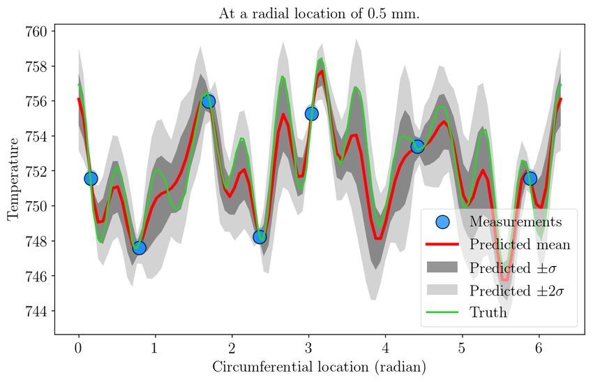
4                                              SESHADRI, DUNCAN, THORNE, PARKS, GIROLAMI

the spatial flow-field from a grid of measurements formed by radial and circumferentially
placed probes. Their data-driven model represents the spatial flow-field in the circumferential
direction via a Fourier series expansion, while capturing flow in the radial direction using a
high-degree polynomial. Although an improvement in the state of the art, their model does
have limitations. For instance, the placement of probes may lead to Runge’s phenomenon (see
Chapter 13 in [46]) in the radial direction, while the harmonic content is set by the Nyquist
condition (see Chapter 4 in [44]) in the circumferential direction. Another hindrance, one
not systemic to their work, but one mentioned in several texts (see 8.1.4.4.3 in [36] and in
[29]), is the definition of the uncertainty associated with insufficient spatial sampling and that
associated with the imprecision of each sensor. This decomposition of the overall uncertainty
is important as it informs aeroengine manufacturers whether they need more measurement
sensors or whether they need to improve the precision of existing sensors. In this paper, we
argue that an assessment of uncertainty is only possible with a priori knowledge of the spatial
flow field.
    Broadly, our scope and aim in this paper is to extract aerothermal insight from engine
data. We define our problem as follows. Given an array of engine sensor measurements at
an axial plane (see Figure 2), we wish to formulate computationally feasible and statistically
rigorous techniques to:
      • construct a spatial model to approximate the flow-field at an axial station given the
         inherent uncertainty in the measurements and certain physical assumptions (see sec-
         tion 2.2);
      • compute the area-average of the stagnation pressure and temperature based on this
         model (section 4.1);
      • ensure that the model can provide these performance measures while remaining robust
         to missing data (see Figure 2(b) and section 7.4).
      • distinguish between uncertainty in the spatial model (and its averages) induced by
         sensor imprecision, and insufficient spatial sampling (section 5);
      • quantify the dominant circumferential harmonics leveraging some notion of sparsity
         (section 3.2);
      • prescribe recipes for assessing sensor sensitivity (section 6.1) and optimal placement
         of sensors (section 6.2).
    To achieve these goals, we design a Gaussian random field model with a spatial covari-
ance function to capture the circumferential and radial flow characteristics. To the best of
the authors’ knowledge, this paper represents one of the first applications of Bayesian statis-
tical modelling to engine data with the aim of resolving the underlying flow-field based on
noisy observations. At a higher level, this paper aims to answer a fundamental question that
has confounded turbomachinery engineers and designers for decades: how do we rigorously
quantify and decompose the uncertainties in measurements? The answer to this question has
consequences upon the way uncertainties are dealt with in scaled rigs, engine and rig per-
formance analysis, system design, and prognosis in aeroengines, gas turbines, centrifugal and
axial pumps.

    2. Gaussian process aeroengine model. Gaussian processes (GPs) provide a powerful
framework for nonparametric regression, where the regression function is modelled as a ran-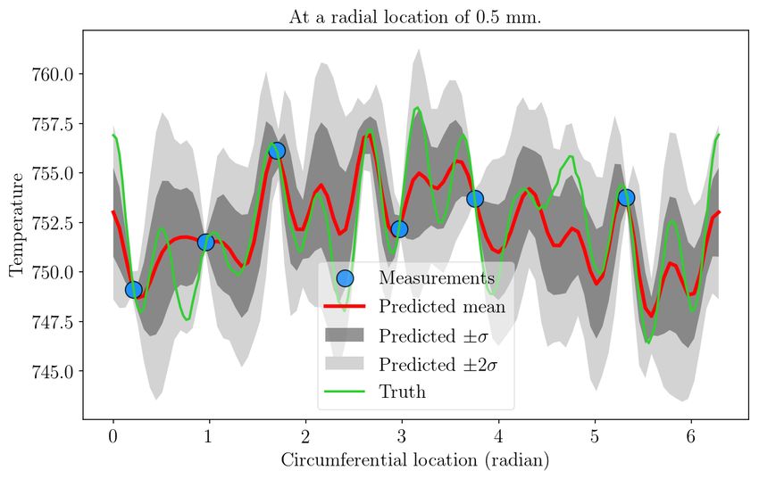
Bayesian Aeroengine Assessments                                                                         5

                       (a)                                                    (b)

    Figure 2. Engine temperature measurements (in Kelvin) obtained from circumferentially scattered rakes,
each with a finite number of radial probes. A standard measurement set in (a) and missing data in (b).

dom process, such that the distribution of the function evaluated at any finite set of points is
jointly Gaussian. GPs are characterised by a mean function and a two-point covariance func-
tion. GPs have been widely used to model spatial and temporal varying data since their first
application in modeling ore reserves in mining [22], leading to a method for spatial interpola-
tion known as kriging in the geostatistics community [8, 42]. The seminal work of Kennedy
and O’Hagan provides a mature Bayesian formulation which forms the underpinnings of the
approach adopted in this paper. Emulation methods based on GPs are now widespread and
find uses in numerous applications ranging from computer code calibration [16] and uncer-
tainty analysis [26] to sensitivity analysis [27]. Since then GP regression has enjoyed a rich
modern history within uncertainty quantification [20], with increasingly sophisticated exten-
sions beyond the classical formulation, including latent space models [7], multi-output models
[1] and GPs with incorporated dimension reduction [23, 41].
     In this section, we present a GP aeroengine spatial model—designed to emulate the steady-
state temperature and pressure distributions at a fixed axial plane. Given the complexity of
the flow, our aim is to capture the primary aerothermal features rather than resolve the flow-
field to minute detail. One can think of the primary aerothermal features as being the engine
modes in the circumferential direction. In what follows we detail our GP regression model;
our notation closely follows the GP exposition of Rogers and Girolami (see Chapter 8 in [31]).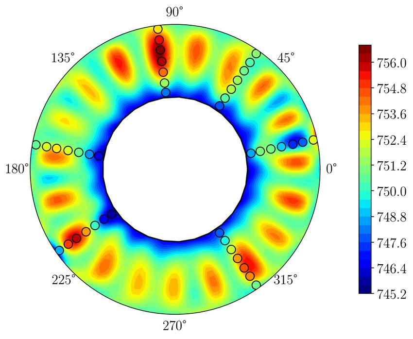
6 SESHADRI, DUNCAN, THORNE, PARKS, GIROLAMI
2.1. Preliminaries and data. Let us assume that we have sensor measurement location
and sensor reading pairs (xi , fi ) for i = 1, . . . , N and M locations at which we would like to
make reading predictions
∗ ∗
x1 f1 x1 f1
.. .. ∗ .. ∗ ..
(1) X = . f = . and X = . f = .
xN fN x∗M ∗
fM
2 N ×2 . Without loss
where the superscript (∗) denotes PN the latter. Here xi ∈ R , thus X ∈ R
in generality, we assume that i fi = 0, so that the components correspond to deviations
around the mean; physically, being either temperature or pressure measurements taken at
the locations in X. We assume that measurements in f are characterized by a symmetric
measurement covariance matrix Σ ∈ RN ×N with diagonal measurement variance terms σi2 for
i = 1, . . . , N . In practice, Σ, or at least an upper bound on Σ, can be determined from the
instrumentation device used and the correlations between measurement uncertainties, which
will be set by an array of factors such as the instrumentation wiring, batch calibration proce-
dure, data acquisition system and filtering methodologies. In the absence of measurements,
we assume that f is a Gaussian random field with a mean of 0 and has a two-point covariance
function k (·, ·). The joint distribution of (f , f ∗ ) satisfies
f KXX + Σ KXX ∗
(2) ∼ N 0, ,
f∗ KXX T
∗ KX ∗ X ∗
where the Gram matrices are given by
(3) [KXX ](i,j) = k(xi , xj ), [KXX ∗ ](i,l) = k(xi , x∗l ), and [KX ∗ X ∗ ](l,m) = k(x∗l , x∗m ),
for i, j = 1, . . . , N and l, m = 1, . . . , M . From (2), we can write the predictive posterior
distribution of f ∗ given f as
(4) P (f ∗ |f , X ∗ , X) = N (µ∗ , Ψ∗ ) ,
where the conditional mean is given by
−1
µ∗ = KXX
T
∗ (KXX + Σ) f
(5) T −1
= KXX ∗S f
with S = (KXX + Σ); the conditional covariance is
(6) Ψ∗ = KX ∗ X ∗ − KXX
T
∗S
−1
KXX ∗ .
2.2. Defining the covariance kernels. As our interest lies in applying Gaussian process
regression over an annulus, our inputs xi ∈ {(ri , θi ) : ri ∈ [0, 1] , θi ∈ [0, 2π)} can be parame-
terized as
r1 , θ1 r1 , θ1
(7) X = ... .. = r θ , and X ∗ = .. .. = r∗ θ ∗ .
. . .
rN , θN rM , θM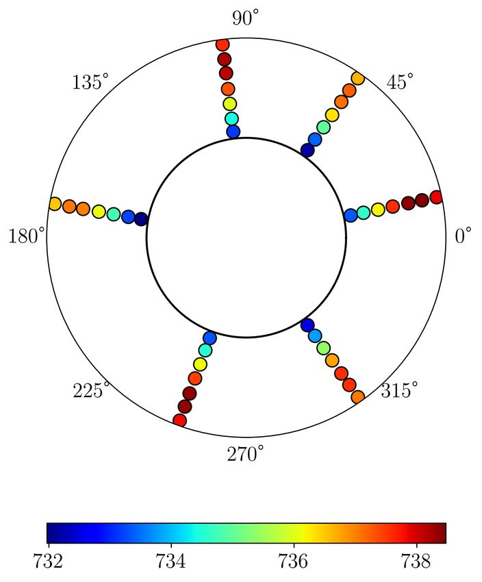
Bayesian Aeroengine Assessments 7
In most situations under consideration, we expect that
(8) X = {(ri , θj ) , ri ∈ r, θj ∈ θ} ,
where r is a set of L radial locations, and θ is a set of O circumferential locations, such that
N = L × O.
We define our spatial kernel to be a product of a Fourier kernel kf with a squared expo-
nential kernel ks
k x, x0 = k (r, θ) , r0 , θ 0
(9)
= kf r, r0 ks θ, θ 0 .
where the symbol indicates a Hadamard (element-wise) product1 .
We define the Fourier design matrix F ∈ R(2k+1)×N , the entries of which are given by
1 if i = 1,
sin ω i πθj /180 ◦ if i > 1 when i is even,
(10) Fij (θ) =
2
cos ω i−1 πθ /180◦
if i > 1 when i is odd,
j
2
where ω = (ω1 , . . . , ωk ) are the k frequencies used in the construction of the Fourier expansion
of the circumferential variation. Note that the number of columns in F depends on the size
of the inputs θ. We define the Fourier kernel
kf (θ, θ0 ) = F (θ)T ΛF θ0 ,
(11)
where
λ21
(12) Λ=
..
.
λ22k+1
is of size Λ ∈ R(2k+1)×(2k+1) and its diagonal elements are the hyperparameters that control
the variance of the Fourier modes; small values of λ2i will serve to limit the contribution of
the i-th mode. In the radial direction, the kernel has the form
0 2 1 0 T
0
(13) ks (r, r ) = σf exp − 2 r − r r−r
2l
where σf and l are the two hyperparameters to be determined.
We have assumed that our true measurements t ∈ RN are corrupted by a zero-mean
Gaussian noise, f = t+, with the noise being a function of sensor measurement imprecision.
As a result we observe f . This noise model, or likelihood, can be expressed as P (f |t, X) =
N (f , Σ), where we assume that Σ = σm 2 I, implying that the noise from the sensors has
constant variance and is independent. Using the Gaussian regression framework implies that
our model prior is Gaussian P (t|X) = N (0, KXX ). The central objective of our effort is
to determine the posterior P f |X, σm2 , σ 2 , l2 , λ2 , . . . , λ2
f 1 2k+1 . In the following section we will
prescribe priors on the hyperparameters to reflect a priori assumptions on the profiles.
1
For computational efficiency, the Kronecker product can also be used in cases where there are no missing
entries, i.e., sensor values can be obtained from a grid of measurements.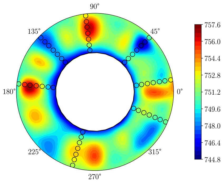
8                                                  SESHADRI, DUNCAN, THORNE, PARKS, GIROLAMI

               (a)                                 (b)                                  (c)

              (d)                                  (e)                                  (f)

   Figure 3. Three random samples from the Gaussian process prior with ω = [1, 3, 7, 12]; top row shows the
mean spatial field while the bottom row captures the standard deviation.

   3. Priors. In this section, we impose priors on the hyperparameters in (9). Priors for the
measurement noise and the squared exponential kernel are given by

                                            σm ∼ U [0, ] ,
(14)                                         α ∼ N + (0, 1) ,
                                              l ∼ N + (0, 1) ,

where  is an estimate of the standard deviation of the instrumentation measurement uncer-
tainty, N + represents a half-Gaussian distribution and U represents a uniform distribution.
Priors for the Fourier kernel are detailed below.

    3.1. Simple prior. There are likely to be instances where the precise harmonics ω are
known, although this is typically the exception and not the norm. In such cases, the Fourier
priors may be given by λi ∼ N + (0, 1), for i = 1, . . . , 2K + 1. In conjunction with the noise
and priors for the squared exponential kernel, this yields a total of 2K + 4 hyperparameters.
For completeness, we illustrate a few realizations from this Gaussian process prior in Figure
4 for a specific choice of ω = [1, 3, 7, 12], by selecting random values from the hyperparameter
priors. It is clear that the higher harmonics tend to dominate in (a) and (b), while the lower
harmonics are more prevalent in (c).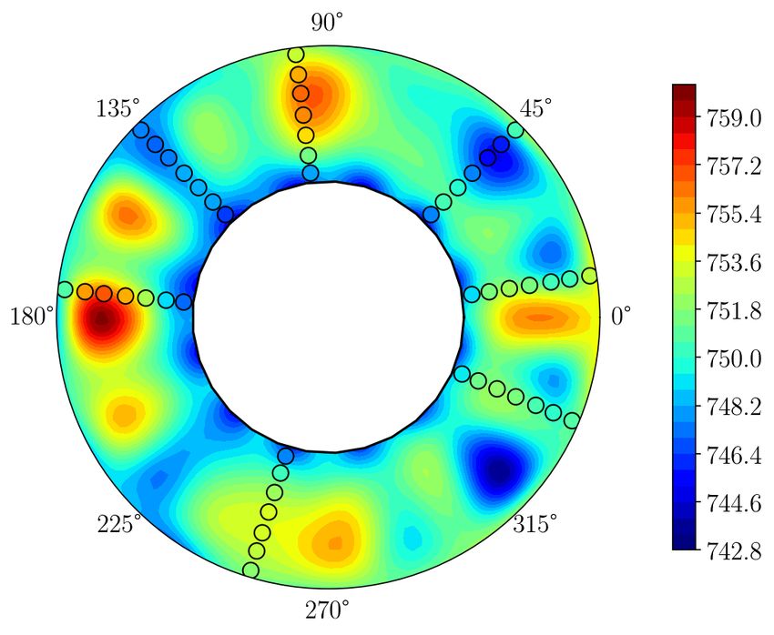
Bayesian Aeroengine Assessments                                                                9

    3.2. Sparsity promoting prior. In the absence of further physical knowledge, we constrain
the posterior by invoking an assumption of sparsity, i.e., the spatial measurements can be
adequately explained by a small subset of the possible harmonics. This is motivated by the
expectation of a sparse number of Fourier modes as contributing to the total variation. In
adopting this assumption, we expect to reduce the variance at the cost of a possible misfit.
Here, we engage the use of sparsity promoting priors, which mimic the shrinkage behaviour
of the least absolute shrinkage and selection operator (LASSO) [45, 4] in the fully Bayesian
context.
    A well-known shrinkage prior for regression models is the spike-and-slab prior [19], which
involves discrete binary variables indicating whether or not a particular frequency is employed
in the regression. While this choice of prior would result in a truly sparse regression model,
where Fourier modes are selected or de-selected discretely, sampling methods for such models
tend to demonstrate extremely poor mixing. This motivates the use of continuous shrinkage
priors, such as the horseshoe [5] and regularized horseshoe [30] prior. In both of these a global
scale parameter τ is introduced for promoting sparsity; large values of τ will lead to diffuse
priors and permit a small amount of shrinkage, while small values of τ will shrink all of the
hyperparameters towards zero. The regularized horseshoe is given by

                                       γ γs2

                             c ∼ IG      ,      ,
                                       2 2
(15)                        λ̃i ∼ C + (0, 1) ,
                                       cλ̃2i
                            λ2i =                ,   for i = 1, . . . , 2K + 1,
                                    c + τ 2 λ̃2i

where C + denotes a half-Cauchy distribution; IG denotes an inverse gamma distribution, and
where the constants
                                      βσm
(16)                       τ=            √ ,         γ = 30 and s = 1.0.
                                  (1 − β) N

The scale parameter c is set to have an inverse gamma distribution—characterized by a light
left tail and a heavy right tail—designed to prevent probability mass from aggregating close to
zero [30]. This parameter is used when a priori information on the scale of the hyperparameters
is not known; it addresses a known limitation in the horseshoe prior where hyperparameters
whose values exceed τ would not be regularized. Through its relationship with λ̃i , it offers
a numerical way to avoid shrinking the standard deviation of the Fourier modes that are far
from zero. Constants γ and s are used to adjust the mean and the variance of the inverse
gamma scale parameter c, while constant β controls the extent of sparsity; large values of β
imply that more harmonics will participate in the Fourier expansion, while smaller values of
β would offer a more parsimonious representation.
    4. Posterior inference. We generate approximate samples from the posterior distribution
jointly on f ∗ and the hyperparameters using Hamiltonian Monte Carlo (HMC) [10, 18]. In
this work, we specifically use the No-U-Turn (NUTS) sampler of Hoffman and Gelman [17],
which is a widely adopted extension of HMC. The main advantage of this approach is that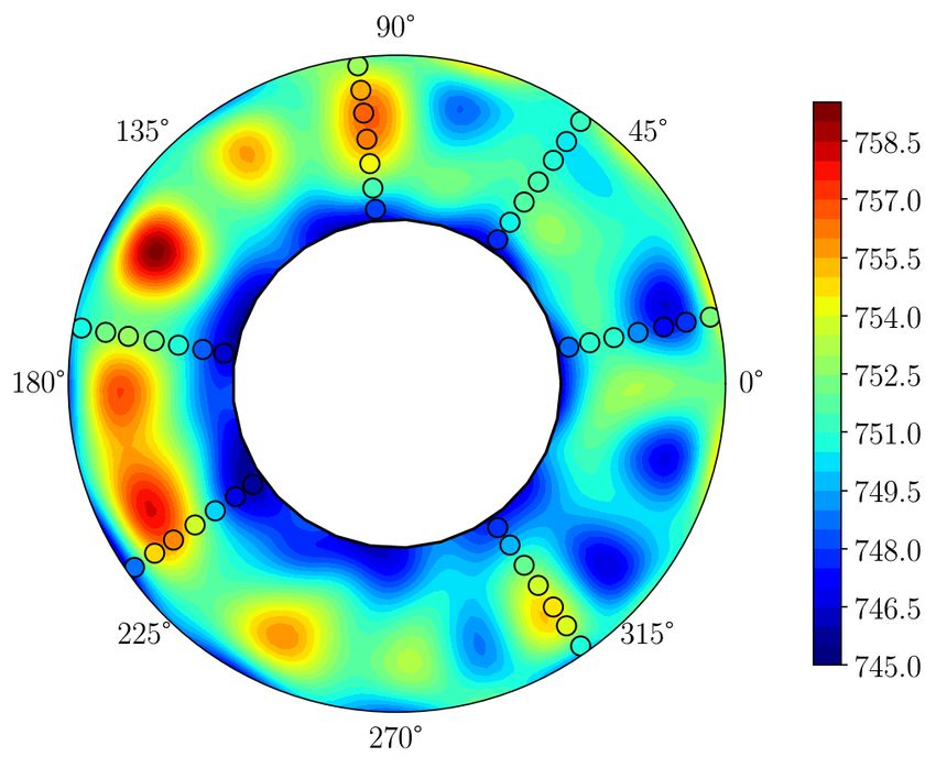
10                                                                     SESHADRI, DUNCAN, THORNE, PARKS, GIROLAMI

it mitigates the sensitivity of sampler performance on the HMC step size and the number of
leapfrog steps.

     4.1. Predictive posterior inference for the area average. The true area-weighted average
of a spatially varying temperature or pressure function y (x), where r ∈ [0, 1] and θ ∈ [0, 2π),
is given by
                                                                 Z   1 Z 2π
(17)                                         µarea [y] = ν                    y (r, θ) h (r) drdθ
                                                                 0     0

where
                          router − rinner
(18)               ν=       2        2
                                            and h (r) = r (router − rinner ) + rinner ,
                         π router − rinner

where rinner is the inner radius and router the outer radius. For notational simplicity, we
express (17) in its equivalent form
                                                                       Z
(19)                                              µarea [y] = ν            y (z) h (z) dz,

where z ∈ {(r, θ) : r ∈ [0, 1] , θ ∈ [0, 2π)} and the integral is taken over these bounds. We now
substitute y in (19) with our Gaussian process model f . Thus, the area-average of the spatial
field can be expressed in terms of the joint distribution
                                                        "                            R                      #!
                                                                   KXX + Σ        ν K (X, z) h (z) dz
(20)        R f (X)                          ∼N    0,                                                          .
           ν f (z) h (z) dz                                 ν K (z, X) h (z) dz ν 2
                                                             R                      RR
                                                                                       K (z, z) h2 (z) dzdz

Through this construction, we can define the area-average spatial quantity as a univariate
Gaussian distribution with mean
                                      Z
(21)                     µarea [f ] = ν K (z, X) h (z) dz S −1 f ,

where it should be clear that the posterior is obtained by averaging over the various hyper-
parameters. The variance is given by
                                        Z Z                         Z
             2
            σarea [f ]   =       ν   2
                                               K (z, z) h (z) dzdz − ν K (z, X) h (z) dz · S −1 ·
                                                             2

(22)                                                                 Z
                                                                     ν K (X, z) h (z) dz .

One point to note here is that although the integral of the harmonic terms is zero, the hyper-
parameters associated with those terms do not drop out and thus do contribute to the overall
variance.
Bayesian Aeroengine Assessments 11
5. Decomposition of uncertainty. To motivate this section, we consider the following
questions:
1. Can we ascertain whether the addition of instrumentation will alter the area-average
(and its uncertainty)?
2. How do we determine whether we require more sensors of the present variety, or higher
precision sensors at present measurement locations?
3. In the case of the former, can we determine where these additional sensors should be
placed?
As instrumentation costs in aeroengines is expensive, statistically justified reductions in instru-
mentation can lead to substantial savings per engine test. Thus, the answers to the questions
above are important. At the same time, greater accuracy in both the spatial pattern and its
area-average can offer improved aerothermal inference.
5.1. Spatial field covariance decomposition. To offer practical solutions to aid our in-
quiry, we utilize the law of total covariance which breaks down the total covariance into its
composite components cov [E (f ∗ |f , X)] and E (cov [f ∗ |f , X]). These are given by
−1
(23) cov [E (f ∗ |f , X)] = KXX
T
∗K
XX Ψf KXX KXX
∗
and
−1
(24) E (cov [f ∗ |f , X]) = KX ∗ X ∗ − KXX
T
∗K
XX KXX ,
∗
where
−1
−1
(25) Ψf = KXX + Σ−1 and µf = Σ−1 Ψf f ,
where once again we are marginalizing over the hyperparameters. We term the uncertainty
in (23) the impact of measurement imprecision, i.e., the contribution owing to measurement
imprecision. Increasing the precision of each sensor should abate this uncertainty. The re-
maining component of the covariance is given in (24), which we define as spatial sampling
uncertainty, i.e., the contribution owing to limited spatial sensor coverage (see [29]). Note
that this term does not have any measurement noise associated with it. Adding more sensors,
particularly in regions where this uncertainty is high, should diminish the contribution of this
uncertainty.
5.2. Decomposition of area average uncertainty. Extracting 1D metrics that split the
2
contribution of the total area-average variance into its composite spatial sampling σarea and
s
2
impact of measurement imprecision σaream is a direct corollary of the law of total covariance,
i.e.,
Z Z Z
2 2 2 −1
σarea s
= ν K (z, z) h (z) dzdz − ν K (z, X) h (z) dz · KXX
(26) Z
· ν K (X, z) h (z) dz
and
Z Z
2 −1 −1
(27) σarea m
= ν K (z, X) h (z) dz · KXX Ψf KXX · ν K (X, z) h (z) dz ,12 SESHADRI, DUNCAN, THORNE, PARKS, GIROLAMI
where ν and h were defined previously in (18). We remark here that whole-engine performance
analysis tools usually require an estimate of sampling and measurement uncertainty—with
the latter often being further decomposed into contributions from static calibration, the data
acquisition system and additional factors. Sampling uncertainty has been historically defined
by the sample variance (see 8.1.4.4.3 in [36]). We argue that our metric offers a more principled
and practical assessment.
Guidelines on whether engine manufacturers need to (i) add more instrumentation, or (ii)
increase the precision of existing measurement infrastructure can then follow, facilitating a
much-needed step-change from prior efforts [36, 29].
6. Sensitivity analysis and design of experiment. We begin this section with an as-
sumption, one that will become clear in the subsequent numerical examples section. We
assume that not all the measurements are equally important and that some—by virtue of
their location—make a greater contribution to the computed area-average. This naturally
leads to the questions of which sensor locations contribute the most information?
Here, we formulate a strategy for sensitivity analysis within the context of our model.
There is a tremendous body of literature on sensitivity analysis, both local and global [33].
Within a Gaussian process framework too, there exists papers on the use of (global) Sobol’
indices [32], and (the more local) Kullback-Leibler predictive relevances [28].
6.1. Sensitivity analysis of measurements. There are numerous local sensitivity metrics
that we can consider. To begin, imagine we perturb the temperature values at each of the
measured locations and want to determine which temperature value the area-average mean is
most sensitive to. This can be ascertained by computing
Z
∂µarea [f ]
(28) = ν R (z, X) h (z) dz S −1
∂fi
for each of the i-th measurements. Sensitivities with respect to the location Xij = (ri , θj ) of
existing instrumentation can also be computed for the mean area-average
Z
∂µarea [f ] ∂R (z, X) ∂µarea [f ]
(29) = ν h (z) dz S −1 where ∈ RN ×2
∂Xij ∂Xij ∂X
and its variance
2 2
Z
∂σarea [f ] ∂R (z, X) ∂σarea [f ]
(30) = −2 ν h (z) dz S −1 where ∈ RN ×2 .
∂Xij ∂Xij ∂X
6.2. Rake placement. There is a large repository of literature dedicated to experimental
design within a Bayesian context [6] and more specifically within Gaussian process regression
[21]. In [21] the authors discuss different objective functions including the interpretation of
classical A-, D-, E-optimal design in a Gaussian process context. Additionally, they study the
objectives of entropy and mutual information, advocating the use of the latter. Gorodetsky
and Marzouk [14] offer another objective, the integrated posterior variance, based on the
decomposition of the variance (see 3.1 in [14]); our objective for experimental design is very
similar to this.Bayesian Aeroengine Assessments 13
We are interested in determining which probe locations are best suited for minimizing the
area-average uncertainty, particularly when the number of circumferential rakes is less than
twice the number of harmonics. There are two reasons for this: (i) the addition of each rake
increases instrumentation costs; and (ii) more instrumentation in an engine will interfere with
the spatial flow pattern.
We define our problem as follows. Given O circumferential rakes at locations θ =
[θ1 , . . . , θO ]T , we wish to determine at which circumferential location an extra rake θ̂ could be
added such that σarea 2 is minimized. Assuming the locations of the radial probes on this new
rake are the same as the remaining rakes, we define
θ1
r1 ..
..
X̂ = r ⊗ 1O+1 , 1L ⊗ θ̂ , where r = . , θ̂ = . ,
(31)
θO
rL
θ̂
where 1O+1 and 1L correspond to a vectors of ones of lengths O + 1 and L respectively. Our
objective function can thus be stated as
2
(32) minimize σarea [f ]
θ̂
This optimization is non-convex and local minima can be obtained by using a gradient-based
optimizer, as gradients of this objective with respect to θ̂ can be analytically calculated. Note
that there are connections between the above and the fields of probabilistic integration and
probabilistic numerics (see [3] for further details).
7. Numerical results. To set the stage for an exposition of our formulations and algo-
rithms, we design the spatial temperature distribution shown in Figure 4. This field comprises
of five circumferentially varying harmonics ω = (1, 4, 7, 12, 14) that have different amplitudes
and phases going from the hub to the casing. A small zero-mean Gaussian noise with a stan-
dard deviation of 0.1 Kelvin is added to the spatial field. The computed area average mean
of the field is 750.94 Kelvin.
Throughout this section, we consider two distinct rake arrangements, where rakes are
placed at
θA = (12◦ , 55◦ , 97◦ , 170◦ , 215◦ , 305◦ ) ,
(33)
θB = (9◦ , 45◦ , 97◦ , 135◦ , 174◦ , 253◦ , 337◦ ) .
The former has six rakes while the latter has seven. Additionally, note that in θA , the
circumferential spacing between the forth and fifth rake is 45◦ and between the fifth and sixth
is 90◦ . This will undoubtedly have an impact on aliasing and may deter the sparsity promoting
prior from detecting the true spatial harmonics. We remark here that rake arrangements in
engines are driven by structural, logistical (access) and flexibility constraints, and thus, it is
not uncommon for them to be periodically positioned. As will be demonstrated, the rake
arrangements have an impact on the spatial random field and the area average, and thus we
will be comparing both rake arrangements (among others) throughout this section.14 SESHADRI, DUNCAN, THORNE, PARKS, GIROLAMI
(a)
Figure 4. Ground truth spatial distribution of temperature.
Table 1
Summary of sampling locations for the default test case.
Property name Symbol Value(s)
Rake arrangement A θA (12◦ , 55◦ , 97◦ , 170◦ , 215◦ , 305◦ )
Rake arrangement B θB (9◦ , 45◦ , 97◦ , 135◦ , 174◦ , 253◦ , 337◦ )
Probe locations (non-dimensional) r (0.07, 0.2, 0.35, 0.5, 0.66, 0.8, 0.95)
In what follows, we deploy some of the ideas presented in this paper to recover valuable
insight based on sparse measurements. Our codes use the open-source pymc3 [34] and the
numpy [48] python libraries.
7.1. Simple prior. We set our priors as per (14); harmonics to ω = (1, 4, 7, 12, 14), and
extract training data from the circumferential and radial locations provided in Table 1. Trace-
plots for the NUTS sampler for hyperparameters λ0 , λ1 , σf and l are shown in Figure 5 for rake
arrangement θA ; similar plots are obtained for rake arrangement θB . Note that these plots
exclude the first few burn-in samples and are the outcome of four parallel chains. The visible
stationarity in the these traces, along with their low auto correlation values give us confidenceBayesian Aeroengine Assessments 15
(a) (b)
(c) (d)
Figure 5. Traceplots for the MCMC chain for rake arrangement θA for some of the hyperparameters (a)
λ0 ; (b) λ1 ; (c) σf ; (d) l.
in the convergence of NUTS for this problem. The Gelman-Rubin statistic for all hyperpa-
rameters above was found to be 1.00; the Geweke z-scores were found to be well-within the
two standard deviation limit. Figure 6(a) plots the mean of the resulting spatial distribution
(ensemble averaged) for θA , while (b) plots its standard deviation. In comparing Figure 6(a)
with Figure 4, we note that in addition to adequately approximating the radial variation
(cooler hub and warmer casing), our methods are able to delineate the relatively hotter left
half-annulus and its three hot spots at 150◦ , 180◦ and 210◦ . This is especially surprising given
the fact that we have 5 spatial harmonics and only 6 and 7 rakes, and not the 11 needed as
per the Nyquist bound. A circumferential slice of these plots is shown in Figure 6(c) at a
radial height of 0.5 mm; a radial slice is shown in Figure 6(d) at a circumferential location of
0.21 radians. Here, we note that the true spatial variation (shown as a green line) lies within
the ±σ intervals in the circumferential direction, demonstrating that our approach is able to
provide sufficiently accurate uncertainty estimates in this case.
Similar results are reported in Figure 7 for θB . The position of the rakes has been inten-
tionally altered so as to capture the narrow cold spots at 135◦ and 225◦ . This has the effect16 SESHADRI, DUNCAN, THORNE, PARKS, GIROLAMI
(a) (b)
(c) (d)
Figure 6. Spatial distributions for (a) the mean and (b) the standard deviation, generated using an ensemble
average of the iterates in the MCMC chain, and a circumferential slice at (c) 0.5 mm and a radial slice at (d)
0.21 radians. Results shown for rake arrangement θA .
of reducing the overall spatial variance (see Figure 7(b)) by reducing the uncertainty along
the circumferential direction. More broadly, this result clearly articulates that even with fixed
harmonics, the placement of the rakes will have an impact on the predicted posterior.
7.2. Understanding uncertainty decompositions. For completeness we plot the decom-
position of the uncertainty for θA in Figure 8, where the contribution of impact of measurement
imprecision is, on average, an order of magnitude lower than that of spatial sampling. When
inspecting these plots one can state that reductions in the overall uncertainty can be obtained
by adding additional rakes at 215◦ and 300◦ (see Figure 8(b)). To assist in our understanding
of the spatial uncertainty decompositions above, we carry out a study varying the number of
rakes and their spatial locations. Figure 9 plots the two components of uncertainty for one,
two and three rakes, while Figure 10 plots them for nine, ten and eleven rakes. There are
several interesting observations to report.Bayesian Aeroengine Assessments 17
(a) (b)
(c) (d)
Figure 7. Spatial distributions for (a) the mean and (b) the standard deviation, generated using an ensemble
average of the iterates in the MCMC chain, and a circumferential slice at (c) 0.5 mm and a radial slice at (d)
0.21 radians. Results shown for rake arrangement θB .
First, the impact of measurement uncertainty deviates from the location of the sensor
with the accumulation of more rakes. For instance, in the case with one rake in Figure 9(a),
light blue and red contours can be found near each sensor measurement. However, as we
add more rakes, there seems to be a phase shift that is introduced to this pattern. This is
because the measurement uncertainty will not necessarily lie around the rakes themselves—
especially if knowledge about a sensors’ measurement can be obtained from other rakes—but
rather be in regions that are most sensitive to that particular sensor’s value. Furthermore,
in the case with an isolated rake, the impact of measurement imprecision locally will be
very close to the σ value assigned as the measurement noise. However, with the addition of
more instrumentation, the impact of measurement imprecision will increase, as observed in
Figure 9(g-i), before decreasing again once the spatial pattern is fully known (see Figure 10(g-
i)).18 SESHADRI, DUNCAN, THORNE, PARKS, GIROLAMI
(a) (b)
Figure 8. Decomposition of the standard deviations in the temperature: (a) impact of measurement impre-
cision, and (b) spatial sampling for θA .
Second, when the number of rakes is equal to eleven, the spatial sampling uncertainty
in the circumferential direction will not vary, and thus the only source of spatial sampling
uncertainty will be due to having only seven radial measurements. The former is due to the
fact that with five harmonics, we have eleven circumferential unknowns. This is clearly seen
in Figure 10(f). It should be noted that the position of the rakes can abate the uncertainties
observed. This raises a very important point concerning experimental design, and how within
a Bayesian framework, sampling uncertainty can be significantly reduced when the rakes are
accordingly positioned.
7.3. On area averaging. Area-average estimates are obtained by integrating the spatial
approximation (as per (20)) at each iteration of the previously presented MCMC chain, and
averaging over sample realisations. For the measurement configurations in Table 1, the area-
average computed is shown in Figure 11; also shown is the sector area-average, calculated by
weighting each measurement by each sensor’s area coverage, as discussed before. For rake
arrangement θA the Bayesian approach yields an area-average mean of 751.09 and a standard
deviation of 0.66 Kelvin; for θB we obtain 750.73 and a standard deviation of 0.45 Kelvin.
It will be useful to contrast this approach with the sector area approach. To do this, we
sample our true spatial distribution at forty different randomized circumferential locations for
different numbers of rakes, while maintaining the number of radial probes and their locations.
The circumferential locations are varied by randomly selecting rake positions between 0◦ and
355◦ inclusive, in increments of 5◦ . Figure 12(a) plots the resulting sector area-average. The
yellow line represents the true area-average and the shaded grey intervals around it reflect
the measurement noise. It is clear that the addition of rakes does not necessarily result in
any convergence of the area-average temperature. Furthermore, the reported area-average
is extremely sensitive to the placement of the rakes; in some cases a ±2 Kelvin variationBayesian Aeroengine Assessments 19
(a) (b) (c)
(d) (e) (f)
(g) (h) (i)
Figure 9. Decomposition of the standard deviations in the temperature for different number of rakes where
the top row shows the measurement locations, the middle row illustrates the spatial sampling uncertainty, and
the bottom row shows the impact of measurement imprecision. Results are shown for (a,d,g) one rake; (b,e,h)
two rakes; (c,f,i) three rakes.
is observed. In Figure 12(b) we plot the reported mean for each randomized trial using
our Bayesian framework. Not only is the scatter less, but, in fact, after 10 rakes we see that
reported area-averages lie not to far from the measurement noise. This makes a compelling case
for replacing the practice for computing area-averages in turbomachinery via sector weights
with a more rigorous Bayesian treatment.
We study the decomposition of the area-average variance in these randomized experiments
and plot their spatial sampling and impact of measurement imprecision components (see (26)20 SESHADRI, DUNCAN, THORNE, PARKS, GIROLAMI
(a) (b) (c)
(d) (e) (f)
(g) (h) (i)
Figure 10. Decomposition of the standard deviations in the temperature for different number of rakes where
the top row shows the measurement locations, the middle row illustrates the spatial sampling uncertainty, and
the bottom row shows the impact of measurement imprecision. Results are shown for (a,d,g) nine rakes; (b,e,h)
ten rakes; (c,f,i) eleven rakes.
and (27)) in Figure 13. As before, the measurement noise is demarcated as a solid yellow line.
There are interesting observations to make regarding these results.
First, the impact of measurement uncertainty increases with more instrumentation, till the
model is able to adequately capture all the Fourier harmonics (after eleven rakes); we made an
analogous finding when studying the spatial decomposition plots. This intuitively makes sense,
as the more instrumentation we add, the greater the impact of measurement uncertainty. It
is also worth noting that numerous rake arrangements can be found that curtail this sourceBayesian Aeroengine Assessments 21
(a) (b)
Figure 11. Area-average of the spatial distribution for the simple priors with reported mean and standard
deviations (a) Rake arrangement θA (751.09, 0.66); (b) Rake arrangement θB (750.73, 0.45).
(a) (b)
Figure 12. Convergence of (a) the sector-weighted area-average and (b) the Bayesian area-average (only
mean reported) for forty randomized arrangements of rake positions.
of uncertainty, many far below the threshold associated with the measurement noise.
Second, across the forty rake configurations tested, spatial sampling uncertainty contri-
butions were found to be very similar when using only two to three rakes. The variability in
spatial sampling uncertainty decreases significantly when the number of rakes is sufficient to
capture the circumferential harmonics. Thereafter, it is relatively constant, as observed by
the collapsing of the red circles in Figure 13.
7.4. On missing and anomalous measurements. Our Gaussian random field framework
permits easy detection and imputation of missing sensor data. Faulty sensors in an engine
can either give rise to anomalous readings or no readings at all. Within the engine test in-
strumentation infrastructure—which motivated our paper—anomalous readings can lie several
hundred degrees below or above the mode of all the measurements, while no readings typically
translate to obtaining an NaN output. Both of these eventualities can be easily detected and
the resulting sensor measurement location x = (r, θ) can be removed from the training data22 SESHADRI, DUNCAN, THORNE, PARKS, GIROLAMI
Figure 13. Decomposition of area-average spatial sampling and impact of measurement imprecision area-
average values for 40 randomized arrangements of rake positions.
for the Gaussian random field model. In the example we consider here, twenty-one out of the
total forty-nine measurements are set to be faulty; out of the seven measurements on each
rake in Figure 6 and Figure 7, three of them are removed.
In Figure 14 we plot the resulting spatial mean and area averages using NUTS. Even
with the faulty measurements, the model is able to recover some of the main temperature
characteristics from Figure 6 and Figure 7. Furthermore, the reported area-averages are fairly
robust to these missing measurements—in both mean and variance.
7.5. Sparsity promoting prior. Here, we set the priors as per (15); harmonics to ω =
(1, 2, . . . , 20), and extract training data from the circumferential and radial locations provided
in Table 1 for both θA and θB . Our goal in this section is to confirm whether our sparsity
promoting strategy—via the regularized horeshoe prior—can adequately identify that the true
spatial distribution was born from harmonics (1, 4, 7, 12, 14), when supplied with temperature
values on a limited number of rakes.
Figures 15 and 16 plot the convergence traces (a, b) and the prior samples for various two
dimensional marginal distributions in (c-e). It is clear from these plots (and others that were
viewed but are not shown) that the prior is able to ensure that MCMC iterates are either
close to zero or far away, and avoids having both across multiple Fourier hyperparameters. At
each iteration of the chain, the sampler is effectively subselecting a few harmonics that can
adequately explain the spatial variation gathered from the measurements. Geweke z-scores
[13] for the two different rake arrangements are shown in Figure 17, where for rake arrangement
A, barring two λ hyperparameters, all of them fall within the two standard deviation bound;
for rake arrangement B, all parameters fall well within. The Gelman-Rubin metric for all the
hyperparameters was found to be between 1.00 and 1.05.
The violin plots in Figure 18 capture the marginal distributions of the Fourier variance
hyperparameters; red distributions correspond to λ values associated with the cosine term ofBayesian Aeroengine Assessments 23
(a) (b)
(c) (d)
Figure 14. Spatial mean temperature fields and their corresponding area averages for Rake arrangements
(a, c) θA and (b, d) θB . In (c) and (d) the Standard readings correspond to the uncorrupted data cases in
Figure 6 and Figure 7 respectively.
the Fourier expansion, while the blue distributions are associated with the sine term. This
plot is useful in elucidating how the posterior distributions of all of the hyperparameters have
a strong spike centered around zero. Aside from this, a tabulated list of which frequencies
were chosen the most across the MCMC chains can be obtained, as shown in Tables 2 and
3. Figure 19 plots the ensemble mean and area averages across all the different frequency
choices enumerated by the chain for both rake arrangements. These mean spatial patterns,
while different from the ground truth (see Figure 4) are able to capture some of its features.
A few remarks regarding the results above are in order. First, the placement of the cir-
cumferential rakes has a significant impact on the estimated frequencies and spatial pattern.
In Figure 19(a) no instrumentation is placed near the cold spot at 135 degrees and the enu-
merated frequency breakdown for θA does not does have a (1, 4, 7, 12, 14) within the top ten
dominant harmonics. Our hypothesis for this observation is the inherent difficulty in detect-
ing the right frequency, given only six rakes, compounded with the fact that the latter three24 SESHADRI, DUNCAN, THORNE, PARKS, GIROLAMI
(a) (b)
(c) (d) (e)
Figure 15. MCMC output for the sparse prior model for θA : (a) and (b) plot the trace and posterior dis-
tributions for λ7 and λ24 respectively. Marginal distributions for the prior distribution on the Fourier variance
hyperparameters (c) λ1 vs λ5 ; (d) λ15 vs λ37 and (e) λ3 vs λ7 .
Table 2
Dominant top ten harmonics iterated upon for Rake arrangement θA .
Frequency selected Percentage of iterations
(2, 15, 17, 20) 4.65
(5, 7, 15, 17) 3.71
(10, 12, 17, 19) 2.81
(10, 17, 19, 20) 2.73
(17, 19, 20) 2.30
(2, 5, 15, 17) 1.82
(1, 4, 19, 20) 1.72
(4, 17, 19, 20) 1.53
(1, 5, 7, 15) 1.52
(8, 10, 11, 19) 1.49Bayesian Aeroengine Assessments 25
(a) (b)
(c) (d) (e)
Figure 16. MCMC output for the sparse prior model for θB : (a) and (b) plot the trace and posterior dis-
tributions for λ7 and λ24 respectively. Marginal distributions for the prior distribution on the Fourier variance
hyperparameters (c) λ1 vs λ5 ; (d) λ15 vs λ37 and (e) λ3 vs λ7 .
(a) (b)
Figure 17. Geweke z-scores for the sparse prior cases. For rake arrangements (a) θA and (b) θB .26 SESHADRI, DUNCAN, THORNE, PARKS, GIROLAMI
(a)
(b)
Figure 18. A violin plot showing the Fourier hyperparameter marginals. Red distributions correspond to
λ values associated with the cosine term, while blue distributions correspond to the sine term across the 20
harmonics. For rake arrangements (a) θA and (b) θB .
rakes are 45◦ and 90◦ apart, as mentioned earlier in this section. It could be argued that rake
arrangement in θB offers a more comparable spatial pattern with the ground truth; it is clear
that the harmonics selected (on average) are lower than in θA . Additionally, within the top
ten harmonics, the frequencies (1, 4, 7) appear at several instances, giving us confidence in the
predictive capabilities of the sparsity promoting prior. Unsurprisingly, in both cases, reported
area average values are fairly robust to the uncertainty in both spatial frequency and selected
hyperparameter values, which once again is because of the effect of integrating the Fourier
terms.
Conclusions. Understanding the spatial annular pattern born from engine measurements
provides valuable aerothermal insight. This paper represents a systematic and rigorous effort
to arrive at such a spatial pattern and its underlying uncertainty. Future work will focus on
techniques to leverage empirical data in conjunction with physics-based insight to determine
which frequencies to use for the circumferential harmonics.
Acknowledgments. The authors are grateful to Raúl Vázquez Dı́az and Duncan Simpson
(Rolls-Royce). This work was funded by Rolls-Royce plc; the authors are grateful to Rolls-
Royce for permission to publish this paper. PS, AD and MG would also like to acknowledge
the support of the Lloyd’s Register Foundation Data-Centric Engineering programme of theBayesian Aeroengine Assessments 27
(a) (b)
(c) (d)
Figure 19. Spatial mean temperature fields and their corresponding area averages for Rake arrangements
(a, c) θA and (b, d) θB for the sparse prior. In (c) and (d) the simple prior corresponds to the fixed harmonic
cases in Figure 11.
Table 3
Dominant top ten harmonics iterated upon for Rake arrangement θB .
Frequency selected Percentage of iterations
(1, 4, 9, 12, 14) 6.62
(1, 4, 7, 8, 19) 3.87
(1, 3, 7, 15, 20) 3.65
(1, 11, 12, 13, 15) 3.41
(1, 4, 7, 12, 14) 3.10
(1, 2, 3, 4, 18) 2.23
(1, 4, 7, 16, 18) 1.99
(1, 4, 9, 14, 20) 1.97
(1, 4, 7, 9, 16) 1.83
(1, 7, 10, 12, 18) 1.6028 SESHADRI, DUNCAN, THORNE, PARKS, GIROLAMI
Alan Turing Institute.
REFERENCES
[1] I. Bilionis and N. Zabaras, Multi-output local Gaussian process regression: Applications to uncertainty
quantification, Journal of Computational Physics, 231 (2012), pp. 5718–5746.
[2] C. Bonham, S. J. Thorpe, M. N. Erlund, and R. Stevenson, Combination probes for stagnation
pressure and temperature measurements in gas turbine engines, Measurement Science and Technology,
29 (2017), p. 015002.
[3] F.-X. Briol, C. J. Oates, M. Girolami, M. A. Osborne, D. Sejdinovic, et al., Probabilistic
integration: A role in statistical computation?, Statistical Science, 34 (2019), pp. 1–22.
[4] P. Bühlmann and S. Van De Geer, Statistics for High-Dimensional Data: Methods, Theory and
Applications, Springer Science & Business Media, 2011.
[5] C. M. Carvalho, N. G. Polson, and J. G. Scott, Handling sparsity via the horseshoe, in Artificial
Intelligence and Statistics, 2009, pp. 73–80.
[6] K. Chaloner and I. Verdinelli, Bayesian experimental design: A review, Statistical Science, (1995),
pp. 273–304.
[7] P. Chen, N. Zabaras, and I. Bilionis, Uncertainty propagation using infinite mixture of Gaussian
processes and variational Bayesian inference, Journal of Computational Physics, 284 (2015), pp. 291–
333.
[8] N. Cressie, Statistics for spatial data, John Wiley & Sons, 2015.
[9] J. D. Denton, Some limitations of turbomachinery CFD, in ASME Turbo Expo 2010: Power for Land,
Sea, and Air, American Society of Mechanical Engineers Digital Collection, 2010, pp. 735–745.
[10] S. Duane, A. D. Kennedy, B. J. Pendleton, and D. Roweth, Hybrid Monte Carlo, Physics Letters
B, 195 (1987), pp. 216–222.
[11] M. Emory, G. Iaccarino, and G. M. Laskowski, Uncertainty quantification in turbomachinery simu-
lations, in ASME Turbo Expo 2016: Turbomachinery Technical Conference and Exposition, American
Society of Mechanical Engineers Digital Collection, 2016.
[12] S. T. Francis and I. E. Morse, Measurement and Instrumentation in Engineering: Principles and
Basic Laboratory Experiments, vol. 67, CRC Press, Boca Raton, FL, 1989.
[13] J. Geweke, Evaluating the accuracy of sampling-based approaches to the calculation of posterior moments,
vol. 196, Federal Reserve Bank of Minneapolis, Research Department Minneapolis, MN, 1991.
[14] A. Gorodetsky and Y. Marzouk, Mercer kernels and integrated variance experimental design: Con-
nections between Gaussian process regression and polynomial approximation, SIAM/ASA Journal on
Uncertainty Quantification, 4 (2016), pp. 796–828.
[15] N. Gourdain, F. Sicot, F. Duchaine, and L. Gicquel, Large eddy simulation of flows in indus-
trial compressors: a path from 2015 to 2035, Philosophical Transactions of the Royal Society A:
Mathematical, Physical and Engineering Sciences, 372 (2014), p. 20130323.
[16] D. Higdon, M. Kennedy, J. C. Cavendish, J. A. Cafeo, and R. D. Ryne, Combining field data
and computer simulations for calibration and prediction, SIAM Journal on Scientific Computing, 26
(2004), pp. 448–466.
[17] M. D. Hoffman and A. Gelman, The No-U-Turn sampler: adaptively setting path lengths in Hamilto-
nian Monte Carlo, Journal of Machine Learning Research, 15 (2014), pp. 1593–1623.
[18] A. M. Horowitz, A generalized guided Monte Carlo algorithm, Physics Letters B, 268 (1991), pp. 247–
252.
[19] H. Ishwaran and J. S. Rao, Spike and slab variable selection: frequentist and Bayesian strategies, The
Annals of Statistics, 33 (2005), pp. 730–773.
[20] M. C. Kennedy and A. O’Hagan, Bayesian calibration of computer models, Journal of the Royal
Statistical Society: Series B (Statistical Methodology), 63 (2001), pp. 425–464.
[21] A. Krause, A. Singh, and C. Guestrin, Near-optimal sensor placements in gaussian processes: Theory,
efficient algorithms and empirical studies, Journal of Machine Learning Research, 9 (2008), pp. 235–
284.
[22] D. G. Krige, A statistical approach to some basic mine valuation problems on the witwatersrand, JournalYou can also read