Towards a new MFF New priorities and their impact on Italy - CEPS

Towards a new MFF
 New priorities and their impact on Italy
 Giovanni Barci and Daniel Gros
 With Jorge Núñes Ferrer

 Abstract
This paper analyses the outlook for regional funding under the next Multiannual Financial Framework
of the EU for which the Commission has proposed new criteria. The starting point is the so-called Berlin
formula, developed from a blend of national and regional indicators. In reality, the allocation for any
region depends not only on the state of the region, but also heavily on the income level of the member
state in which this region is located.
The modifications to the Berlin formula proposed by the Commission would accentuate the importance
of the national component, despite the fact that the EU cohesion policy is supposed to aim at lagging
regions, not countries.
Growth in Italy has been below the EU average for some time. This means that the poorer Italian regions
should be entitled to a higher amount of cohesion policy funding. However, the increase one could
expect on this count is limited given the modifications to Berlin formula proposed by the Commission.
The application of the new formula would lead to a somewhat lower allocation for Italy overall
(especially for the Mezzogiorno) for two reasons: i) Italy is still a relatively prosperous member state, ii)
There are caps to the increase of cohesion policy funding to which regions can be eligible even if their
relative income position has worsened a lot.
Italian Universities and research institutes benefit less from EU funding than one would expect given
the size of the Italian economy from competitive support for research and innovation programmes
under Horizon 2020. This underperformance is not due to political decisions as the research funding of
the EU is allocated strictly on scientific merit.
In the area of research and innovation there is as well a strong north-south divide within the country.
Creating high quality research institutions in the south might be a more promising way to use cohesion
policy funds than building roads or railways. It should receive more attention and funding from national
and EU policymakers.

Contents
EU budget over time: an overview ................................................................................................. 1
 Introduction ..........................................................................................................................................1
 The evolution of EU budget ..................................................................................................................2
 The case of Italy ....................................................................................................................................4
Cohesion policy ................................................................................................................................ 6
 The future of Cohesion: a modified status quo?...................................................................................8
 Differential situation and needs in the convergence regions ...............................................................9
 The ‘Berlin formula’ ............................................................................................................................10
 Allocation MFF 2021-2027 and scenarios ...........................................................................................16
 Theoretical allocation vs Actual payments .........................................................................................21
Research and Innovation .............................................................................................................. 23
Conclusions .................................................................................................................................... 25
References ..................................................................................................................................... 27
Appendix ........................................................................................................................................ 29

List of Boxes, Figures and Tables
BOX 1: BERLIN METHOD EXPLAINED – COMMISSION PROPOSAL .................................................................................................12
BOX 2: THE IMPACT OF BREXIT .............................................................................................................................................21

FIGURE 1: EU BUDGET OVER TIME .......................................................................................................................................... 3
FIGURE 2: EU BUDGET OVER TIME – SHARES ............................................................................................................................ 4
FIGURE 3: EU PAYMENTS TO ITALY .......................................................................................................................................... 5
FIGURE 4: EU PAYMENTS TO ITALY – SHARES ............................................................................................................................ 5
FIGURE 5: THE CONVERGENCE PROCESS ................................................................................................................................... 7
FIGURE 6: GDP PER CAPITA AT PPS AS % OF THE EU AVERAGE, VISEGRÁD 4 VS ‘OLD SOUTH’.......................................................... 8
FIGURE 7: SHARE OF EU COHESION FUNDING IN TOTAL PUBLIC SPENDING ON INFRASTRUCTURE ....................................................... 9
FIGURE 8: REGIONAL CATEGORISATION – SCENARIOS ...............................................................................................................13
FIGURE 9: MORE CRITERIA AND LESS WEIGHT ON REGIONAL GDP ..............................................................................................14
FIGURE 10: STRUCTURAL FUNDS PER CAPITA...........................................................................................................................17
FIGURE 11: MFFS ALLOCATION – SCENARIOS .........................................................................................................................18
FIGURE 12: THE IMPACT OF DIFFERENT CRITERIA FOR REGIONAL CATEGORISATION .......................................................................19
FIGURE 13: DISTRIBUTIONAL CONSEQUENCES OF THE PROPOSED FORMULA ................................................................................20
FIGURE 14: THE IMPACT OF BREXIT .......................................................................................................................................21
FIGURE 15: HORIZON 2020 IN EU REGIONS ..........................................................................................................................23
FIGURE 16: R&D PERFORMANCE OF ITALIAN REGIONS AND PROVINCES ......................................................................................24
FIGURE 17. HORIZON 2020 TOTAL FUNDING (% OF GDP), ITALIAN REGIONS .............................................................................24
FIGURE 18: ITALIAN R&D PERFORMANCE OVER TIME ..............................................................................................................25

TABLE 1: NUMBER OF REGIONS IN EACH BUCKET .....................................................................................................................11
TABLE 2: CAPS ...................................................................................................................................................................15
TABLE 3: SAFETY NETS .........................................................................................................................................................15
TABLE 4: BERLIN METHOD – CALCULATIONS VS REAL ALLOCATIONS ............................................................................................17
TABLE 5: ALLOCATION FOR ITALY (ERDF, ESF+) .....................................................................................................................19
TABLE 6: BERLIN FORMULA PARAMETERS VS ESTIMATED COEFFICIENTS .......................................................................................22
TABLE 7: DATA CLUSTERING BASED ON MULTIANNUAL BUDGET HEADINGS ..................................................................................29
TABLE 8: COHESION POLICY FUNDS ALLOCATION DETERMINANTS: EVOLUTION OVER TIME .............................................................30
TABLE 9: HISTORIC OF ALLOCATIONS AND SCENARIOS FOR THE FUTURE .......................................................................................31

EU budget over time: an overview
Introduction
The current Multiannual Financial Framework (MFF) will end in 2020. There is not a lot of time left to
make substantial amendments to the proposal of the European Commission for the next MFF. It will
have to be decided, at the latest, under the German Presidency in the second half of 2020 to avoid the
controversial option of entering the provisional twelfths whereby the last year’s budget is disbursed in
equal instalments month by month.
It is already apparent that these negotiations will be at least as difficult as the previous ones.
Representatives from the so-called ‘Hanseatic league’ of net contributors have already indicated that
they are not willing to increase their net contribution to the EU budget, which would be necessary to
plug the gap left by Brexit. The proposal published by the Finnish presidency in late 2019 represents one
example of this.
Moreover, there will be competition for cohesion spending between the new member states, whose
growth has propelled them above certain thresholds for cohesion funding, and those countries/regions
from the south of the euro area which have fallen behind. In addition, the negotiations in the Council
are moving in a direction that deviates substantially from the European Parliament’s position, which has
reached cross party agreement on the future of the EU budget and may refuse consent if the budget is
not more ambitious.
This paper will provide first a longer-term overview of the main elements of the EU budget. It then
presents in more detail the distribution of regional funds under the so-called Berlin formula and the way
changes to this key for the distribution of Structural Funds proposed by the Commission would affect
cohesion funding.
There are two ways to analyse the budget of the EU, which sometimes give a different picture because
of the complicated process leading to actual spending. One can look at the funds which are allocated,
in principle for 7 years; or one can look at the sums actually spent each year.
The starting point for the budget process of the EU is the MFF, which provides an indispensable legal
framework, mandated by the Treaty. In principle, it provides an overall cap to spending (usually
expressed as a percentage of EU GNI) for the next 7 years and indications of the overall spending by
broad categories. However, actual spending is then determined by the annual budgets, which
sometimes diverge substantially from the patterns laid down in the MFF, especially if circumstances
have changed in the meantime, for example, due to delays in the implementation of the new legislation
and thus delays in commitments, or when a crisis materialises that requires expenditure by the EU
budget. This has been the case during the last MFF, when emergencies led to a re-direction of unspent
funds for new needs, such as migration or transfers of future commitments to earlier years to reinforce
youth employment programmes.
The variability of actual spending, relative to the one foreseen in the MFF is particularly pronounced for
cohesion policy, i.e. the Structural Funds, the European Social Fund and Cohesion Fund. The reason for
this is that disbursement under those funds requires the presentation and then implementation of
detailed projects at the regional level. Planning, approval and then implementation take years.
Projects and disbursements from the EU budget then come in tranches. This implies that actual
Cohesion spending is rather variable and always extends beyond the end of the MFF. Under the so-
called N+2 or N+3 rule, funds can be disbursed up to two to three years after the formal end of the MFF,
which is actually an improvement of the situation in multiannual frameworks before the rule was
introduced, which offered no limit to the time for disbursements of committed amounts. Actual
cohesion policy disbursements (payment commitments) fluctuate strongly due to the patterns of
implementation, while annual commitment levels are rather linear.

 1

Historically, payments have increased from about €25 billion per annum in the early 2000s (i.e. just
before enlargement) to about a peak of close to €60 billion in 2012/13, but have since fallen back to
below €30 billion in 2017. Preliminary data for 2018 indicate that cohesion spending has increased to
about €55 billion as implementation of projects for the 2014-2020 period accelerated. These few figures
illustrate the variability mentioned above. For longer comparisons one should go beyond the annual
figures.
Of course, these absolute values need to be read taking into account that the EU has enlarged from 15
to (now) 28 members.
Another factor making it difficult to pinpoint how much the EU does for its weaker members and regions
is that support for cohesion from the EU budget can take many forms. Cohesion policy is composed of
a number of different funds, i.e. the Cohesion Fund (CF), the Structural Funds (SF), composed of the
European Regional Development Fund (ERDF) and the European Social Fund (ESF). These are today
clustered under one common regulation1 together with the European Fund for Agriculture and Rural
Development (EARDF) and the European Maritime and Fisheries Fund (EMFF) and form the European
Structural and Investment Funds (ESIF), thereby streamlining the policy and making it more coherent.
But in addition to ESIF funding, the Common Agricultural Policy and several centrally managed funds
can also intervene in those regions. Those comprise for example the Horizon 2020 policy or the use of
supported equity and debt instruments from the competitiveness policy or the European Fund for
Strategic Investments (EFSI) and channelled through national financial institutions or the EIB.
This report, however, focuses solely on the Structural Funds (ERDF and ESF), which represent the main
support instrument for regions lagging behind.

The evolution of EU budget
Figure 1 shows the evolution of the EU budget over the last 18 years and the projections for the coming
7 years. Values are expressed in 2018 prices in order to appreciate real variations.2 The solid lines
represent actual payments provided to member states via the EU budget, while dotted lines are
projections based on the proposal for the next programming period submitted by the Commission in
May 2018.3

1
 Regulation (EU) No 1303/2013 of the European Parliament and of the Council of 17 December 2013 laying down
common provisions on the European Regional Development Fund, the European Social Fund, the Cohesion Fund,
the European Agricultural Fund for Rural Development and the European Maritime and Fisheries Fund and laying
down general provisions on the European Regional Development Fund, the European Social Fund, the Cohesion
Fund and the European Maritime and Fisheries Fund and repealing Council Regulation (EC) No 1083/2006
2
 2% yearly inflation is assumed.
3
 Commission proposal, May 2018.

 2

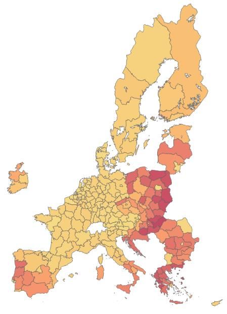
Figure 1: EU budget over time4

 EU budget over time
 MFF 2000-2006 MFF 2007-2013 MFF 2014-2020 MFF 2021-2027
 180000
 160000
 140000
 120000
 Euro, milions

 100000
 80000
 60000
 40000
 20000
 0
 2000
 2001
 2002
 2003
 2004
 2005
 2006
 2007
 2008
 2009
 2010
 2011
 2012
 2013
 2014
 2015
 2016
 2017
 2018
 2019
 2020
 2021
 2022
 2023
 2024
 2025
 2026
 2027
 CAP SF Other Tot

Source: European Commission and authors’ elaboration.

The budget of the EU has been under pressure since the Santer Commission scandal in 1999. At that
time the budget ceiling was fully utilised at 1.20% of GNI. The pressure to limit it to 1% was the result
of a steep fall in confidence both in the ability of the EU to manage resources properly, because of the
scandals surrounding the Commission itself and the high error rates and unaccounted sums in EU
support uncovered by the European Court of Auditors. Since then the EU budget has hovered around
an average of 1.1 % of GDP. Some increases were driven by enlargement, but the impact of enlargement
was moderate due to how the level of agricultural support was phased in for the new member states.
They benefit from relatively low subsidies as they were calculated using average yields for 2000-2003,
which was a period of weak production. Agriculture subsidies smoothly declined in the last programming
periods and a further drop is foreseen within the coming MFF. This is mainly due to the fact that
payments have been fixed in nominal terms, leading over time to a reduction in real terms. Structural
funds do not exhibit any clear trend and are expected to remain almost unchanged, although there have
been substantial fluctuations around the trend over time. Finally, “other” programmes have
experienced a sustained growth which is programmed to culminate by their overtaking CAP funds in the
coming MFF.
Figure 2 provides an overall view in terms of the shares of actual EU spending disbursed (not the sums
allocated under the MFF). It shows that the share of spending on agriculture has declined over recent
decades from about 50% to 40% of the total whereas spending on Research and Development has
increased from 4% to 8%. Cohesion spending has been more volatile. For the first ten years, i.e. between
2000 and 2010/11 it remained roughly constant at slightly above 30% of total EU spending. This was
followed by a peak towards the end of the last MFF (2013), when cohesion spending reached 40% of
the total, followed by a fall to below 30% in 2017. It remains to be seen whether cohesion spending will
pick up towards the end of the current MFF (i.e. in 2019/2020). The 2014-20 MFF had foreseen that
each year between 2014 and 2017 the appropriations for commitments should be higher for cohesion
spending than for agriculture, which would lead to increasing payments over time. The preliminary data
for 2018 might thus lead to a spike similar to 2012/3.

4
 See Appendix for clustering in CAP, SF, Other details.

 3

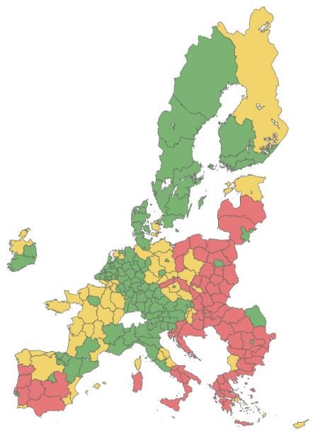
Figure 2: EU budget over time – shares

 EU budget over time - shares
 1 MFF 2000-2006 MFF 2007-2013 MFF 2014-2020 MFF 2021-2027

 0.9

 0.8

 0.7

 0.6

 0.5
 %

 0.4

 0.3

 0.2

 0.1

 0
 2001

 2006

 2011
 2000

 2002
 2003
 2004
 2005

 2007
 2008
 2009
 2010

 2012
 2013
 2014
 2015
 2016
 2017
 2018
 2019
 2020
 2021
 2022
 2023
 2024
 2025
 2026
 2027
 CAP_share SF_share Other_share

Source: European Commission and authors’ elaboration.

Overall, if one analyses actual spending as opposed to official plans, it appears that cohesion has de
facto maintained a roughly constant share of total EU spending (a bit below one third). The decline in
the share of agriculture has been matched by an increase in other spending. Research and Development
spending has roughly doubled its share, but it remains, at below 10%, much smaller than cohesion
spending.

The case of Italy
Figure 3 shows the evolution of the Italian situation vis-à-vis the EU budget. Net contributions from Italy
to the EU budget have increased over time (red solid line), mirroring a decline in EU payments (green
solid line). CAP transfers have followed a sustained and stable downward trend coherent with the EU-
whole picture. At a first sight, Structural Funds payments appear to have been declining slightly over the
last 18 years. However, it is important to stress that Figure 3 plots real payments while disregarding
allocations, which have been increasing in real terms.5 Moreover, despite the extremely volatile
trajectory followed EU disbursement related to Structural Funds, a clear cyclical component is
identifiable, which exhibits a substantial drop in the first years of each programming period followed by
a sharp recovery in the last part of the MFFs. It is interesting to notice that the expected decline lagged
two years in the MFF 14-20, reflecting the introduction of the n+2 rule. The share of “other”
programmes has increased over time. If these trends remain relatively undisturbed, a fairly even
distribution of EU funds should occur across the main categories of analysis during the next
programming period.

5
 See Appendix, Table 9.

 4

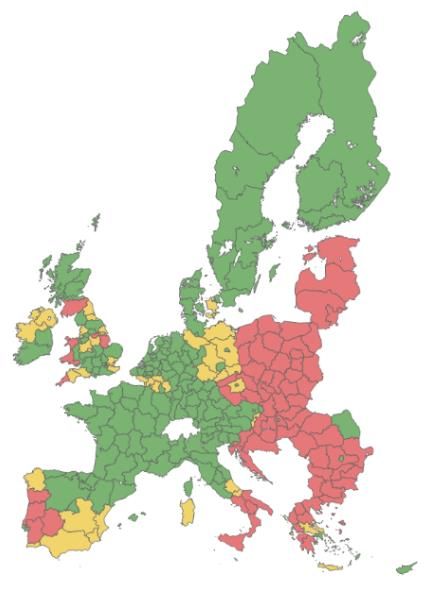
Figure 3: EU payments to Italy6

 EU payments to Italy
 20000 MFF 2000-2006 MFF 2007- MFF 2014-2020 MFF 2021-
 2013 2027
 15000

 10000
 Euro, millions

 5000

 0

 -5000

 -10000
 2001

 2017
 2000

 2002
 2003
 2004
 2005
 2006
 2007
 2008
 2009
 2010
 2011
 2012
 2013
 2014
 2015
 2016

 2018
 2019
 2020
 2021
 2022
 2023
 2024
 2025
 2026
 2027
 CAP SF Net payments Other Total payments

Source: European Commission and authors’ elaboration.

As highlighted in Figure 4, the relative evolution of EU budget components in Italy roughly retraces the
EU-wide trajectory. Although much smoother if compared to the EU average, there has been a drop in
the share of CAP transfers and the cohesion policy funds also fell while the share of “other” programmes
has increased.

Figure 4: EU payments to Italy – shares

 EU payments to Italy - shares
 1 MFF 2000-2006 MFF 2007- MFF 2014-2020 MFF 2021-
 2013 2027
 0.9
 0.8
 0.7
 0.6
 0.5
 %

 0.4
 0.3
 0.2
 0.1
 0
 2008

 2024
 2000
 2001
 2002
 2003
 2004
 2005
 2006
 2007

 2009
 2010
 2011
 2012
 2013
 2014
 2015
 2016
 2017
 2018
 2019
 2020
 2021
 2022
 2023

 2025
 2026
 2027

 CAP SF Other

Source: European Commission and authors’ elaboration.

6
 2018 prices, 2% yearly inflation.

 5

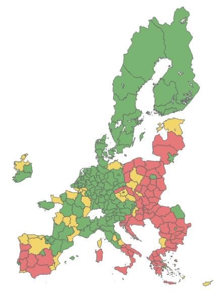
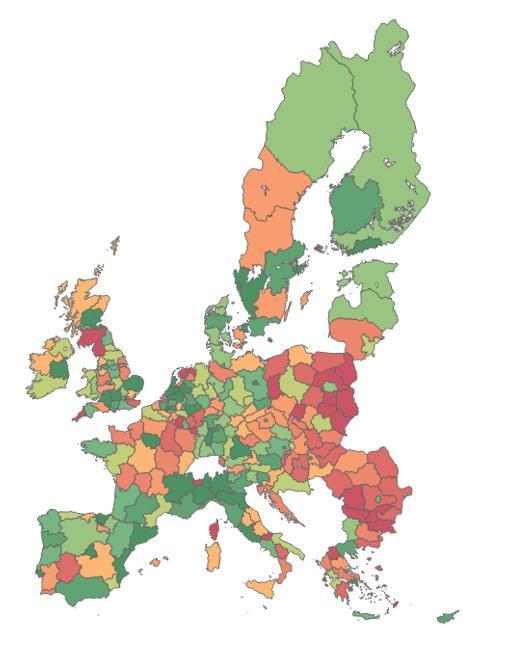
The rest of the paper will focus on the analysis of cohesion policy and especially on the R&D component
of “other” programmes.

Cohesion policy
Cohesion policy is the European Union’s strategy to promote and support the “overall harmonious
development” of its member states and regions. It, therefore, aims to foster a sustained convergence
process. This policy objective is fixed in the Treaty and is generally accepted as a basic pillar of the EU.
Cohesion policy is financed through the 3 main funds already presented, the ERDF, the ESF+ (both
representing what are called Structural Funds) and the CF. The ERDF and ESF+ are allocated on a regional
and project basis, while financing under the Cohesion Fund is transferred directly to member states.7
The main objective of the Structural Funds is to foster convergence among EU regions. Convergence in
the EU has improved, albeit with different degrees of success in different parts of Europe. Most regions
in the new member states show rapid convergence, whereas some in the south have been lagging
behind. Given the importance in terms of share of investment in the new member states of Structural
Funds, there are strong arguments to say they are playing an important role. It is more difficult to
separate the role of the EU funds on convergence where national public and social expenditure is much
bigger and the EU contribution less prominent. This is the case in Italian regions.
Looking at Figure 5, one finds a pattern of east-west convergence and north-south divergence. Regions
in eastern Europe followed a robust catch-up path. But the maps also show an impoverishment in most
southern regions, especially in Spain, Italy and Greece. What remains, for the time being, is a ‘bi-modal’
distribution: one finds a large number of regions between 75% and 90% and then above 105% of EU
average GDP, but relatively few below but close to 100%. Another problem that has emerged and been
exacerbated by the crisis, is an increased divergence also between economic centres within regions and
the periphery.
The Commission proposal represents an attempt to address the novel challenges raised by this uneven
progress in convergence.

7
 We do not consider other funds that could be deemed structural, such as EAGGF (European Agricultural Guidance
and Guarantee Fund) and FIFG (Financial Instruments for Fisheries Guidance), EMFF (European Maritime and
Fisheries Fund), EAFRD (European Agricultural fund for rural development), YEI (Youth Employment Initiative).

 6

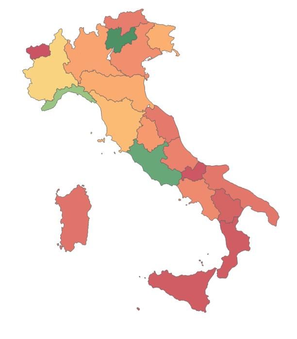
Figure 5: The convergence process8

Source: Eurostat and authors’ elaboration.

8
 Forecasts for 2024 are made assuming the economic growth rate of each region will be equal to the MS growth
rate (source: WEO updated October 2019, GDP capita PPP). In order to ensure comparability over time, we assume
no Brexit on these specific charts.

 7

The future of Cohesion: a modified status quo?
Fostering cohesion is a key aim of the European Union. A considerable part of the EU’s budget is thus
devoted to the cohesion policy whose purpose is to provide lagging regions and countries with the
means to catch up with the others. The new member states have benefitted from substantial allocations
of ESIF funds since they joined in 2004/7. This applies in particular to the ‘Visegrád Four’, which have
received between 2% and 3% of their GDP in cohesion policy funding, which has probably contributed
materially to the catch-up process.
In principle, EU cohesion support is destined mainly for “lagging regions”, i.e. those, with a GDP per
capita (at PPP) below 75% of the EU average. Transition regions, i.e. those with a GDP per capita
between 75% and 90% of the EU average and “more developed regions”, i.e. those with a GDP per
capita over 90% of the EU average can also benefit, but with lower amounts and for a more restricted
set of investment areas.
The relative success of the Visegrád countries is illustrated in Figure 6, which shows that jump of 20
percentage points (from 55% to 75% of the EU average) in the period 2000-2017. By contrast, the ‘old
south’ (Portugal, Spain and Greece) has fallen back, from a position much ahead of the V-4 (over 83%
of the EU average in 2000, to below 70% of the EU average and thus below the level now achieved by
the V-4).

Figure 6: GDP per capita at PPS as % of the EU average, Visegrád 4 vs ‘old south’.9

 Convergence, V-4 vs 'old south'
 100
 GDP per capita, PPS, % of EU average

 90 83
 80 75
 69
 70
 60 55
 50
 40
 30
 20
 10
 0
 V-4 Old South

 2000 2017

Source: European Commission, AMECO database.

While this reversal of fortunes is likely to create further tensions for the negotiations of the next MFF,
it also reveals that the use of the funds in the ‘old south’ or Mediterranean regions under convergence,
may have been sub-optimal to achieve more resilient and diversified economies. It also may indicate
national policy choices affecting the adaptability of the economy, e.g. Ireland not only grew quickly
beyond the EU average, but also recovered faster from the crisis, aspects that should open a serious
debate on structural aspects of development rather than the level or focus of EU funding.

9
 V-4 = average of PL, CZ, HU and SK; Old south = average of EL, ES and PT

 8

Differential situation and needs in the convergence regions
The development needs of regions in the Mediterranean and the new member states are different, and
the size of national budget for investment diverges. In the more advanced of the new member states,
the needs for investment in infrastructure is higher and investments in those areas will still show higher
returns. In some cases, the opportunity costs of building new infrastructure are very low, not requiring
the substitution of existing operational systems, e.g. there can be a technological leapfrog effect in
motion too. In the ‘old south’ a number of structural reform problems linger and investments in the
‘knowledge economy’ and new business models need to take a higher priority. In terms of value, the
impact of the funds is also very different due to the lower overall GDP and more limited size of national
budgets (as the convergence process is based on purchasing power parity calculations, a similar GDP
per capita for regional policy, measured in PPS, does not mean a similar nominal GDP).
Figure 7 below shows that in the new member states the EU has co-funded around one half of all public
spending on infrastructure. In Poland this ratio was even somewhat above 60 %, for the Czech Republic
still above 40 % (although one has to keep in mind that these figures also include co-financing by the
member state. While most new member states have benefitted from high amounts, they are not the
only ones, as the highest relative contribution to public sector infrastructure can be found in Portugal.
In Italy, by contrast, the ratio is only 12.8 %. This refers to the national average. If one looks at the poorer
regions in Italy, the corresponding figure is higher, in some case more than three times higher, but would
still remain below the values for the new member states because, as will be detailed below, poorer
Italian regions receive less regional funding as they are located in a member state with a still relatively
high average GDP per capita.

Figure 7: Share of EU cohesion funding in total public spending on infrastructure
 100
 90
 80
 70
 60
 50
%

 40
 30
 20
 10
 0
 Latvia

 Romania

 France

 Austria

 Denmark
 Croatia

 Hungary

 Greece

 Spain
 Italy

 Finland
 Poland

 Slovakia
 Bulgaria

 Slovenia
 Cyprus

 Netherlands
 Germany
 Ireland
 Portugal

 Lithuania

 Estonia
 Czech Republic

 Belgium

 Luxembourg
 Malta

 Sweden
 United Kingdom

Source: European Commission, https://cohesiondata.ec.europa.eu/Other/Share-of-Cohesion-Policy-per-Member-State-to-
publi/drqq-sbh7/data

The effectiveness of EU cohesion spending to foster growth in lagging regions was for a long time a hotly
contested issue, mostly for the spending in the EU-15.
Many regions in the old member states have by now received Structural Funds for a long time (25 years
and more), but have not converged. This is particularly the case in countries, which have experienced

 9

an overall crisis, like Greece, which, over the last decades has fallen back from a GDP per capita of over
85% of the EU average to about 67% today. Portugal has also fallen back, but by a smaller amount. Italy
is a special case in that it did not need to apply for funding from the financial stabilisation instruments
(EFSM or ESM), but its growth performance has, for almost a quarter of a century, been below that of
the rest of the euro area and of the whole EU.
By contrast, all of the new member states, have converged. At the present speed of convergence, new
member states (and all of the Visegrád 4) would enter the transitional regime (between 75% and 100%
of the EU average) during the next MFF based on their national averages. A key issue is whether this
uneven catch-up is due to differences in national policies or to circumstances beyond the control of
national governments.
The Commission has argued that “The potential of the EU budget can only be fully unleashed if the
economic, regulatory and administrative environment in the Member States is supportive. This is why,
under the current Multiannual Financial Framework, all Member States and beneficiaries are required
to show that the regulatory framework for financial management is robust, that the relevant EU
regulation is being implemented correctly, and that the necessary administrative and institutional
capacity exists to make EU funding a success.”10
Conditionality on ‘good governance’ might thus be an important element of the new MFF. In the present
MFF, for the first time ex ante conditionalities have been required. Countries whose regions are applying
for support in specific sectors, need to be in line with the EU regulations and directives for the sector.
The strategic requirements, monitoring and control have been updated and improved. The next MFF
will see more emphasis on good governance, not only on the rule of law, but on conditionality with
‘enabling conditions’,11 a further deepening of ex ante conditionalities, moving from formal compliance
to effective implementation.

The ‘Berlin formula’
Cohesion policy seems to have been successful in fostering convergence dynamics in the European
Union for most regions, particularly the poorest, but the policy and link to structural reforms needs to
be reinforced, given the uneven impact in different countries and the effect of the crisis. As presented
in the first chapter, about a third of the EU budget, corresponding to roughly €40-50 billion per year,
has been devoted to structural operations.
To understand the allocation of the funds, it is important to check the methodology. In a meeting held
in Berlin in 1999, the European Council set out a formula, now known as the ‘Berlin method’, to allocate
Structural Funds to regions and member states in a rigorous and transparent manner.12 The formula
was first adopted in the programming period 2000-2006 and has been modified ever since in each of
the subsequent periods. In May 2018, the European Commission submitted a proposal suggesting few
substantial adjustments to the Berlin method to allocate funds to regions within the coming multiannual
budget.

10
 Proposal for a Regulation of the European Parliament and of the Council on the protection of the Union's budget
in case of generalised deficiencies as regards the rule of law in the Member States, COM(2018) 324 final.
11
 Proposal for a Regulation of the European Parliament and of the Council laying down common provisions on the
European Regional Development Fund, the European Social Fund Plus, the Cohesion Fund, and the European
Maritime and Fisheries Fund, and financial rules for those and for the Asylum and Migration Fund, the Internal
Security Fund and the Border Management and Visa Instrument, COM(2018) 375 final
12
 “The new allocation method for the funds builds on the ‘Berlin formula’, adopted by the European Council in
1999” https://ec.europa.eu/commission/presscorner/detail/en/MEMO_18_3866

 10

Ultimately, the key drivers of cohesion funds allocation are regional income and socio-economic
regional indicators (see Box 1). Convergence being the primary purpose of cohesion policy, the Berlin
methodology ends up in allocating more resources to the worst performers.
The formula proposed by the Commission for the coming programming period distinguishes three
categories of regions (Table 1), each of whom are subject to different allocation criteria, for the
allocation of ERDF and ESF resources, which, combined, represent the great majority of cohesion
funding.13 The European regions are categorised as follows:
 1. Less developed regions (LDR) if their GDP per capita is less than 75% of EU-27 average,
 2. Transition regions (TR) if their GDP per capita is between 75%-100% of EU-27 average and
 3. More developed regions (MDR) if their GDP per capita is more than 100% of EU-27 average.
However, LDR and TR are treated differently, depending on the GNI (not GDP) of the member state (MS)
in which they are located, with three ‘buckets’:
 1. MS with a GNI per capita at PPS less than 82% of the EU-27 average,
 2. MS with a GNI per capita at PPS less than 99 % and more than 82% of the EU-27 average,
 3. MS with a GNI per capita at PPS above 99 % of the EU-27 average,
The fact that national wealth is taken into account when allocating cohesion funds means that, ceteris
paribus, a region in a richer member state will receive less resources than if it were to be part of a less
developed country. Eventually, the proposed classification would end up creating 7 categories.
Unfortunately, no justification is given for the precise numbers chosen to create these three buckets.

Table 1: Number of regions in each bucket14
 Regional classification (based on GDP pc at PPS of
 region (% of EU average) Total
 Below 75% Above 75% < 100% Above 100%
 MS classification Below 82% 52 8 (6) 66
 (based on GNI pc Above 82% < 99% 16 19 (20) 55
 at PPS of
 country, (% of Above 99% 3 34 (80) 117
 EU average)
 Total 71 61 106 238
Source: own calculations based on Eurostat.

While lagging regions tend to be part of poorer nations and richer regions tend to belong to wealthier
member states, only a third of transition regions are part of transition countries; the majority of
transition regions are located in wealthier member states.

13
 In the present analysis we do not consider EARDF nor EMFF. The Cohesion Fund is allocated at member state
level; hence it is not taken into account.
14
 Number of MDR are in parenthesis because their allocation is not affected by their respective national wealth.

 11

Box 1: Berlin method explained – Commission proposal
 Less Developed Regions (LDR):

 1. Prosperity gap  ∗ [ ∗ ( − )]
 
 2. Unemployment  ∗ [ − (
 
 ∗ )]
 ℎ 
 3. Youth unemployment  γ ∗ [ − (
 ℎ 
 ∗ ℎ )]

 4. Low education rate  δ ∗ [ 25−64 ∗ ( − )]

 Transition Regions (TR):

 1. Prosperity gap  ∗ [(0.6 ∗ ∗ − 54) + (72 − 0.6 ∗ ∗ ) ∗ % 

 A = 60% of the allocation a LDR
 A region whose GDP per capita is
0.6 * * ( -0.75* ) 75% of the EU average would
 receive
 B = average per capita aid that a
 MDR would receive
 B  linear interpolation between
 18
 A and B to calculate per capita
 allocation for transition regions,
 whose GDP is between 75% and
 75 GDP capita, % of EU27 100 100% of EU GDP
 average

 2. Unemployment, Youth unemployment, Low education rate bonuses apply in the same way as for the LDR

 More Developed Regions (MDR):

 Allocation of 18 EUR per total eligible population to be redistributed based on the relative regional share of**:

 1. Population (20%)  
 
 2. Unemployed (15%)  − (
 
 ∗ )

 3. Employed (20%)  25−64 ∗ ( − )
 4. Early leavers (15%)  18−34 ∗ ( − )
 5. Tertiary educated (20%)  30−34 ∗ ( − )
 6. GDP (7.5%)  ℎ ∗ − 
 7. Population density (2.5%)  3 < 12.5 ℎ 2

 Bonus that apply to all regions

 1. Greenhouse gas emissions  (national CO2 emissions2016 – 2030 emission target) ∗
 
 2. Net non-EU migration  400 ∗ [ ∗
 
 ]

 **Different weights applied in parenthesis; *** All allocation are per year

 12

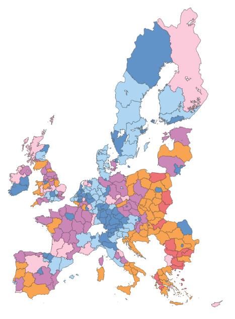
Retracing the backbone of the formulae that drove Structural Funds allocation in the current
programming period shows a number of substantial modifications in the methodology proposed by the
Commission for the next MFF. The Commission proposes to change the criteria through which eligible
regions are classified, the formulae to calculate regional allocations that apply to each of the above
described buckets, and sets boundaries that constrain the maximum and minimum transfers than a
region may receive.
Regarding the first set of modifications, the Commission proposes to increase the upper limit for a
region to be classified as ‘TR’, from 90% of average EU GDP per capita to 100%. As the Berlin method
sets different criteria to calculate allocations based in regional groups, the proposed change will have
clear implications for the regions that thus pass from being MDR to TR.15 Moreover, a reallocation of
regions in different groups has other effects as it modifies the group averages (e.g. unemployment rate,
education rate, employment rate, etc.). Given that the overall regional funds allocation depends on the
regions’ performance relative to group/EU averages, different averages lead to diverse allocations.
The maps in Figure 8 show the regional classification in the current programming period and present
two scenarios for the future MFF. The central panel pictures the classification in the current criteria
remaining unchanged, while the one on the right shows the regional classification under the proposed
formula. Regions are coloured red if LDR, yellow if TR and green if MDR. France and Germany seem to
be among the main beneficiaries of the revised methodology, as a relevant number of their regions
would happen to be classified as TR, instead of MDR.

Figure 8: Regional categorisation – scenarios

 MFF 2014-2020 MFF 2021-2027 MFF 2021-2027
 (Current Formula) (Proposed Formula)

Source: own calculations based on Eurostat.

The most prominent proposed modifications refer to the formulae that apply to each of the regional
categories and can be summarised as in Figure 9.

15
 See Box 1.

 13

Figure 9: More criteria and less weight on regional GDP

 Increased Complexity of indicators Evolution of relative wealth weights

 10 4.5
 4
 8
 Number of crteria

 3.5
 3
 6
 2.5

 %
 2
 4
 1.5
 2 1
 0.5
 0 0
 LDR TR MDR GNI < 82% GNI 82%-99% GNI > 99%

 MFF 07-13 MFF 14-20 MFF 21-27 MFF 07-13 MFF 14-20 MFF 21-27

Source: own calculations based on Eurostat.

The panel on the left indicates that complexity has increased over time as measured by the number and
the spectrum of socio-economic indicators taken into consideration.16 Furthermore, with the purpose
of tackling more horizontal challenges, which partially deviates from the primary objective of wealth
convergence – such as climate change and migration – the Commission proposed the introduction of
new criteria to be taken into account when calculating funds allocation
The panel on the right shows two key elements: the weight put on regional GDP has fallen over time
and the difference across different ‘classes’ of countries has widened considerably, at least if measured
in relative terms. For example, the first incarnation of the Berlin formula foresaw a weight of 4.1 on the
regional prosperity gap for regions in the poorest member states and a weight of 2.7 on the regional
prosperity gap in the richest MSs – a ratio of about 1:0.7. By contrast, the formula proposed by the
Commission foresees a weight of 2.7 on the regional prosperity gap in the poorest MSs and only 0.9 for
the richest. A ratio of 3:1. This implies that if one compares two regions with the same (low) GDP per
capita, but located in two different MSs, under the new MFF one would find that regions located in a
poor member state (GNI below 82% of EU average) would receive roughly three times as much as
another region, ceteris paribus, but located in a rich MS (GNI above the EU average). Under the original
Berlin formula, the region located in the poorer country would have received only about 50% more than
the one located in the rich country.
The ‘nationalisation’ of the regional allocations via the modulation of the weight on regional GDP
according to the prosperity of the MS had already started in 2007, but the proposals by the Commission
would represent another very important step.
The strengthening of the national effect is not offset by the other indicators mentioned above, which
are measured at the regional level, because GDP remains by far the most relevant indicator, driving
more than 80% of cohesion policy funds allocation.17 But, as pointed out, the decline on the weight of
prosperity gap has been less pronounced for poorer member states, implying that the ‘regional’ policy
of the EU has de facto become a policy aiming mainly at helping poorer member states. It is thus
becoming less regional and more national.

16
 See Appendix.
17
 Allocation of Cohesion policy funding to Member States for 2021-2027, ECA.

 14

Finally, the Commission proposes to modify the criteria to set the maximum and minimum allowed
regional allocations.
Within the present programming period, caps to structural finds allocation are used to avoid excessive
or insufficient concentration of resources. For the new Commission proposal, caps are set as follows: 18

Table 2: Caps
 CAP 2014-2020 Conditions CAP 2021-2027 (proposed) Conditions
 GDP caps
 2.35% of GDP Average real GDP growth 2.3% of GDP GNI per capita <
 2008-2010 higher than 1% 60% of EU average

 2.59% of GDP Average real GDP growth 1.85% of GDP GNI per capita
 2008-2010 lower than 1% 60%-65% of EU
 average
 1.55% of GDP GNI per capita >
 65% of EU average
 “Previous period” caps
 MS cannot receive more MS cannot receive more than -
 than 110% of its allocation 108% of its allocation for the
 for the 2007-2013 period 2014-2020 period
 MS cannot receive more than GNI per capita >
 its allocation for the 2014-2020 120% of EU
 period average
Source: Common Provisions Regulation 1303/2013 and Common Provisions Regulation proposal COM(2018) 321 final.

Furthermore, it has always been deemed politically inconvenient if EU funding were to change too
abruptly. This is why there were always some rules concerning changes in classification or when the
pure application of the rules were to lead to large changes because of rapid changes in the relative
income of regions or countries. This is also the case for the next MFF, where the Commission proposes
‘safety nets’ that are more generous than the ones in the current MFF as follows (Table 3).

Table 3: Safety nets
 Safety net 2014-2020 Safety net 2021-2027
 MS cannot receive less than 55% of its allocation for MS cannot receive less than 76% of its allocation for
 2007-2013 period 2014-2020 period
 TR cannot receive less than they would if they were TR cannot receive less than they would if they were MDR
 MDR
 Regions that lost their LDR status cannot receive less Regions that lost their LDR status cannot receive less
 than 60% of their annual allocation for the than 60% of their annual allocation for the Investment
 Investment for jobs and growth goal in the 2014- for jobs and growth goal in the 2014-2020 programming
 2020 programming period period
Source: Common Provisions Regulation 1303/2013 and Common Provisions Regulation proposal COM(2018) 321 final.

18
 See Appendix for a detailed description.

 15

Although the Commission proposes a reduction in the allowed negative variation amplitude relative to
the previous period allocation, there still remains a pronounced asymmetry between the positive and
negative variation bands. The maximum negative variation is proposed to be reduced from 45% to 24%
and the maximum positive variation from 10% to 8%. This is relevant because, in our calculations,
previous period caps seem to be much more binding than GDP caps.
That said, the amount allocated by the final inter-institutional agreements on the multiannual budget
are likely to diverge to some extent from the theoretical allocation suggested by the proposed changes
to the Berlin formula as the result of political negotiations, or the Council may require the formula to be
amended.

Allocation MFF 2021-2027 and scenarios
In order to analyse the implications of the proposed changes to the Berlin formula one needs to
calculate region by region the amount that would be allocated under the proposed new rules.
In the calculation we use the theoretically latest data available before the start of each programming
period, therefore 2006, 2013 and 2020. The 2020 data must of course be based on projections and are
calculated using growth rates forecasted by AMECO for GDP19 and GNI; for all other indicators forecasts
are calculated by applying the average growth rate experienced from 2014 to 2018 to 2018 data. For
the projections for the forthcoming MFF we use EU-27 averages to take Brexit into account.
We use these calculations for two purposes: first, we check whether for the two past MFFs (starting
2006 and 2013) our calculations based on the Berlin formula yield results that are close to the outcome.
This allows us to establish whether the Berlin formula was applied in reality (and whether our
calculations are materially correct). The calculations for the 2021-27 period allow us to forecast the
allocations per region Italy would receive under the proposed new formula.
On the first count, we find that the Berlin formula happened to be a very good predictor of the real
allocation of EU cohesion policy funds to member states. When regressing20 predictions calculated via
the Berlin method on the real allocations, one finds 96-98% of the variations in real allocation can be
explained by the Berlin method. The correlation between calculated and real values is extremely high
(0.98-0.99).
There are of course some outliers, but they concern only a few MS, while for the majority the difference
between predicted and actual allocations is limited, around 0-20%. These differences can be due to
many reasons. For example, changes can be agreed in the negotiation phase; discrepancies may also
result from the fact that growth projections at the start of the MFF turned out to be wrong and different
reference years or the absorption of funds may have been sub-optimal.
Notwithstanding the limitations mentioned, we consider the Berlin method a reliable tool to depict
different scenarios that may occur within the next multiannual programming period. Furthermore, the
discrepancy between predicted and real allocation for Italy is very limited (between 1% and 8%).

19
 National forecasted growth rates of GDP, measured in PPS, are assumed to apply indistinctly to all regions of
the nation.
20
 Simple cross-section OLS regression.

 16

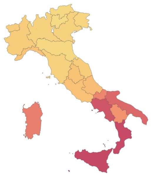
Table 4: Berlin method – calculations vs real allocations21
 MFF 2007-2013 MFF 2014-2020 MFF 2021-202722
 Data (average) - regional classification 2000-2002 2008-2010 2014-2016
 Data 2006 2013 2020
 Average prediction-real allocation discrepancy 29% 24% 15%
 (countries)
 Prediction-real allocation discrepancy (Total EU) 10% 2% 2%
 Italy prediction-real allocation discrepancy 8% 1% 4%
 Correlation prediction-real allocation 0.99 0.98 0.98
 R2 regression prediction-real allocation 0.98 0.96 0.96
 Coefficient regression prediction-real allocation 0.97 1.09 1.08
Source: Own calculations based on Commission data.

According to the prescriptions indicated in the proposal submitted by the Commission, we calculate the
theoretical regional cohesion policy funds allocation for the programming period 2021-2027.
Figure 10 below shows the relative distribution of cohesion funds per capita for the coming MFF. The
spectrum of colours is determined looking at the maximum and the minimum allocation and then
shaded accordingly. In the left panel minimum and maximum allocation refer to the whole EU, whereas
in the right panel they refer only to Italy.

Figure 10: Structural funds per capita
 EU-27 Italy

Source: Eurostat and authors’ elaboration based on the ‘Berlin method’.

The distribution of Structural Funds per head remains strongly concentrated in eastern countries. Lots
of resources are also directed to Greece, Portugal and the southern regions of Italy and Spain. The fact
that the shades of yellow are not easily distinguishable in richer regions means that the variations within
region groups (LDR, TR, MDR) is much less significant if compared with cross-group variation. This

21
 Calculations take into accounts the following Funds: ERDF, ESF, YEI, CF, ETC (EARDF, EMFF are not considered in
the analysis).
22
 Based on EU27 data (the proposed Berlin Formula assumes Brexit). The predicated-real allocation discrepancy
is relative to the Commission calculations, not real allocations. The discrepancy is most likely due to the fact that
we use 2020 forecasted data.

 17

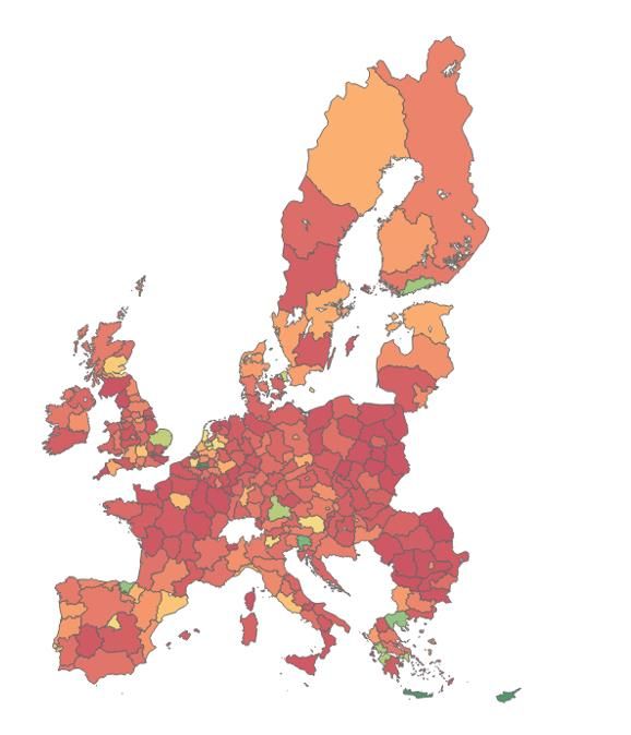
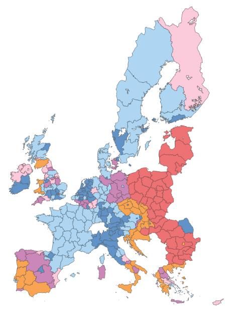
reflects the relevance of regional classification criteria and confirms the major implication that widening
the group eligible for transitional support proposed for the MFF 2021-2027 will have.
However, the maps in Figure 10 make it possible to appreciate how allocations may differ significantly
even within the same regional grouping, in per capita terms, mirroring the relative wealth of regions. If
looking at the real allocation the distribution is more homogeneous.
Looking to Italy, one notices a strong concentration on transfers to the southern regions. The majority
of resources are directed towards Sicilia, Calabria and Campania, which are expected to receive roughly
half of cohesion funds to Italy over the coming programming period, corresponding to about 18 billion.23
Looking at total allocation (not per capita), Campania, Sicilia and Puglia are among the main beneficiaries
in Europe, respectively at the 4, 5 and 12 position.
According to our calculations, Italy may expect to receive a similar amount of Structural Funds transfers
in the next MFF as in the current programming period. Notwithstanding, there may be relevant
distributional differences based on the actual allocation methodology that will be adopted. The maps in
Figure 11 show the difference, at the regional level, between actual allocations in MFF 2014-2020 and
the expected one for the coming MFF 2021-2027, both expressed in 2020 prices. We focus only on
significant changes, defined as more than 10% variations with respect to the current programming
period. Regions shaded in green will receive more funds, while red and grey mean respectively less
transfers and no sizeable variations (below +/- 10%). The first panel shows the allocation for Italian
regions if the current formula remains in place. For most regions the allocation will remain similar, 8
regions will receive more and only 3 will see their funds allocation reduced. The second panel shows the
allocation if the proposed formula is approved. All centre-north regions would receive more funds than
in the 2014-2020 programming period, while 5 southern regions would receive less. The minor
allocation to Sicilia, Calabria, Basilicata, Campania and Puglia reflects the proposed reduction in the
weight attached to GDP as driver of allocations. Panel 3 shows which regions would benefit and which
would be penalised if the proposed formula is applied, relative to the scenario in which the current
formula is not modified. Results highlight that the Mezzogiorno will be penalised.

Figure 11: MFFs allocation – scenarios24
 Scenario 1 – Current period formula Scenario 2 - Proposed formula Comparison

Source: Eurostat and authors’ elaboration based on the ‘Berlin method’.

23
 We consider only ERDF and ESF+, as regionally allocated funds
24
 In order to ensure comparability, allocation for the period 2014-2020 include only ERDF, ESF (CF and ECT are
included only to calculate caps and safety nets)

 18

Finally, in Figure 12 we propose an additional analysis in order to assess how variations within the new
proposed formula might affect funds distribution in Italy. The map plots which regions would benefit if
the current regional classification methodology (TR defined as those whose GDP per capita, measured
in PPS, is between 75%-90% of EU average, instead of 75%-100%, as proposed by the Commission) was
to be applied to the proposed formula. Although the allocation for most of the regions would be
unaltered, there would be major changes in few more developed regions (Emilia-Romagna, Trentino
and Friuli-Venezia Giulia). Marche clearly would be worse-off in this scenario, since it would be classified
as MDR and not TR. As aforementioned, different regional groups, results of different classification
criteria, produce different group averages, and, hence, diverse allocations.

Figure 12: The impact of different criteria for regional categorisation

Source: Eurostat and authors’ elaboration based on the ‘Berlin method’.

Our results can be summarised in the following tabular form:

Table 5: Allocation for Italy (ERDF, ESF+)25
 MFF 2014-2021 MFF 2021-2027

 Old formula €34 bn (€48bn)* €37 bn (€51 bn)*

 Proposed formula - €35 bn
* Figure in brackets indicate amount if caps did not apply.
Source: Own calculations based on Eurostat.

25
 See appendix for detailed regional allocation; allocations are expressed in 2020 prices (2% yearly inflation is
assumed); Previous period allocation caps take into account also YEI transfers (which the Commission proposed to
be included in the ESF (creating the ESF+) for the next programming period; Allocation for the EU27 would be 5%
lower if the proposed formula will substitute the old one (€270 billion instead of €285 billion).

 19

We account for the caps which stipulate that the increase from the previous period allocation cannot
be higher than 8% (in the proposed formula) and 10% (in the old formula). Numbers in parenthesis show
the allocations if caps did not apply. The caps on changes, which are tighter for increases than for falls
in allocation, thus play an important point for a country like Italy where the income of per capita of most
regions has declined considerably over the last 7 years.
Table 5 shows that the allocation for Italy in the MFF 2021-2027 under the new formula would be
€35 billion. This is not substantially different from the sum the country was allocated during the last
period. The new formula with its lower weight on GDP implies prima facie a substantial fall in the
allocation as the ‘old’ formula would have given Italy about €51 billion. But even under the old formula
the caps (limits on increases) would have prevented a substantial increase in the allocations. The
difference between the old formula and the one is thus relatively minor (€37 billion versus €35 billion).
However, the new formula would lead to a substantial reallocation within Italy: as shown in Figure 13,
the southern regions would receive less and the northern and central regions would receive more. The
reason for this is that the weight on GDP is lower, leading to a loss for the southern regions, but this is
made up by increases for the other regions on account of the unemployment and other indicators.

Figure 13: Distributional consequences of the proposed formula

 Scenario 1 – Current formula Scenario 2 – Proposed formula

 5% 2%
 6% 10%
 30% 25% 5%

 11%

 57%
 49%

The bottom line of our analysis is that Italy, according to the Commission proposal, will receive slightly
more funds relative to the current MFF (only about €1 billion spread over 7 years). Nonetheless, Italy
would be penalised by the new proposed methodology and by Brexit (see Box) in overall net
contributions. Southern Italian regions would receive, marginally, less than in the current programming
period.

 20