Particle Loss Calculator - a new software tool for the assessment of the performance of aerosol inlet systems
←
→
Page content transcription
If your browser does not render page correctly, please read the page content below
Atmos. Meas. Tech., 2, 479–494, 2009
www.atmos-meas-tech.net/2/479/2009/                                                                     Atmospheric
© Author(s) 2009. This work is distributed under                                                        Measurement
the Creative Commons Attribution 3.0 License.                                                            Techniques

Particle Loss Calculator – a new software tool for the assessment of
the performance of aerosol inlet systems
S.-L. von der Weiden1,2 , F. Drewnick1 , and S. Borrmann1,2
1 Particle    Chemistry Department, Max Planck Institute for Chemistry, Joh.-J.-Becher-Weg 27, 55128 Mainz, Germany
2 Institute   for Atmospheric Physics, Johannes Gutenberg University, Joh.-J.-Becher-Weg 21, 55128 Mainz, Germany
Received: 25 March 2009 – Published in Atmos. Meas. Tech. Discuss.: 22 April 2009
Revised: 7 August 2009 – Accepted: 19 August 2009 – Published: 3 September 2009

Abstract. Most aerosol measurements require an inlet sys-          (Brunekreef and Holgate, 2002). The great influence of
tem to transport aerosols from a select sampling location to a     aerosols over such a wide range of scales puts measure-
suitable measurement device through some length of tubing.         ments of integral, physical, and chemical aerosol properties
Such inlet systems must be optimized to minimize aerosol           such as size-distributions and size-resolved aerosol compo-
sampling artifacts and maximize sampling efficiency. In this       sition in high demand. Atmospheric aerosol particles cover
study we introduce a new multifunctional software tool (Par-       a size range of more than four orders of magnitude, from
ticle Loss Calculator, PLC) that can be used to quickly de-        freshly nucleated clusters having aerodynamic sizes of a few
termine aerosol sampling efficiency and particle transport         nanometers, to aged and cumulated particles and crustal dust
losses due to passage through arbitrary tubing systems. The        particles with sizes of several micrometers, to cloud droplets
software employs relevant empirical and theoretical relation-      with sizes on the order of millimeters. Aerosols are com-
ships found in established literature and accounts for the         prised of a large variety of materials having diverse prop-
most important sampling and transport effects that might           erties that change, along with overall aerosol concentration,
be encountered during deployment of typical, ground-based          over time (McMurry, 2000). These characteristics place high
ambient aerosol measurements through a constant-diameter           demands on measurement systems and instrumentation used
sampling probe. The software treats non-isoaxial and non-          to investigate them.
isokinetic aerosol sampling, aerosol diffusion and sedimen-           In recent years, both universities and research institutes
tation as well as turbulent inertial deposition and inertial de-   have been developing and improving aerosol measurement
position in bends and contractions of tubing. This software        instrumentation (e.g., Winklmayr et al., 1991; Gard et al.,
was validated through comparison with experimentally de-           1997; Weber et al., 2001; Orsini et al., 2003; Drewnick et al.,
termined particle losses for several tubing systems bent to        2005; Sagharfifar et al., 2009) to enable measurement of a va-
create various diffusion, sedimentation and inertial deposi-       riety of aerosol properties with high temporal resolution and
tion properties. As long as the tube geometries are not “too       accuracy. One important trend in aerosol science is the de-
extreme”, agreement is satisfactory. We discuss the conclu-        velopment of mobile laboratories which are able to measure
sions of these experiments, the limitations of the software        aerosol properties while underway. These mobile laborato-
and present three examples of the use of the Particle Loss         ries are typically equipped with instrumentation having high
Calculator in the field.                                           temporal resolutions and measure aerosol particle properties
                                                                   (and also gas loadings) in real time (Bukowiecki, 2002; Kit-
                                                                   telson et al., 2000; Kolb et al., 2004; Pirjola et al., 2004).
1   Introduction                                                      Because of this, high demands are placed on the sampling
                                                                   and inlet system that transports aerosols from outside of the
Aerosols affect the climate on a global scale (IPCC, 2007)         vehicle to each measurement device inside. Ideally, the inlet
as well as impact human and animal health on a local scale         system performs its function without changing aerosol char-
                                                                   acteristics, composition, concentration, or size distribution.
                        Correspondence to:                         In reality, sampling is non-ideal (non-isoaxial and/or non-
                        S.-L. von der Weiden                       isokinetic) and transport losses due to a number of mech-
                        (sl.vonderweiden@mpic.de)                  anisms (e.g. diffusion, sedimentation, inertial deposition)

Published by Copernicus Publications on behalf of the European Geosciences Union.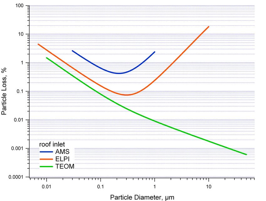
480                                                                        S.-L. von der Weiden et al.: Particle Loss Calculator

are often not negligible. These effects can cause signifi-         a bend, inertial deposition in a contraction, inertial deposition
cant changes in the aerosol properties prior to measurement        in an enlargement, electrostatic deposition, thermophoresis,
giving rise to unquantifiable uncertainties in spite of the        diffusiophoresis, interception and coagulation (Hinds, 1998;
fact that carefully calibrated measurement instrumentation         Willeke and Baron, 2005) and are described using the “trans-
is used. For instance, operational loss mechanisms during          port efficiency” (Sect. 2.3). Both sampling and transport ef-
sampling and transport depend on particle size. Small par-         ficiency are combined to yield an “overall efficiency” for the
ticles with an aerodynamic size below about 100 nm and             system (Sect. 2.1).
large particles with a size above about 0.5 µm are particu-           In the course of writing the Particle Loss Calculator, it
larly affected. When not accounted for, such non-uniform           was necessary to select formulas best suited to the program
particle losses can alter size-distribution measurements mak-      from a large variety available in the literature. In order to
ing a bimodal size distribution appear monomodal. Such             do so, all available formulas were collated and grouped ac-
discrimination also affects chemical composition measure-          cording to the quantity calculated. Equations for calculat-
ments since the substances comprising the particles are not        ing like quantities were compared with one another. Where
equally distributed with respect to particle size (Appel et al.,   different formulas resulted in different results, the equation
1988; Huebert et al., 1990; McMurry, 2000). To avoid er-           delivering the mean result was chosen and those giving ex-
roneous measurement results, new inlet systems should be           treme results omitted. Another criterion for the applicability
optimized prior to construction and properties of existing in-     of a formula is its range of validity. A wide range of valid-
let systems should be characterized to enable correction of        ity of the implemented relationships is preferable in order to
measurements.                                                      cover the maximum range of particle sizes and conditions in
   Recently, the Max Planck Institute for Chemistry in Mainz       arbitrary tubing systems. Finally, if there were two formulas
developed a mobile laboratory (“MoLa”) for flexible and            with similar results and application ranges, we implemented
mobile measurements of aerosol and gas concentration and           the simpler of the two in order to reduce the probability of
composition. As part of this development, the software Par-        programming errors and to minimize computing needs.
ticle Loss Calculator (PLC) was conceived as an efficient,            Almost all relevant particle loss mechanisms are described
flexible method for calculating particle losses due to sam-        well in the literature and implemented in the software. Only
pling to aid in inlet design for MoLa. The current ver-            the particle loss due to developing eddies in an enlargement
sion of the Particle Loss Calculator can be downloaded on          was omitted due to unsatisfactory publications and irrepro-
http://www.mpch-mainz.mpg.de/∼drewnick/PLC. The PLC                ducible calculations. Other loss mechanisms are neglected in
is written in the scientific programming environment IGOR          the software because their effects are several orders of mag-
Pro, which is also necessary to run the software. A free           nitude smaller than all other contributing terms under normal
IGOR trial version is available on www.wavemetrics.com.            sampling conditions (see Sect. 2.3.7). Based on these con-
   In Sect. 2, relevant aerosol loss mechanisms treated by the     siderations, the following sampling and particle loss mecha-
Particle Loss Calculator are described. The basis for se-          nisms are included in Particle Loss Calculator:
lection and use of the equations implemented for each loss
calculation is described in Sect. 3. In Sect. 4, comparison          – Non-isoaxial sampling (Sect. 2.2)
between validation experiments and calculations performed            – Non-isokinetic sampling (Sect. 2.2)
using the Particle Loss Calculator are discussed while three
sample applications of this calculator are described in Sect. 5.     – Diffusion (Sect. 2.3.1)

                                                                     – Sedimentation (Sect. 2.3.2)
2   Particle loss mechanisms
                                                                     – Turbulent inertial deposition (Sect. 2.3.3)
An aerosol sampling system generally consists of a sam-
                                                                     – Inertial deposition in a bend (Sect. 2.3.4)
pling probe and transport lines and, depending on aerody-
namic particle size, a variety of particle loss mechanisms           – Inertial deposition in a contraction (Sect. 2.3.5)
could be operative in any given system (e.g., Levin, 1957;
Davies, 1966; Fuchs, 1975; Vincent, 1989; Willeke and              The formulas implemented in the PLC only cover sampling
Baron, 2005). In the sampling probe, non-representative            effects through constant-diameter sampling probes. This
sampling comes from non-isoaxial and non-isokinetic condi-         software cannot be applied to other types of inlet geometries
tions related to movement of the air entering the probe. Here,     such as shrouded or diffusion inlets.
such losses due to extraction of aerosol particles from am-           The equations in the following description were ob-
bient air into the sampling system are described using the         tained either empirically through experimentation or de-
“sampling efficiency” (Sect. 2.3). The main particle loss          rived theoretically. Regardless of origin, each equation
mechanisms operative during transport are sedimentation,           is only applicable for a limited range of physical con-
diffusion, turbulent inertial deposition, inertial deposition in   ditions whose details can be found under the respective

Atmos. Meas. Tech., 2, 479–494, 2009                                                     www.atmos-meas-tech.net/2/479/2009/
S.-L. von der Weiden et al.: Particle Loss Calculator                                                                                      481

subsection for that equation and are also listed in Sup-               to inertia ηtrans,inert , respectively as a function of the aerody-
plement 1 (see http://www.atmos-meas-tech.net/2/479/2009/              namic particle diameter da (Willeke and Baron, 2005):
amt-2-479-2009-supplement.zip). An exceeding of the
range of validity in the calculation will be marked in the out-        ηsampling (da ) = ηasp (da ) ηtrans,grav (da ) ηtrans,inert (da )    (3)
put graph.                                                                In ideal situations the sampling is isoaxial and isokinetic.
   If no declaration is given for the unit of a quantity, SI-          Isoaxial means that the sampling probe faces straight into the
units are used. A complete list of the parameters as well              surrounding air motion (wind direction) with no inclination
as two figures showing all angles used in the relation-                (in general assumed as horizontal). The aspiration angle, θS ,
ships can be found in Supplement 1. The equations imple-               is then 0◦ . During non-isoaxial sampling, large particles can-
mented in the Particle Loss Calculator for particle trans-             not follow the curved streamlines leading into the sampling
port represent only a small selection of what is available             probe and, as a consequence, miss it (see Fig. 1).
in the literature. In Sect. 3, the criteria upon which equa-              Isokinetic sampling is related to the velocity ratio R re-
tions were selected are described. For reference, a com-               lating the local wind speed U0 to the flow velocity in the
plete list of the consulted publications can be found in Sup-          sampling probe U (Willeke and Baron, 2005):
plement 2 (see http://www.atmos-meas-tech.net/2/479/2009/
amt-2-479-2009-supplement.zip).                                                U0
                                                                       R=                                                                   (4)
                                                                               U
2.1   Overall efficiency ηinlet
                                                                       If the surrounding air velocity is higher than the flow veloc-
In general, the efficiency of a tube is defined as the ratio of        ity in the probe (R>1, U0 >U ), sampling is said to be sub-
the number concentration of particles behind the tube and the          isokinetic while the opposite (R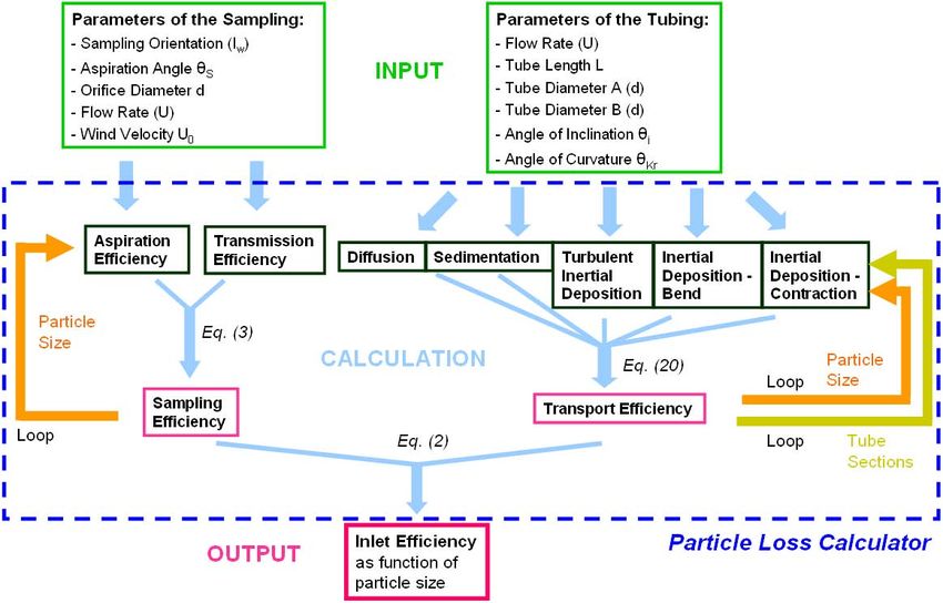
482                                                                             S.-L. von der Weiden et al.: Particle Loss Calculator

Fig. 1. Mechanisms occurring during aerosol sampling and transport in a sampling probe and a transport tube.

following relationship for the aspiration efficiency in mov-             For aspiration angles from 61◦ to 90◦ Hangal and Willeke
ing air under isoaxial sampling conditions based on a com-             (1990a) give:
bination of theoretical considerations and experimental data                             U0                      √
obtained by flash illumination photography:                            ηasp (da ) = 1 + (    cos(θS ) − 1)(3 Stk U0 /U )            (7)
                                                                                          U
                     U0              1                                 for 0.02≤Stk≤0.2, 0.5≤U0 /U ≤2.
ηasp (da ) = 1 + (      − 1)(1 −           )                  (5)
                     U           1 + k Stk                                If sampling in calm air, gravitational effects are no longer
                                                                       negligible and the terminal settling velocity Vts of the aerosol
where Stk=(da2 ρp CC U0 )/(18µd) is the Stokes Number of
                                                                       particles becomes important. The terminal settling velocity
the sampling probe (Willeke and Baron, 2005), ρp is the par-
                                                                       is defined in the Stokes Regime (Particle Reynolds Number
ticle density, CC =1+Kn(1.142+0.558 exp(−0.999/Kn)) is
                                                                       Rep 0◦ to 60◦ Durham and Lund-                where ϕ is the angle corresponding to the vertical (ϕ=0◦ :
gren (1980) give the following equation for the aspiration             vertical sampling). The equation is valid in the ranges
efficiency based on experiments:                                       0◦ ≤ϕ≤90◦ , 10−3 ≤Vts /U ≤1 and 10−3 ≤Stk≤100.
                                                                          If the surrounding air is in the slow motion regime, Grin-
                 U0
ηasp (da ) = 1 + (   cos(θS ) − 1)·                                    shpun et al. (1993, 1994) give another relationship that com-
                 U                                                     bines the aspiration efficiency of moving air with that of calm
            1 − (1 + (2 + 0.617(U/U0 ))Stk 0 )−1                       air:
                                                 ·
                    1 − (1 + 2.617 Stk 0 )
                                                                       ηasp,overall (da )=ηasp (1+δ)1/2 fmoving +ηasp,calm air fcalm (9)
            (1 − (1 + 0.55Stk 0 exp(0.25Stk 0 ))−1 )          (6)
                                                                       where
where Stk 0 =Stk exp(0.022 θS ). This equation is valid in
the ranges 0.02≤Stk≤4 and 0.5≤U0 /U ≤2 and was obtained                δ = (Vts /U0 )(Vts /U0 + 2 cos(θS + ϕ)).                    (10)
through analysis of several aspiration models and experimen-           fmoving =exp(−Vts /U0 ) and fcalm =1−exp(−Vts /U0 ) are
tal data.                                                              the interpolation weighting factors and Vts =V0 −U0 . V0 is
                                                                       the initial velocity of the particles. The equation is valid in
                                                                       the ranges −90◦ ≤ϕ≤90◦ and −90◦ ≤θS ≤90◦ .

Atmos. Meas. Tech., 2, 479–494, 2009                                                             www.atmos-meas-tech.net/2/479/2009/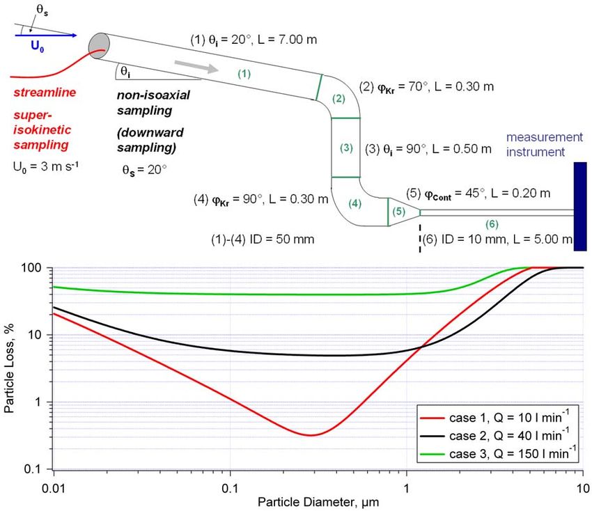
S.-L. von der Weiden et al.: Particle Loss Calculator                                                                                                  483

   These formulations are only valid for thin-walled sampling      where
probes for which the particle loss due to particle bounce on
the edge of the probe can be neglected. A sampling probe           Iv = 0.09(Stk cos(θS )(U − U0 )/U0 )0.3                                             (16)
can be regarded as thin-walled when the ratio of its outer to      for 0.25≤U0 /U ≤1 and Iv =0 otherwise,
inner diameter is less than 1.1 (Belyaev and Levin, 1972).                   p
Although different relationships are available for blunt sam-      Iw ⇓= Stk U0 /U sin(θS − α) sin((θS − α)/2)                                         (17)
plers, the use of blunt samplers should be avoided for most
applications.                                                      the direct impaction loss parameter for downward sampling
                                                                   (sampling probe faces upward),
2.2.2    Transmission efficiency of the sampling                               p
                                                                   Iw ⇑= Stk U0 /U sin(θS + α) sin((θS + α)/2)          (18)
         probe ηtrans
                                                                   the direct impaction loss parameter for upward sampling
The transmission efficiency ηtrans is the ratio of the aerosol     (sampling probe faces downward) and
particle number concentration behind the sampling probe to
the particle number concentration in front of the sampling         α = 12((1 − θS /90) − exp(−θS )).                                                   (19)
probe. The fractional particle loss is one minus the transmis-
sion efficiency. The particle loss in the sampling probe due       These equations are valid in the ranges 0.02≤Stk≤4,
to gravitational and inertial forces is expressed by the trans-    0.25≤U0 /U ≤4 and 0◦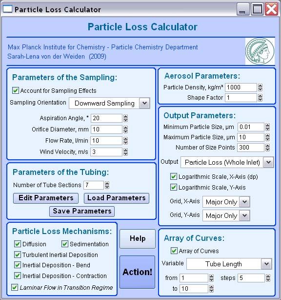
484                                                                            S.-L. von der Weiden et al.: Particle Loss Calculator

net transport of particles to the walls where they deposit. For          Under turbulent flow conditions the correlations of
laminar flow conditions in a tube, Willeke and Baron (2005)          Schwendiman et al. (1975) have to be used. Here the trans-
give an equation for the transport efficiency associated with        port efficiency due to sedimentation loss in a horizontal tube
diffusion:                                                           is:
ηdiff (da ) = exp(−ξ Sh)                                      (21)                         4Z           dLVts
                                                                     ηgrav (da ) = exp(−      ) = exp(−       )                   (26)
                                                                                            π            Q
where Sh is the Sherwood Number, ξ =πDL/Q, D is the
particle diffusion coefficient, L is the tube length and Q is        and for an inclined tube:
the flow rate.                                                                           4Z cos(θi )         dLVts cos(θi )
                                                                     ηgrav (da )=exp(−               )=exp(−                ). (27)
  For the Sherwood Number a formula by Holman (1972)                                         π                    Q
can be used:
                                                                     As in the laminar case the condition Vts sin(θi )/U 1 must
                          d
                0.0668    L   Re Sc            0.2672                be fulfilled.
Sh=3.66+                            =3.66+                    (22)
           1+0.04( Ld     Re Sc)2/3        ξ +0.10079 ξ 1/3
                                                                     2.3.3    Turbulent inertial deposition ηturb inert
where Re=ρf U d/µ is the Reynolds Flow Number, ρf is the
density of the air (the flow medium), U is the flow velocity         The turbulent inertial deposition is the inertial deposition loss
in the tube, d is the inner tube diameter and Sc=µ/(ρf D) is         of large particles due to the curved streamlines (eddies) in a
the Schmidt Number.                                                  turbulent flow. Large particles cannot follow these stream-
   If the flow in a tube is turbulent, the formula from Willeke      lines due to their high inertia and are deposited on the walls
and Baron (2005) (Eq. 21) is used with the experimentally            of the tube. Willeke and Baron (2005) give a relation for the
obtained Sherwood Number given by Friedlander and John-              transport efficiency associated with this effect:
stone (1957):
                                                                                                 π dLVt
                    7/8        1/3                                   ηturb inert (da ) = exp(−          )                         (28)
Sh = 0.0118 Re            Sc                                  (23)                                  Q

2.3.2   Sedimentation ηgrav                                          where
                                                                            (6×10⁻⁴ (0.0395 Stk Re3/4 )2 +2×10⁻⁸ Re)U
For particles having a diameter larger than about 0.5 µm,            Vt =                                                         (29)
                                                                                            5.03 Re1/8
gravitational forces cause particle loss. These particles set-
tle out due to their weight inside the tube, depositing on the       is the experimentally determined turbulent inertial deposition
lowermost surface as dictated by the acceleration of grav-           velocity. Equation 28 is valid in the turbulent flow regime up
ity. For laminar flow in a horizontal tube Fuchs (1964) and          to a Reynolds Number of 15 600 (Lee and Gieseke, 1994).
Thomas (1958) give the following relation, which is based
on a parabolic flow profile:                                         2.3.4    Inertial deposition: bend ηbend,inert

                   2 p                                              In a bend in tubing, the streamlines of the flow change their
ηgrav (da ) = 1 −      2  1 −  2/3 −  1/3 ·                       direction and large particles cannot follow them perfectly due
                  π
            p                                                       to their inertia. Whether they will be deposited on the walls
             1 −  2/3 + arcsin( 1/3 )                   (24)
                                                                     of the tubing as a result of their inability to follow flow lines
where =3/4Z and Z=LVts /(dU ). Z is the so called gravi-            depends on particle stopping distance. For laminar flow Pui
tational deposition parameter and Vts is the terminal settling       et al. (1987) give an empirical relation for the transport effi-
velocity of the particles.                                           ciency associated with this loss mechanism:
   If the tube is inclined with respect to horizontal by an angle                                  Stk 0.452 Stk +2.242 − 2 θKr
of inclination of θi , Heyder and Gebhart (1977) used exper-         ηbend,inert (da ) = (1 + (         )   0.171      ) π        (30)
                                                                                                  0.171
iments to derive a modified equation for the sedimentation
loss:                                                                where θKr is the angle of curvature of the bend in degrees.
                                                                        Pui et al. (1987) also provide an empirically determined
                    2  0p                                           relationship for the inertial particle loss in a bend in tubing
ηgrav (da ) = 1 −       2 k 1 − k 02/3 − k 01/3 ·
                    π                                               in turbulent flow:
            p
             1 − k 02/3 + arcsin(k 01/3 )                    (25)
                                                                     ηbend,inert (da ) = exp(−2.823 Stk θKr )                     (31)
where k 0 =    cos(θi ) and the condition Vts sin(θi )/U 1 must    The effect of the curvature ratio R0 on the inertial deposition
be satisfied.                                                        in a bend is insignificant for 5≤R0 ≤30 (Pui et al., 1987). The
                                                                     curvature ratio R0 is defined as the radius of the bend divided
                                                                     by the radius of the tube (Willeke and Baron, 2005).

Atmos. Meas. Tech., 2, 479–494, 2009                                                        www.atmos-meas-tech.net/2/479/2009/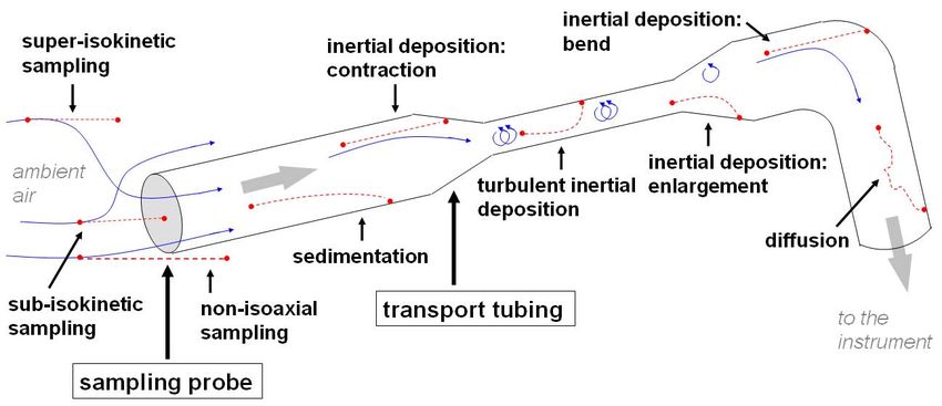
S.-L. von der Weiden et al.: Particle Loss Calculator                                                                                     485

2.3.5   Inertial deposition: contraction ηcont,inert                          the air inside the tube, aerosol particles get lost to the walls.
                                                                              In the opposite situation particle loss is reduced. Under most
In a contraction in tubing, there is also a change in the direc-              ambient aerosol measurement situations the temperature gra-
tion of the streamlines which larger particles cannot com-                    dient between the tube walls and the aerosol is smaller than
pletely follow. As a consequence, particles may deposit                       40 K and the particle loss due thermophoresis is negligible.
on the walls in front of the contraction. Muyshondt et al.                    This has been mathematically confirmed for several air ther-
(1996b) give a relationship for the transport efficiency ob-                  mal conductivities by the authors.
tained through experiments using particle collection on filters                  Diffusiophoresis: the deposition of aerosol particles due
both in front of and behind a contraction:                                    to concentration gradients can generally be neglected, if the
                                            1                                 sampled air is well mixed and the temperature gradient be-
ηcont,inert (da ) = 1 −                                            ,   (32)   tween aerosol and sampling lines is not too extreme. This is
                                     Stk(1−( A o
                                             Ai ))
                          1 + ( 3.14 exp(−0.0185           −1.24
                                                  θcont ) )                   important in order to avoid the condensation of gas molecules
                                                                              on the tubing walls, which would produce a concentration
which is valid in the ranges 0.001≤Stk(1−Ao /Ai )≤100 and                     gradient. These conditions are given under normal ambient
12◦ ≤θcont ≤90◦ . For this equation, θcont is the contraction                 aerosol measurement conditions (Willeke and Baron, 2005).
half-angle, Ai is the cross-sectional area in front of the con-                  Interception: interception is the process by which parti-
traction, and Ao is the cross-sectional area behind the con-                  cles travelling on streamlines sufficiently close to a tube wall
traction.                                                                     eventually come into contact with the wall, stick to it, and
                                                                              deposit. This effect is much smaller than other particle loss
2.3.6   Inertial deposition: enlargement
                                                                              processes if the dimensions of the particle are much smaller
In an enlargement in a piece of tubing, eddies form if the                    than the dimensions of the tube. In most inlet transport sit-
angle of enlargement is larger than 8◦ (or, in other words,                   uations this condition is fulfilled and interception can be ne-
if the half-angle is larger than 4◦ ) (Schade and Kunz, 1989).                glected (Willeke and Baron, 2005).
The eddies cause curved streamlines towards the tube walls                       Coagulation: coagulation is the conglomeration of many
and potentially causing particle deposition behind the en-                    smaller aerosol particles into fewer large ones. This process
largement. As there is no suitable equation describing this                   swiftly decreases the small aerosol particle number concen-
effect in the literature, care should be taken when designing                 tration while more slowly increasing the number concentra-
an inlet that angles of enlargement be kept small to avoid the                tion of large particles (Willeke and Baron, 2005). The aerosol
development of eddies (Willeke and Baron, 2005). The gen-                     particle loss due to coagulation can be neglected if particle
eral advice is to experimentally determine occurring particle                 concentrations are smaller than 100 000 particles per cm3
losses if it is not possible to avoid an enlargement in an inlet              and if the residence time of the aerosol in the sampling lines
system.                                                                       amounts to only a few seconds. This has been mathemati-
                                                                              cally confirmed by the authors.
2.3.7   Effects not considered in the Particle                                   Re-entrainment of deposited particles: re-entrainment of
        Loss Calculator                                                       particles is a not well-characterized process and should be
                                                                              avoided by cleaning the inlet lines, providing laminar flow
Electrostatic deposition: the loss of charged aerosol parti-                  conditions, reducing sedimentation of particles and mini-
cles due to electrostatic deposition is negligible if the sam-                mization of mechanical shock and vibration to the inlet sys-
pling lines are grounded and consist of conductive material                   tem (Willeke and Baron, 2005). It is important to consider,
(e.g. metal). Under these circumstances, no electrical field                  that re-entrained particles do not represent the current air
will exist in the interior of the tube (Faraday cage) and even                mass. Even if the actual losses of large particles are slightly
highly charged aerosol particles will not be electrostatically                lower due to re-entrainment, we think it is the best way to
deposited (Willeke and Baron, 2005). One exception to this                    assume a higher particle loss for large particles and not to
is in the case of unipolar charged aerosol particles where mu-                account for the re-entrainment of particles.
tual particle repulsion will produce a net flux of the particles
towards the walls causing deposition. Under most measure-                     3   Basic working principle of the Particle Loss Calculator
ment situations, aerosol particles are not unipolar charged
and this case can be neglected.                                               Generally, there are two approaches for calculation of parti-
   Thermophoresis: if a temperature gradient exists within                    cle losses in an inlet system. One approach involves the use
the tubing, a net flux of aerosol particles develops from hot                 of computational fluid dynamics (CFD) algorithms to numer-
to cold areas in a tube. This is due to the difference in mo-                 ically simulate the air flow and particle transport through the
mentum of the air molecules as a function of temperature.                     system. The other is the use of empirical and theoretically
On the hotter side, air molecules transfer more momentum                      derived formulas as described in Sect. 2 for individual tube
to the particles than on the colder side resulting in particle                sections and the calculation of the overall efficiency of the
transport towards the colder side. If the walls are colder than               total inlet system using Eq. (2).

www.atmos-meas-tech.net/2/479/2009/                                                                 Atmos. Meas. Tech., 2, 479–494, 2009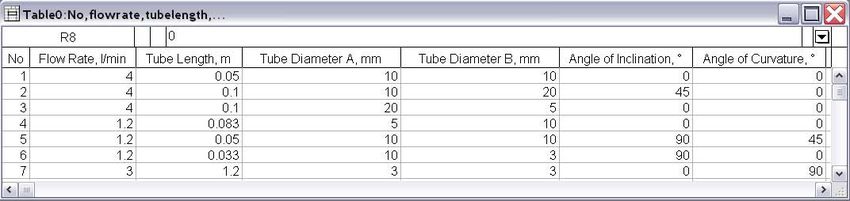
486                                                                       S.-L. von der Weiden et al.: Particle Loss Calculator

   CFD applications use numerical methods to solve complex        Loss Calculator was written using the scientific graphing and
coupled systems of equations (Navier-Stokes Equations) that       data analysis environment “IGOR Pro 6.04” (WaveMetrics,
describe fluid dynamical problems. Using such methods it          2009). It has a simple and clearly arranged user interface
is not only possible to calculate the gas flow field through      making the collated theoretical and experimental information
an aerosol inlet system, but also to determine aerosol parti-     found in a large selection of literature sources accessible to
cle distributions and particle trajectories. CFD calculations     all users. The results of the Particle Loss Calculator have
are the method of choice for the characterization of aircraft     also been experimentally validated.
inlets subject to high sampling velocities or other sampling
situations subject to similar conditions. The advantages of       3.1   Particle Loss Calculator (PLC)
this approach are, among other things, its wide range of ap-
plicability and the detailed representation of flow profiles in   The basic working principle of the Particle Loss Calcula-
tubing. Particle loss can be determined by the calculation of     tor is presented in Fig. 2. As described in Sect. 2, we sep-
particle trajectories and a detailed insight into the processes   arated the calculation of the total inlet sampling efficiency
occurring in a tube system is possible (CFD Review, 2009).        into two parts. The first part is the calculation of the sam-
   In spite of the power of this approach, one significant        pling efficiency of the sampling probe. This quantity is
disadvantage of computational fluid dynamics is the com-          composed of the aspiration and the transmission efficiency
plexity inherent in defining necessary input parameters (e.g.     (Eq. 3) and accounts only for effects associated with the sam-
the geometry of the calculated object and the calculation         pling of aerosol particles from ambient air into the tubing.
grid). Proper use of CFD software is only possible by trained     The second part of the calculation concerns transport effi-
users and is very time consuming to learn. In addition, the       ciency of aerosols through tubing to the measurement instru-
complexity of the numerical algorithms used in computation        ment. For calculation of transport efficiency, the inlet sys-
means that calculations themselves consume a great deal of        tem is separated into simple tube sections and the individ-
computational power. For these reasons, CFD calculations          ual transport efficiencies for each section are calculated for
are not well suited for quick, flexible estimates of particle     each loss mechanism (Eq. 20). The total inlet efficiency is
losses in an inlet system that are routinely encountered when     the combination of the sampling efficiency of the sampling
designing measurement systems. Furthermore, Tian and Ah-          probe and the transport efficiency through the transport lines
madi (2006) have shown that CFD calculations of particle          (Eq. 2). All calculations are performed for each particle size
losses occurring during turbulent aerosol sampling and trans-     in a user selectable size range and in user selectable size
port are often not reliable. Whereas the equations imple-         steps to achieve a size-resolved quantity. The Particle Loss
mented in the PLC are the results of experiments done with        Calculator can be set to calculate the efficiency of either one
turbulent flows, so they can be assumed to be more reliable       of these processes or the combination of both (overall effi-
to correctly describe the influence of turbulent sampling and     ciency/inlet efficiency).
transport.                                                           The user interface of the resulting software Particle Loss
   The use of empirical and theoretically derived formulas        Calculator is presented in Fig. 3. Six boxes logically orga-
was the method of choice for the Particle Loss Calculator to      nize the input parameters that must be entered to perform the
make calculations for arbitrary inlet systems accessible for      calculation. The “Parameters of the Sampling”-box is used
those not trained in CFD. This approach has already been          to define the variables for the computation of the inlet sam-
applied in the “AeroCalc” collection of Excel spreadsheets        pling efficiency. To perform such a calculation, the “Account
(Willeke and Baron, 2005). These spreadsheets contain more        for Sampling Effects”-check box must be activated. Other-
than 100 equations, largely detailed in Willeke and Baron         wise, when the “Action”-button is pressed, a warning text
(2005) and Hinds (1998), for the calculation of aerosol pa-       appears. Parameters used for the calculation of the inlet sam-
rameters like the air viscosity, the slip correction factor and   pling efficiency are the “Sampling Orientation”, the “Aspira-
the particle relaxation time. Using these spreadsheets, it        tion Angle”, the “Orifice Diameter”, the “Flow Rate” and the
is also possible to calculate particle losses in aerosol inlet    “Wind Velocity”. The sampling orientation of the inlet can
systems by combining appropriate formulas. Kumar et al.           be set as horizontal, upward (the aerosol is drawn from high
(2008) also used this approach, when they compared mea-           to low into the tube) or downward (the aerosol is drawn from
surements of ultrafine particle loss to theoretical determi-      low to high into the tube). The aspiration angle (in degrees)
nations based on the laminar flow model of Gormley and            gives the deviation of the sampling probe direction from the
Kennedy (1949) and the turbulent flow model of Wells and          wind direction (regardless of whether the derivation is in hor-
Chamberlain (1967).                                               izontal or vertical direction). The orifice diameter in mm is
   While “AeroCalc” is a multifunctional tool for the calcu-      the inner diameter of the tube opening, at the point where
lation of a large variety of aerosol parameters, the Particle     the aerosol enters the tubing. The flow rate in l min−1 is that
Loss Calculator is specially designed to streamline the com-      measured in the first tube section immediately downstream
bination of these calculations for efficient estimation of par-   of the orifice, and the wind velocity in m s−1 is the speed of
ticle losses in arbitrary aerosol inlet systems. The Particle     the surrounding air in relation to the sampling probe.

Atmos. Meas. Tech., 2, 479–494, 2009                                                    www.atmos-meas-tech.net/2/479/2009/
S.-L. von der Weiden et al.: Particle Loss Calculator                                                                                 487

Fig. 2. Basic working principle of the Particle Loss Calculator. In the green input boxes the variables in brackets are calculated from the
respective listed parameters, the variables without brackets are the listed parameters itself.

   It is important to note that the orifice diameter and the flow
rate required to calculate inlet sampling effects are also used
as parameters for calculating transport efficiency in the first
tube section. If these two parameters of the sampling probe
are different from the values set for the first tube section, an
error message is displayed.

   The “Parameters of the Tubing”-box contains necessary
input for calculation of the transport efficiency. First, the
user sets the number of tubing sections to be used for the cal-
culation (maximum 100). For this software, a tubing section
is defined according to constant parameters, e.g. a straight
tube or a bend of a certain angle. Any time one of the dimen-
sions of the tubing of an inlet changes, a new tubing section
must be started. After selecting the number of sections, the
user can choose to load or edit the parameters by clicking the
corresponding button. These buttons call a table containing
the parameters of the tube sections (see Fig. 4). The first line
of the table contains the parameters of the first tubing section
for the calculation of the transport efficiency, the second line
those of the second tubing section and so on. The follow-
ing parameters have to be set for each tube section: “Flow
Rate”, “Tube Length”, “Tube Diameter A”, “Tube Diameter
B”, “Angle of Inclination” and “Angle of Curvature”. The
unit of the flow rate is l min−1 , the tube length is in m, the di-
ameters are in mm and the angles are in degrees. The “Tube
                                                                        Fig. 3. User interface of the Particle Loss Calculator.
Diameter A” is related to the inner tube diameter at the begin-
ning (the first part of the tube encountered by air as it flows
through the tube) of a tube section. “Tube Diameter B” is the

www.atmos-meas-tech.net/2/479/2009/                                                             Atmos. Meas. Tech., 2, 479–494, 2009
488 S.-L. von der Weiden et al.: Particle Loss Calculator
inner diameter of the end (the last part of the tube encoun- can be used to determine optimum parameters of an inlet sys-
tered by air as it flows through the tube) of a tube section. tem during the design phase. One of several variables affect-
In the case of an enlargement or a contraction, the values for ing the sampling or the transportation processes can be varied
“A” and “B” will be different. For a straight tube section both in an user-selectable number of steps. The user sets the start
diameters “A” and “B” are the same. The angle of inclination (“from”) and the end (“to”) value of the respective variable.
is defined with respect to the horizontal plane. The angle For such calculations, the aspiration angle, the orifice diam-
of enlargement or contraction is calculated depending on the eter, the flow rate and the wind velocity can be varied. These
“Tube Diameter A”, the “Tube Diameter B” and the “Tube quantities are marked with an “(S)” in the “Variable” menu.
Length”. As discussed previously, particle loss due to devel- If one of them is chosen, the calculated quantity (Output Pa-
oping eddies in an enlargement with an angle larger than 4◦ rameters, “Output” menu) has to be the sampling efficiency
are not considered in the calculation. If this angle is too large, or the sampling loss. Otherwise a warning appears. For the
a message is displayed explaining that the calculated particle transport efficiency all parameters in the parameter table and
loss is underestimated. For later use of a tube system the pa- additionally the angle of contraction can be selected for an
rameters of the tubing can be saved with the corresponding array of curves. The angle of enlargement cannot be varied,
button. because the effects of an enlargement are not implemented
The “Particle Loss Mechanisms”-box allows the user to in the calculations. The determination of an array of curves
choose which of the implemented mechanisms are included is possible only for a single tube section (or inlet sampling
in the calculation. These mechanisms are diffusion, sedimen- conditions) and the variables for this section have to be set in
tation, turbulent inertial deposition, inertial deposition in a the first row of the parameter table.
bend and inertial deposition in a contraction. The user can To support the user in applying the Particle Loss Calcula-
include any number or combination of these mechanisms in tor a detailed help text (“Help”-button) explains all functions
the calculation allowing either general estimates of transport and parameters of this software. Additionally, the software
losses or investigation of the contribution of individual mech- prints information in the status line concerning individual el-
anisms to the overall process. ements when the cursor is over the each of the six areas in
To enable calculations for the transition regime for which the panel. The calculation of sampling and transport losses
no relationships exist, the formulas for the laminar flow starts by pressing the “Action”-button at the bottom of the
regime can be extended to non-laminar conditions by check- panel. After a short time either the output window appears
ing the “Laminar Flow in Transition Regime”-box. A warn- displaying the chosen quantity as a function of particle diam-
ing text will appear in the output graph pointing out that eter or one of the mentioned notifications points out that an
these calculations are outside of the valid range for the input parameter is wrong.
relationships employed. If this option is not chosen and the The output graph can contain a blue dashed line, a red solid
flow conditions in one or more tube sections are in the tran- line or both to present the chosen quantity. If a blue dashed
sition regime, no calculation of the particle loss is possible line (in the legend shown as “X”) appears, one or more of the
and an appropriate warning will appear. formulas used are out of their validity range. The result of the
The “Aerosol Parameters”-box is used to define the parti- calculation is then an approximation. A red line (in the leg-
cle density and the shape factor for the aerosol to be sampled. end shown as “N”) indicates that all formulas are within their
The default value of the particle density is 1000 kg m−3 , cor- stated validity range. In practice, the result of a calculation is
responding to the density of water. The shape factor is 1 for often still useful even if a formula is used outside its limits of
spherical particles and larger than 1 for other shapes (Sein- validity. This is particularly true of the equations applying to
feld and Pandis, 2006). If the characteristics of the sampled inlet sampling effects which seem to have a narrower stated
aerosol particles are known, these parameters can be changed validity than is actually allowable.
appropriately.
The “Output Parameters”-box contains variables that de-
termine the appearance of the output window displaying cal- 4 Validation measurements
culated results. As mentioned above, the user can choose to
To verify the functionality and practicability of the Particle
calculate either individual loss processes or the combination
Loss Calculator, we compared experimentally determined
of all effects. In this window, the user selects which results
particle losses in several simple test tube systems to the re-
to display as well as the particle size range and number of
sults of the Particle Loss Calculator. For the calculations
steps within this range that should be displayed (“Number of
using the Particle Loss Calculator, all particle loss mecha-
Size Points”). The chosen quantity, either percent efficiency
nisms were selected and therefore tested.
or loss, is plotted on the y-axis versus the particle size in µm
on the x-axis.
The “Array of Curves”-box is used to set the parameters
required for the calculation of an array of curves with varia-
tion of one of the sampling or tubing parameters. This feature
Atmos. Meas. Tech., 2, 479–494, 2009 www.atmos-meas-tech.net/2/479/2009/S.-L. von der Weiden et al.: Particle Loss Calculator 489
Fig. 4. Table containing the parameters of the tubing.
4.1 Experimental setup for both OPCs and CPCs were confirmed at regular time in-
tervals over the course of validation measurements to verify
Experimentally determined particle losses were calculated their stability.
with the following equation: For small particles (0.5 µm) those of inertial deposition (for exam-
number conc. of particles at tube entrance
ple, in a bend) and sedimentation dominate the overall loss.
Two identical Condensation Particle Counters (CPCs, TSI, We experimentally determined the particle losses of small
model 3007) and Optical Particle Counters (OPCs, Grimm, particles for five different test tubes with different lengths,
model 1.109) were used for the detection of particles at tub- curvatures, and diameters. The particle losses of large parti-
ing entrances and exits in the size range from about 10 nm cles were determined for three different tubes, two designed
to 350 nm and 300 nm to 32 µm, respectively. To reliably de- mainly for impaction losses (large total angle of curvature
termine particle losses, the instruments were tested to deter- with short length) and one mainly for sedimentation losses
mine that they respond identically when measuring the same (large horizontal extension). The flow conditions in all ex-
aerosol. periments were in the laminar flow regime.
The CPCs measure the number of aerosol particles per
4.2 Results of the validation measurements
cm3 independent of size. To obtain size-resolved measure-
ments of particle loss using a CPC, monodisperse aerosol For the validation experiments for the diffusional loss cal-
particles having a variety of sizes must be generated and culations of small particles, we used stainless steel 1/4 inch
tested separately. For CPCs experiments, aerosol particles (ID=4.57 mm) and 1/2 inch (ID=10.00 mm) tubes of several
were generated using an atomizer spraying aqueous ammo- lengths at low flow velocities. The 1/4 inch tubes had lengths
nium sulfate solution. The emerging droplets were dried of 20.80 m, 10 m and 3 m and were coiled in several turns
in an aerosol dryer filled with silica gel and the remain- (up to 10). The experimentally determined particle losses
ing particles were led into a Differential Mobility Analyzer show similar trends to the calculated losses. However, in the
(DMA, TSI, model 3081) which was used to select particles size range from about 20 nm to 200 nm the measured particle
of specific sizes from the polydisperse aerosol. A compari- losses are higher than the calculated losses. Measurements
son of the CPCs sampling from the same aerosol showed a made with varying numbers of turns (0 up to 18 coils) of the
small difference in instrument response independent of par- tubes show that the difference between measured and cal-
ticle size. For all subsequent experiments, a correction factor culated losses depends on the angle of curvature. With an
of 1.0094 was used to scale the response of one of the CPCs increased number of turns, particle losses increased. Particle
such that it exactly matched the response of the second. loss due to inertial effects (e.g. in curves) is expected to be
The OPCs measure the aerosol particle concentration (par- negligible for small particles in a laminar flow in the range
ticles per liter) in 31 different size channels from particles tested. Nevertheless, these results show that geometry has
larger than 0.25 µm ranging to particles larger than 32 µm. a strong influence on the aerosol particle losses. The struc-
These two instruments were used to sample ambient air in a ture of the flow seems to depend not only on the Reynolds
variety of locations. Over the course of the measurements, Number, but also on the geometry of the tube, at least the ex-
there was large size dependent discrepancy between signals treme we tested. As such an effect is not implemented in the
(up to 40%) for the two OPCs although they were sampling calculation of particle losses, we do not recommend its use
the same aerosol. Using this data, we derived a size depen- for calculations involving extreme geometries. We advise to
dent correction factor with which to scale the results of one keep inlet designs simple (avoidance of extreme curvature)
instrument to match the other (see Table 1 correction fac- to avoid possible excessive particle losses.
tor for outdoor validation measurements). Correction factors
www.atmos-meas-tech.net/2/479/2009/ Atmos. Meas. Tech., 2, 479–494, 2009490 S.-L. von der Weiden et al.: Particle Loss Calculator
Table 1. Correction factor applied to one of the OPCs during the outdoor validation measurements.
Particle Size (µm)
0.265 0.290 0.325 0.375 0.425 0.475 0.54 0.615
0.675 0.750 0.900 1.150 1.450 1.800 2.250 2.750
3.250 4.500 5.750 7.000 8.000 9.250 11.250 13.750
16.250 18.750 22.500 27.500 31.000
Correction Factor
0.841 0.998 1.015 0.968 0.840 0.609 1.028 0.870
0.920 1.101 0.816 1.125 0.930 0.903 0.963 0.925
0.881 0.912 0.833 0.985 0.868 1 1 1
1 1 1 1 1
In order to further validate the Particle Loss Calculator,
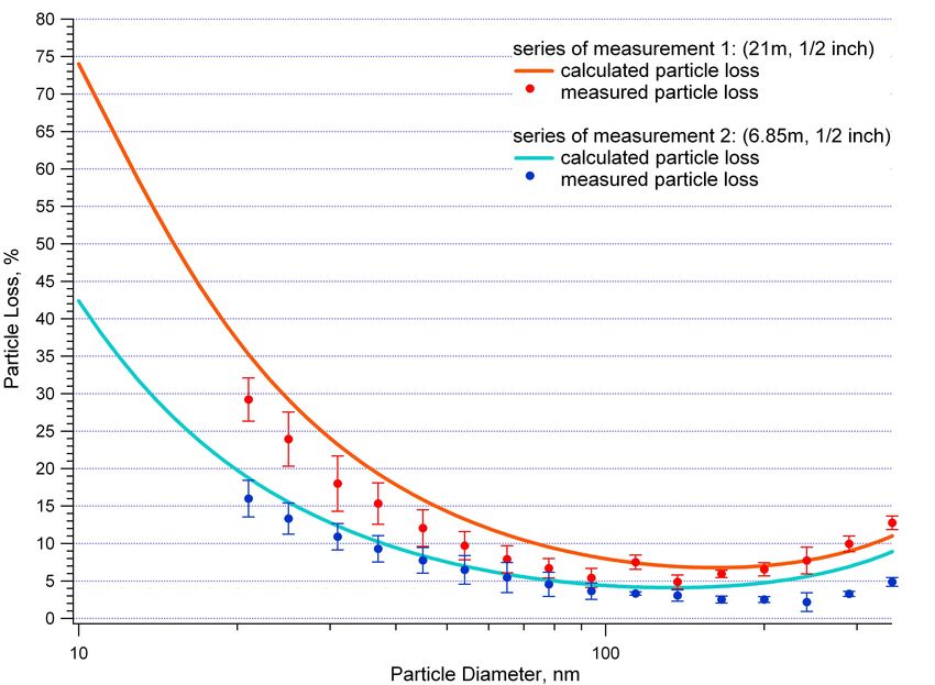
we used tubes with less extreme geometries. In Fig. 5 the
calculated and measured particle losses for two straight 1/2
inch tubes with lengths of 21 m and 6.85 m are shown. The
aerosol particle loss in percent is plotted on the y-axis ver-
sus the aerosol particle size (mobility diameter) in nm on the
x-axis. The points are the results of the measurements and
the lines are the calculated particle losses for the tube ge-
ometries used in the measurements. The error bars are the
standard deviation of a series of five measurements. The ex-
perimentally determined particle losses are consistent with
the calculated losses. This software tool can therefore be
assumed to function well in this size range and for simple
geometries where diffusion is the dominating particle loss
process. Below a particle size of about 20 nm, calculated
results cannot be validated as the DMA could not generate
reliable monodisperse aerosol below this size.
To validate the calculation of sedimentation and inertial Fig. 5. Measured and calculated particle losses in two 1/2 inch tubes
deposition for larger particles, three tubes with different ge- without curves and a length of 21 m (series of measurement 1, red
dots and line) and 6.85 m (series of measurement 2, blue dots and
ometries were tested. To obtain better counting statistics,
line).
some measurements were carried out near a busy street,
where larger concentrations of large aerosol particles were
available than in laboratory. Test tube configurations used shown here. However, results are comparable to those shown
for this measurement (1/4 inch-tube, total angle of curvature: in Fig. 6 with very good agreement between experimentally
720◦ , length: 0.35 m) are presented in Fig. 6 along with the determined and calculated particle losses. The Particle Loss
results of the tests. The line is the calculated particle loss Calculator appears to function well for this size range where
for the given tube geometry and the dots are the results of sedimentation and inertial deposition are the dominating par-
the measurements. Errors in the measurement are derived ticle loss mechanisms.
from counting statistics related to the total number of parti-
cles measured in each size channel. The measured particle
losses agree very well with the calculated losses up to a par- 5 Applications of the Particle Loss Calculator
ticle size of about 7 µm. The larger variation in the measured
particle losses between 200 nm and 2 µm may be related to In this section we present three applications demonstrating
unidentified external factors affecting determination of the the use and utility of the Particle Loss Calculator. Fig-
OPC correction factor. ure 7 depicts a virtual non-isoaxial and non-isokinetic sam-
The results for two other tubes, one designed for inertial pling system in conjunction with transport tubing designed
deposition (1/4 inch-tube, total angle of curvature: 1080◦ , for high particle losses during transport. The green numbers
length: 0.68 m) and the other designed for sedimentation demarcate individual tube sections used for the calculation.
losses (1/2 inch-tube, length: 0.66 m, no curvature), are not All other necessary parameters for the calculation with the
Atmos. Meas. Tech., 2, 479–494, 2009 www.atmos-meas-tech.net/2/479/2009/S.-L. von der Weiden et al.: Particle Loss Calculator 491
This example shows the utility of the Particle Loss Calcu-
lator for assessing the characteristics of an inlet system and
for adjusting sampling conditions to minimize losses. The
Particle Loss Calculator could further be used to correct re-
sults from existing systems to account for size dependent loss
processes or to estimate measurement errors.
As mentioned previously, the Particle Loss Calculator
was developed in order to optimize the aerosol inlet sys-
tem for the mobile laboratory MoLa of the Max Planck In-
stitute for Chemistry in Mainz, the goal being to minimiz-
ing particle losses across all size fractions to whatever ex-
tent possible and provide correction factors should losses be
non-negligible for a given size fraction or instrument. Sev-
eral boundary conditions existed for this task including ve-
hicle layout, already existing inlet ports and tubes, the char-
acteristics of the measurement instruments and the different
measurement conditions during stationary and mobile mea-
Fig. 6. Measured (red dots) and calculated (blue line) particle losses surements. Inlet efficiencies and particle losses had to be cal-
in a 1/4 inch tube designed for impaction losses in bends. culated numerous times to best optimize this system includ-
ing variations in tube routing, tube diameter, flow velocity,
arrangement of valves, inlet lines for each measurement in-
Particle Loss Calculator can also be taken from this figure.
strument, sampling probes for several driving speeds and the
This inlet system was purposely designed to demonstrate the
design of curved tube sections. Optimum particle loss in this
potential impact of poor inlet system design on aerosol sam-
case did not result in lowest losses everywhere, but rather a
pling. In the lower panel of Fig. 7, the size dependent par-
combination of low loss for the largest possible range of par-
ticle loss occurring in the virtual tube system for three dif-
ticle sizes within the measured size range of the individual
ferent flow conditions is shown. The particle loss in percent
instruments on board such that losses, when they did occur,
is plotted versus the particle diameter in µm. The red curve
had minimal impact.
(case 1) is the result using a flow rate of 10 l min−1 where
In Fig. 8 the calculated particle losses for three measure-
there is a laminar flow profile in all tube sections. Particle
ment instruments installed in MoLa (AMS, ELPI, TEOM)
losses are below 10% for a large size range and even drop un-
operated with the roof inlet are shown. The particle losses
der a value of 1% for particles between 100 nm and 600 nm.
in percent are plotted versus the particle diameter in µm and
Up to a particle size of a few µm the characteristics of the in-
the particle losses are shown across the measurement size
let system are acceptable for laminar flow conditions and the
range of the respective instrument. For the AMS the calcu-
results of an instrument measuring in this size range would
lated losses are below 2% over a wide size range, for the
likely be not negatively influenced.
ELPI below 10% and for the TEOM below 1%. The particle
The black curve (case 2) is the particle loss occurring in
losses are negligible for these three instruments when sam-
the inlet system if a flow rate of 40 l min−1 is used. In tube
pling through the MoLa roof inlet. The inlet losses for the
sections 1 to 5 laminar flow conditions prevail, while in the
other instruments and the other two inlet systems of MoLa
small diameter tube of section 6, the flow is turbulent. The
are of the same magnitude in as wide a size range as those
resulting particle losses are clearly higher than in case 1. For
shown in Fig. 8.
all particle diameters the losses are at least 5%. Only for par-
Yet another example of the use of the Particle Loss Cal-
ticles larger than 1 µm are the losses slightly smaller due to a
culator can be found in the publication of Sagharfifar et al.
shorter residence time in the inlet system reducing sedimen-
(2009). Here this software was applied to determine the par-
tation losses. In general, the sampling conditions are worse
ticle losses in the inlet system and the humidification cham-
in case 2 than in case 1 with non-negligible particle losses
ber of a modified condensation particle counter. The results
evident for all sizes.
of these calculations were used to estimate the overall error
Case 3 (green curve) depicts the sampling conditions pro-
of the instrument.
ducing that largest artifacts. Here, a flow rate of 150 l min−1
causes turbulent flow conditions in all tube sections. The re-
sulting particle losses are at least 40% for all particle sizes
6 Summary
and particles larger than 3 µm are not able to reach the mea-
surement instrument at all. Such sampling conditions should Accurate aerosol measurements taken under changing or
be avoided as meaningful measurements are impossible un- drastically variable sampling conditions place high demands
der these circumstances. on inlet systems used to sample aerosols. Optimization and
www.atmos-meas-tech.net/2/479/2009/ Atmos. Meas. Tech., 2, 479–494, 2009492 S.-L. von der Weiden et al.: Particle Loss Calculator
Fig. 7. Application example of the Particle Loss Calculator (virtual tube system not drawn to scale).
mance of existing aerosol inlet systems or development of
new ones. The Particle Loss Calculator helps to quickly de-
termine aerosol sampling efficiencies and particle transport
losses for arbitrary tubing systems as a function of particle
size. In developing this software, based on stepwise calcula-
tions for individual tube sections, we reviewed the processes
influencing the sampling and transport of aerosol particles
currently described in the literature and implemented those
processes strongly influencing particle loss under common
sampling situations. Where multiple parameterizations for a
loss process exist, the optimal parameterization was chosen
for implementation. This software was further validated by
comparison with experimentally determined particle losses
observed in several simple test systems. As long as tube ge-
ometries are not too extreme, calculations using the Particle
Loss Calculator program agree well with experiment.
Three examples demonstrate potential applications for the
Fig. 8. Calculated particle losses for three measurement instruments Particle Loss Calculator. Calculations involving a virtual in-
installed in MoLa (AMS, ELPI, TEOM) operated with the roof in- let system show the potentially deleterious effects of using
let. inlet systems with large and poorly characterized losses. In
addition, two real-world examples of inlet design are given.
One describes the utility of Particle Loss Calculator in de-
characterization of inlet systems is necessary to obtain repre- signing the inlet for the new MoLa mobile laboratory in
sentative aerosol sampling, to preserve the main characteris- Mainz and the second describes its use in characterizing the
tics of the ambient aerosol, and ensure scientifically signifi- inlet of a modified condensation particle counter.
cant results. The Particle Loss Calculator is a software under contin-
We developed a new Particle Loss Calculator (PLC) pro- uous development and suggestions for its improvement are
gram, based on both empirically and theoretically derived welcome.
relations that can be used for the assessment of the perfor-
Atmos. Meas. Tech., 2, 479–494, 2009 www.atmos-meas-tech.net/2/479/2009/You can also read