The dynamics of cooperation, power, and inequality in a group structured society
←
→
Page content transcription
If your browser does not render page correctly, please read the page content below
www.nature.com/scientificreports
OPEN The dynamics of cooperation,
power, and inequality
in a group‑structured society
Denis Tverskoi1,2*, Athmanathan Senthilnathan2,3 & Sergey Gavrilets1,2,3,4
Most human societies are characterized by the presence of different identity groups which cooperate
but also compete for resources and power. To deepen our understanding of the underlying social
dynamics, we model a society subdivided into groups with constant sizes and dynamically changing
powers. Both individuals within groups and groups themselves participate in collective actions. The
groups are also engaged in political contests over power which determines how jointly produced
resources are divided. Using analytical approximations and agent-based simulations, we show that the
model exhibits rich behavior characterized by multiple stable equilibria and, under some conditions,
non-equilibrium dynamics. We demonstrate that societies in which individuals act independently are
more stable than those in which actions of individuals are completely synchronized. We show that
mechanisms preventing politically powerful groups from bending the rules of competition in their
favor play a key role in promoting between-group cooperation and reducing inequality between
groups. We also show that small groups can be more successful in competition than large groups if
the jointly-produced goods are rivalrous and the potential benefit of cooperation is relatively small.
Otherwise large groups dominate. Overall our model contributes towards a better understanding
of the causes of variation between societies in terms of the economic and political inequality within
them.
Throughout our evolutionary history, humans have lived and interacted in groups. Group living implies coopera-
tion but also competition and conflicts between groupmates as well as conflicts between individual and group
interests, i.e. social d
ilemmas1–4. Such processes underlying group living are present at all levels of biological
organization5. In our close relatives chimpanzees, males within a band compete for mating opportunities but
cooperate in border patrols aiming to reduce the strength of a neighboring band6. Similarly, human groups
are engaged in cooperation but also in various types of conflicts including power struggles aiming to shape
between-group interactions and social institutions regulating them to their own advantage. As Aristotle put it,
“man is by nature a political animal”7. Examples of groups engaged both in cooperation and power conflicts
are common in modern human societies. These include social classes, political parties, and different ethnic,
religious, or regional groups.
Power struggles often lead to power inequality which then translates into economic inequality and other types
of inequality. Horizontal inequality, which is inequality between different identity groups in modern societies,
is an important topic of study in economics, sociology, social anthropology, and political s cience8–11. Horizontal
inequality negatively affects economic e fficiency12, the production of public g oods13 and government e fficiency14,
and it often leads to social instability and conflicts15. Inequality also negatively affect the well-being of citizens in
different ways especially when it becomes institutionalized (e.g., as studied in the Social Dominance Th eory16).
Between-group inequality affected the historical development and survival of many tribes, chiefdoms, states, and
empires17–19. To better understand these processes, we need to consider the dynamics of collective a ction4,20–27
in cooperation and conflict at multiple l evels5.
In the fields of biological and cultural evolution, there is now an extensive theory of “multilevel selection”
describing both within-group cooperation and between-group competition. The former is usually modeled by
linear public goods games (PGG). The latter is usually described by models of differential group survival adapted
from population genetics in which between-group interactions are i ndirect28–30 but some models consider direct
1
National Institute for Mathematical and Biological Synthesis, University of Tennessee, Knoxville, TN 37996,
USA. 2Center for the Dynamics of Social Complexity, University of Tennessee, Knoxville, TN 37996,
USA. 3Department of Ecology and Evolutionary Biology, University of Tennessee, Knoxville, TN 37996,
USA. 4Department of Mathematics, University of Tennessee, Knoxville, TN 37996, USA. *email: dtversko@
utk.edu
Scientific Reports | (2021) 11:18670 | https://doi.org/10.1038/s41598-021-97863-7 1
Vol.:(0123456789)
www.nature.com/scientificreports/
conflicts as well31–33. Usually competition at the group level happens globally, i.e. each group competes with all
other groups with equal i ntensity34–36, but see, e.g., a recent model37 in which groups interact locally.
There are a variety of models in economics that describe between-group contests. In these models, coopera-
tive groups secure a higher share of contested resource or have higher probabilities to win the c ontest38,39. Most
of these models implicitly equate the power of the group with its effort in the contest which controls the share
of the resource it secures. However there are also models of between-group conflict with a broader interpreta-
tion of power. For example, Refs.40–42 modeled contests for power between two or three factions in the society
(e.g. the elite, middle class, and commoners or the authoritarian government and the military or two political
groups), the winner of which determines the economic and political outcomes (e.g., democratic or despotic).
Ref.43 studied how the equilibrium contributions to conflict depend on the indices of inequality, fractionalization,
and polarization44 in the society. These studies highlight the political aspects of human societies which play an
important role in their dynamics.
Previous work based on non-cooperative game theory has largely ignored the possibility of between-group
cooperation. In a rare exception, Refs.45,46 studied a multilevel game in which individuals are engaged in a cascade
of different hierarchical PGGs. However there was no between-group competition in their models. There is also a
diversity of models from cooperative game theory focusing on coalition formation47. In these models, the power
of individual factions is constant and determined endogenously, while economic factors are usually disregarded.
Recently Ref.48 introduced a novel approach for modeling cooperation and conflict in a society composed
by multiple factions engaged in economic and political interactions. In their model, which follows the general
approach of Ref.49, factions are engaged in an economic game and a separate political game about power. Spe-
cifically, at each time step the factions first cooperate or defect in an economic collective goods game played
according to the current state of a dynamic set of rules. Then they participate in a contest for the power to
change the rules of the economic game to be played at the next time step, in terms of how the collective goods
are divided among the factions. This model was an extension of a m odel50 describing non-equilibrium dynamics
of resources and power in a society engaged in the redistribution of a fixed amount of resource. In Ref.48 model
there are three possible outcomes: complete loss of cooperation, stable hierarchy (where one faction persists on
top of the hierarchy with some fluctuations in the power of other factions), and continuous turnover (where
cycles of cooperation and defection are coupled with cycles in power and inequality). However their model as
well as that of Ref.50 described the processes of societal evolution only at a meso-scale51 and did not consider
individuals explicitly. Therefore, the model neglects the collective action problem at the within-faction level and
the effects of the group s ize20.
Here we seek to remove these limitations. Specifically, we investigate the joint dynamics of three important
processes: within-group cooperation in production of public goods, between-group cooperation in production
of collective club goods (i.e., collective goods which are excluded from non-cooperating groups), and between-
group contest for the shares of jointly produced collective goods. In our framework, the collective action problem
is present at both within- and between-group levels. We assume that both individuals and groups are bounded
rational: they use myopic best response (with errors) to make their strategic decisions. We explicitly model the
dynamics of power focusing on the effects of a parameter measuring the strength of mechanisms preventing
politically powerful factions from bending the rules of competition in their own f avor40,41,52,53. We investigate
the effects of the degree of rivalry of the goods produced and allow for groups to have different sizes54. The latter
feature let us study Olson’s group-size paradox20,55–60. We aim to shed light on the following questions: when
and why cooperation emerge in group-structured societies? What are the causes of variation between societies
in terms of economic and political inequality within them? What are the effects of checks-and-balances pre-
venting politically powerful factions from bending the rules of competition in their own favor on cooperation
and inequality? How do the group size and within-group interactions affect cooperation and inequality at the
between-group level?
The model
We consider a society composed by G groups which interact repeatedly in time. Time is discrete. Let nj and fj
be the size and political power of group j (0 ≤ fj ≤ 1, fj = 1). Individuals within each group are engaged in
an economic game leading to the production of certain resources. Group members can divide these resources
among themselves equally or invest into another economic game at the level of groups. Groups also participate in
a separate political game about power to obtain a share of the jointly produced resources which then are divided
equally within each group. For example, from about 100 to 700 CE some societies in the Moche Valley, Peru,
were organized as a collection of interacting villages differing in power which depended on the role in religious
rituals. The villages cooperated in building irrigation systems but also competed over the extent of control over
them61. One can also think of any modern country where different states politically compete for shares of national
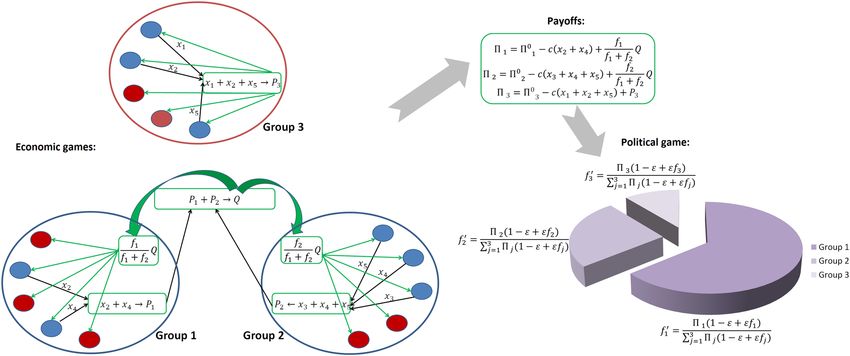
resources or jointly produced domestic products. Figure 1 illustrates the structure of our model.
Within‑group economic game. At the beginning of each time step, each individual i in a group j has
a baseline amount of resource π 0 > 0. First, each individual makes a decision to contribute ( xij = 1) or not
( xij = 0) to the group effort Xj = i xij . The cost of contribution is c (0 < c ≤ π 0). The resource Pj produced
by the group as a result of within-group cooperation is an increasing function of the combined effort Xj of group
members4:
Xj
Pj = B1 . (1)
Xj + X0
Scientific Reports | (2021) 11:18670 | https://doi.org/10.1038/s41598-021-97863-7 2
Vol:.(1234567890)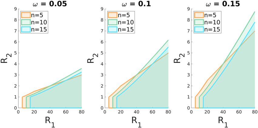
www.nature.com/scientificreports/
Figure 1. The model structure. Shown is an example of a society with three groups each with 5 individuals.
First, individuals and groups are engaged in economic games. Individuals cooperating in within-group game (in
blue) contribute to group production Pi; defecting individuals are shown in red. Groups 1 and 2 contribute their
production P1 and P2 to cooperate in the between-group game and produce resource Q to be divided according
to their relative power. Group 3 defects and just keeps the resource P3 it produced. After that groups contribute
the effort �i (1 − ε + εfi ) to a political game the result of which modifies their political power from fi to fi′.
Here B1 is the maximum possible benefit of the within-groups cooperation and X0 is a half-effort parameter
(which specifies the level of group effort at which Pj = B1 /2). Equation (1) describes a public good game with
non-linear production function and diminishing marginal return of group productivity62,63. Parameters B1 and
X0 can reflect the quality of the environment experienced by groups.
Between‑group economic game. After completion of within-group games, each group (or its repre-
sentative) decides on whether to keep the produced benefit (θj = 0) or invest it in between-group cooperation
(θj = 1). Cooperating groups can be viewed as a coalition of elites; defecting groups can be viewed as counter-
elites64. We assume that groups with Xj = 0 are never part of the elites.
Let C be the size of the coalition, i.e. the number of groups that have decided to participate in the between-
group game. Let Z = Pj be their combined contribution. We postulate that the resource Q produced as a result
of between-group cooperation is an increasing function of Z4:
Z
Q = B2 , (2)
Z + Z0
where B2 is the maximum possible benefit and Z0 is a half-effort parameter at the group level. Parameters B2 and
Z0 can reflect the quality of the environment experienced by the society. Note that both games utilize a nonlin-
ear production function used in earlier studies of “us vs. nature” and “us vs. them” g ames4, 65–67. This function
is more realistic than a standard linear production function in both capturing diminishing marginal return of
productivity and allowing for partial participation (i.e., a situation where cooperators and defectors coexist)
expected in many real-world situations.
A cooperating group j gets a share vj of the produced resource which is equal to its relative power within the
coalition:
fj
vj = , (3)
k fk
where the sum is over the set of all cooperating factions. In this model of “club goods”68, only the coalition of
elites share the amount of goods Q dividing them according to their power, whereas the counter-elites just keep
their own production Pj.
The total material payoff obtained by group j is thus
Pj , if the group defects
j = 0j − cXj + (4)
vj Q if the group cooperates.
where �0j = nj π 0 is the total baseline resource of group j.
After completion of the games, the resource obtained by each individual in group j represents a 1/nαj -share
of its group resource. Here parameter 0 ≤ α ≤ 1 characterizes the degree of rivalrousness of the g oods55,56. For
example, if α = 1, the goods are fully rival. In contrast, if α = 0, the goods are pure public. For α > 0 increas-
ing the size of the group decreases the individual’s share/value, while if α = 0, the individual’s share/value does
Scientific Reports | (2021) 11:18670 | https://doi.org/10.1038/s41598-021-97863-7 3
Vol.:(0123456789)www.nature.com/scientificreports/
not depend on the group size. Ref.69,70 show that many publicly provided goods exhibit a high degree of rivalry
(i.e., α is high).
Correspondingly, the payoff to each individual is
Pj /nαj , if the group defects
0
πij = π − cxj +
vj Q/nαj if the group cooperates. (5)
Below in illustrating our results, we will also use the normalized parameters
b1,j = B1 /nαj , b2 = B2 / nαj .
(6)
j
The former is the maximum benefit of within-group cooperation per individual. The latter is the maximum
benefit of between-group cooperation per individual while assuming an equal division of the jointly produced
reward.
Between‑group political game. After completion of economics games, all groups are engaged in a politi-
cal game that results in a modification of political powers. Specifically, we define the effective effort of group j in
the political game as
yj = �j (1 − ε + εfj ) (7)
and postulate that the group j power at the next time step is given by the Tullock contest success function : 38
y
j , if
′ yk > 0
fj = 1
yk (8)
G , otherwise.
The incumbency effect parameter ε controls the strength of dependence of yj on power fj ( 0 ≤ ε ≤ 1). If
ε = 0, then yj = j and only the amount of the faction’s material resource j matters; if ε = 1, then yj = j fj ,
so that the material resource and power combine multiplicatively in defining yj . The smaller this parameter is,
the stronger are the forces in the society (such as the rule of law, checks and balances, and democratic institu-
tions) preventing politically powerful factions from bending the rules of competition in their own favor71,72. With
larger values of ε, politically powerful factions manage to increase disproportionately their shares of resources.
Strategy revision and decision‑making. Each individual updates their strategy in the within-group
economic game randomly and independently with a fixed probability µ1. Each group updates its strategy in
the between-group economic game randomly and independently with a fixed probability µ2. Both individuals
and groups use myopic best response subject to random errors to maximize their material payoff. Specifically,
when making decisions, each updating individual always compares the expected payoffs of two actions ( x = 0
and x = 1) and chooses the action which gives the higher payoff (with precision as specified in the Quantum
Response Equilibrium approach73). Similarly, each updating group chooses the action, θ = 0 or θ = 1, which
gives the higher payoff. The decisions are made synchronously for all updating individuals first, then for all
updating groups. After that the power of groups is updated. In the main text, we focus on the case of infinite
precision = ∞.
All model parameters are assumed to be time-independent. Table S1 in the Supplementary Materials (SM)
summarizes the variables, functions, and constant parameters of our model.
Results
Our model exhibits a very rich behavior: it can have multiple simultaneously stable equilibria and also show
non-equilibrium dynamics. “Methods” section summarizes our analytical results on some symmetric equilibria.
Here we discuss more complex dynamics observed in numerical simulations. In our simulations, for generating
the initial distribution of power we use a “broken stick distribution”74,75, if groups have equal size; and assume
that initially groups have equal power, if they have different sizes. We assume that initially, each individual and
each group cooperate randomly and independently with probability 0.5. To estimate characteristics of long-term
dynamics, the model was run 100 (or 200) times for 4000 time steps and the statistics were computed over the
last 1000 time steps.
Groups with identical sizes. We start by assuming that groups have equal size n. In this case, two possible
types of dynamics are observed: equilibrium and non-equilibrium. We will describe them separately focusing
on the effects of parameters. Throughout we will assume that the ratio of the maximum group benefit B1 to the
group cost cX0 at half-effort R1 = B1 /(cX0 ) is sufficiently large so that each group has at least one cooperating
member. Here we discuss numerical results for the case of groups with n = 10 individuals. Our analytical results
and additional numerical simulations (Figs. S10–S12 in the SM) show that groups of other sizes have similar
behavior.
Equilibria. Convergence to an equilibrium is the most common type of dynamics. The structure of equilibria
is very complex: there are many of them and they can be locally stable simultaneously (see section 5.1 in the SM
and Fig. 9). These equilibria share some properties. Specifically, at equilibrium, all non-cooperating groups (i.e.
counter-elites) have the same number of contributing individuals and have the same power. Among cooperating
Scientific Reports | (2021) 11:18670 | https://doi.org/10.1038/s41598-021-97863-7 4
Vol:.(1234567890)www.nature.com/scientificreports/
8 10 1
8 0.8
6
6 0.6
C
X
4
f
4 0.4
2
2 0.2
0 0 0
0 0.1 0.2 0.3 0.4 0 0.1 0.2 0.3 0.4 0 0.1 0.2 0.3 0.4
(a) (b) (c)
8 10 1
8 0.8
6
6 0.6
C
4
X
f
4 0.4
2
2 0.2
0 0 0
0 0.1 0.2 0.3 0.4 0 0.1 0.2 0.3 0.4 0 0.1 0.2 0.3 0.4
(d) (e) (f)
Figure 2. Effects of the incumbency parameter ε on the number of cooperating groups C (a,d), the number
of cooperating individuals per group X (b,e) and group power f (c,f). First row of graphs: equilibria with just
one type of cooperating groups. Defecting groups are shown in blue symbols. Second row of graphs: equilibria
with dominant (violet symbols) and subordinate (golden symbols) cooperating groups. Curves show the
average values of corresponding characteristics. The equilibria illustrated in the top and the bottom rows are
simultaneously stable. Eight groups of the same size n = 10. Other parameters: b1 = 20, b2 = 10, α = 1, c = 1,
π 0 = 1, X0 = 5, Z0 = 50, µ1 = µ2 = 0.25. The results shown are based on 200 runs with 4000 time steps for
each parameter combination. The outcomes for each run are averages of the last 1000 time steps.
groups (i.e, elites), all groups can have the same number of cooperators and same power (equal elites) or there
can be just two types of groups, which we will call dominant and subordinate (non-equal elites). All dominant
groups have the same number of cooperating individuals and the same power. All subordinate groups also have
the same number of cooperating individuals and the same power which however is smaller than that of domi-
nant groups.
For small values of the incumbency parameter ε, there can be several stable equilibria with equal (Fig. 2a) and
non-equal elites (Fig. 2d). For intermediates values of ε, the number of stable equilibria can increase (Fig. 2a,d).
The number of cooperators X in a cooperating group can be either smaller or larger than that in a defecting group
(Fig. 2b,e). The number of cooperators X in subordinate cooperating groups can be either larger or smaller than
that in dominant groups (Fig. 2e). In general, non-cooperating groups are less powerful than dominant groups
(Fig. 2f). They are less powerful than subordinate groups, if the incumbency parameter ε and the benefit per
individual b2 are small; and more powerful than subordinate groups, if the incumbency parameter is relatively
large (Fig. 2f). Increasing the incumbency parameter ε increases power of cooperating groups relative to that of
non-cooperating groups in the equilibria of the first type (Fig. 2c). For additional examples see Figs. S5–S9 in
the SM. The resource Q produced in an equilibrium with C = G equal cooperating groups is large compared to
other equilibria. However, the maximum amount of Q is observed when there is one dominant group and G − 1
subordinate groups (see Fig. S13 in the SM).
Figure 2f shows that for relatively high values of ε, subordinate groups (marked by golden color) do not switch
to defection in spite of the fact that defecting groups (marked by blue color) have higher power. Because such
subordinate groups have a very low number of contributors (see Fig. 2e) simply defecting will only decrease their
power. To make defection pay, they would also need to increase the number of contributors. Planning two-steps
ahead however is not allowed within myopic best response updating we use here.
Non‑equilibrium dynamics. Non-equilibrium dynamics mostly happen when the incumbency parameter ε is
small and only within certain ranges of other parameters (for details see Figs. S14, S15 in the SM). In this regime
the cooperating coalition typically includes all groups but the number of cooperating individuals within groups
fluctuates. These fluctuations are coupled with fluctuations in power, which, in turn, lead to a turnover of domi-
Scientific Reports | (2021) 11:18670 | https://doi.org/10.1038/s41598-021-97863-7 5
Vol.:(0123456789)www.nature.com/scientificreports/
6
4
X
2
0
0 200 400 600 800
0.4
f
0.2
0
0 200 400 600 800
4
groups
3
2
1
0 200 400 600 800
t
Figure 3. An example of non-equilibrium dynamics. Top: the number of contributing individuals in each
group. Middle: faction powers. Bottom: groups cooperating at time t (i.e., those with θj = 1) are shown as black
pixels, while defecting groups (i.e., those with θj = 0) are shown as white pixels. Four groups of size n = 10 each.
Other parameters: b1 = 10, b2 = 26, ε = 0.1, c = 1, π 0 = 1, X0 = 5, Z0 = 50, µ1 = µ2 = 0.25.
nant groups. Below variable θj = 1 if group j cooperates in the coalition of “elites” and θj = 0 if not. An example
of non-equilibrium dynamics shown in Fig. 3.
Effects of parameters. We will focus on the number of cooperating groups C, the Gini index of inequality in
power among them I, and the standard deviation σ of cooperating group efforts. The Gini index is mathemati-
cally equivalent to half of the relative mean absolute difference.
Incumbency parameter ε. Increasing ε decreases the size C of the cooperative coalition (Fig. 4a) as low-power
groups do not receive large enough share of the jointly produced resource and leave the coalition. With suffi-
ciently large ε, only one group remains engaged in the between-group economic game. The inequality in power
and group efforts (Fig. 4a) among cooperating groups exhibit a hump-shaped dependence on ε. For more details
see Fig. S16 in the SM.
Benefit of within‑group cooperation b1. When b1 is small, increasing it increases between-group cooperation.
However, when b1 is high enough, the benefit of within-group cooperation exceeds that of between-group coop-
eration leading to a decline in cooperation (Fig. 4b). This process accelerates for higher ε (for more details see
Figs. S17–S19 from the SM). The inequality in power (Fig. 4b) and group efforts (Fig. 4b) among cooperating
groups exhibit a hump-shaped dependence on b1.
Benefit of between‑group cooperation b2. Effects of b2 depend on the incumbency parameter ε (see Figs. S20,
S21 in the SM). If ε is small, increasing b2 increases the number of cooperating groups C. There is no inequal-
ity between cooperating groups for small b2 but then it starts slowly increasing once b2 is sufficiently large. For
intermediate values of ε, increasing b2 first leads to an increase in the coalition size which then shrinks to just one
group as b2 becomes large enough (Fig. 4c). The inequality in power (Fig. 4c) and group efforts (Fig. 4c) among
cooperating groups exhibit a hump-shaped dependence on b2. With large ε, the coalition is never large as one of
its members quickly increases in power which causes all other groups to defect.
Effects of parameters Z0 , and G are discussed in the SM.
Groups with different sizes. Differences in group sizes have three structural effects. Increasing the group
size n: (1) increases the group’s total baseline amount of resource 0 making it more powerful, (2) decreases shares
of the resources 1/nα of each group member making cooperation more difficult (if α = 0); and (3) increases the
maximum possible group effort X. Because in our models within-group cooperation is typically low, the last
effect is weak. The trade-off between the first two effects drives the dynamics of the model. Below first we analyze
the average effects of various parameters while keeping the sizes of groups constant. Then we consider the effects
of changing the size of one group. At the end, we discuss non-equilibrium dynamics in more details.
Effects of parameters. We will consider four groups with 5, 10, 15 and 20 individuals, respectively. We assume
that all other parameters are identical between different groups and set groups’ initial power to 1/4.
If the benefit of between-group cooperation per individual b2 is small so that no between-group cooperation
is observed, smaller groups make larger efforts and have higher power in the case of rivalrous goods ( α = 1;
aradox20. In contrast, with non-rivalrous goods ( α = 0),
see Fig. 5). This is well in line with Olson’s group-size p
Scientific Reports | (2021) 11:18670 | https://doi.org/10.1038/s41598-021-97863-7 6
Vol:.(1234567890)www.nature.com/scientificreports/
5
5 0.5
C
I
0 0 0
0 0.2 0.4 0 0.2 0.4 0 0.2 0.4
(a) b1 = 20, b2 = 30
5
5 0.5
C
I
0 0 0
0 10 20 30 0 10 20 30 0 10 20 30
b1 b1 b1
(b) b2 = 20, ε = 0.3
8
6 0.6 G=2 4
G=4
C
4 0.4
I
G=8 2
2 0.2
0 0 0
0 10 20 30 0 10 20 30 0 10 20 30
b2 b2 b2
(c) b1 = 20, ε = 0.3
Figure 4. Effects of (a) the incumbency parameter ε; (b) the benefit parameter b1; and (c) the benefit parameter
b2 on the number of cooperating groups C, the Gini index of inequality I, and standard deviation of efforts σ
among them for different number of groups G. Groups of the same size n = 10 are considered. The shaded
areas shows the corresponding confidence intervals. Other parameters: α = 1, c = 1, π 0 = 1, X0 = 5, Z0 = 50,
µ1 = µ2 = 0.25. The figures show the averages and confidence intervals based on 100 runs each of 4000 time
steps for each parameter combination. Results in each run are averages based on the last 1000 of time steps.
efforts of smaller groups do not exceed efforts of larger groups and they obtain lower material payoffs and power
than larger groups (see Figs. S30, S31 in the SM). Increasing b2 brings more potential benefits of between-groups
cooperation. As a result, some groups switch to cooperation with the largest group typically being the first to
do so (see Fig. 5).
If ε is small, then all groups, one by one will switch to cooperation as b2 grows (see Fig. 5a) independently of
the degree of rivalrousness α (see Figs. S27–S31 in the SM). For intermediate and large values of ε, smaller groups
usually remain as defectors (see Fig. 5b,c). Larger groups are more successful within the cooperative coalition
(i.e., they have higher powers, obtain higher payoffs and are characterized by higher levels of a within-group
cooperation compared to smaller groups from the coalition) regardless of α (see Figs. S27–S31 in the SM). It
implies that high benefits of group interactions result in the disappearance of Olson’s group-size paradox inde-
pendently of rivalrousness.
Overall, the effects of other parameters are similar to those in models with equal group sizes (for details see
Fig. 5, Figs. S27–S31 from the SM). However, while in the former case which groups cooperate and which defect
is mostly determined by initial conditions and chance, in the later case it strongly depends on the group size.
Effect of changing the group size. Here we assume that there are 3 groups of 5, 10 and 15 individuals, respec-
tively, plus one additional focal group of size n which we will vary. For small and intermediate values of n, the
likelihood of cooperation for the focal group increases with n (see Fig. 6b) independently of rivalrousness (see
Figs. S32–S45 in the SM). Most often the largest group has the highest power within the cooperative coali-
tion regardless of α (see Figs. S32–S45, right panels). However, the effects of further increases in n depend
on the degree of rivalrousness. With non-rivalrous goods further increasing n promotes growth in the focal
group power, which, in turn, stimulates other groups to defect. This process is slowing down by a decrease in
the incumbency parameter. Eventually, for very high values of n, only the focal group remains engaged in the
between-group economic game. For more details see Figs. S40–S45 in the SM.
With rivalrous goods, further increases in n can lead to the loss of cooperation within the focal group (Figs. 6,
7b). Nevertheless, equilibria with the largest group characterized by the highest power within the coalition can
Scientific Reports | (2021) 11:18670 | https://doi.org/10.1038/s41598-021-97863-7 7
Vol.:(0123456789)www.nature.com/scientificreports/
10 1 1
5
10
15
X
5 0.5 0.5
f
20
0 0 0
0 20 40 0 20 40 0 20 40
b2 b2 b2
(a) ε = 0.1
10 1 1
X
5 0.5 0.5
f
0 0 0
0 20 40 0 20 40 0 20 40
b b b
2 2 2
(b) ε = 0.3
10 1 1
X
5 0.5 0.5
f
0 0 0
0 20 40 0 20 40 0 20 40
b2 b2 b2
(c) ε = 0.5
Figure 5. Effects of the benefit parameter b2 and the incumbency parameter ε on the average number of
contributing individuals X, the average cooperation status θ and average power f of each group. Groups with
5, 10, 15 and 20 individuals are considered. Baseline parameters: B1 = 100, α = 1, c = 1, π 0 = 1, X0 = 5,
Z0 = 50, µ1 = µ2 = 0.25. The figures show the averages based on 200 runs each of 4000 time steps for each
parameter combination. Results in each run are averages based on the last 1000 time steps.
still be observed (Figs. 6, 7a). Decreasing ε, Z0 and increasing B2 increase the value of the focal group size n for
which the likelihood of the focal group cooperation starts to decline with further increase in n; and the value
of the focal group size for which the focal group always defects with further increase in n. For more details see
Figs. S32–S39 in the SM.
Non‑equilibrium dynamics. Here we illustrate two interesting types of non-equilibrium dynamics. The first
type occurs when the system repeatedly transitions between equilibria with C and C + 1 cooperative groups (see
Fig. 7d). In this regime, which is observed if ε is intermediate, a subordinate group in the coalition switches to
defection once its power becomes low enough. This causes a decline in the resource obtained by the dominant
group resulting in decreases in its power. Once it has become sufficiently low, the most powerful among the
defecting groups returns to the coalition and the process repeats.
The second type of non-equilibrium dynamics is observed if ε is small (see Fig. 7c) when all groups cooperate.
In these dynamics, the cooperating coalition typically includes all groups but their powers as well as the number
of cooperating individuals within each of them fluctuate. This regime is similar to that observed if groups have
the same size. See Figs. S46–S49 in the SM for more details on the effects of various parameters.
Discussion
An important feature of many human societies is the existence of different identity groups (e.g., ethnic, cultural,
religious, political) which are engaged in economic cooperation but simultaneously are involved in competi-
tive interactions juggling for political power. These dynamics often lead to the emergence of different types of
(horizontal) inequalities between identity groups which often undermine economic developments and trigger
conflicts within society and its instability12–15. Understanding these processes is complicated by the fact that
Scientific Reports | (2021) 11:18670 | https://doi.org/10.1038/s41598-021-97863-7 8
Vol:.(1234567890)www.nature.com/scientificreports/
10 1 1
X1
5
f1
0.5
1
0.5
0 0 0
0 20 40 0 20 40 0 20 40
n n n
10 1 1
X2
5
f2
0.5
2
0.5
0 0 0
0 20 40 0 20 40 0 20 40
n n n
10 1 1
X3
5
3
f3
0.5 0.5
0 0 0
0 20 40 0 20 40 0 20 40
n n n
10 1 1
X4
4
5
f4
0.5 0.5
0 0 0
0 20 40 0 20 40 0 20 40
n n n
(a) (b) (c)
Figure 6. Effects of the group size n on the number of contributing individuals in a group X (a), the
cooperation status of a group θ (b) and group power f (c). Each point corresponds to an outcome of a particular
run. The values of θ larger than 0 but smaller than 1 indicate non-equilibrium dynamics. Characteristics of
groups with 5, 10, 15 and n individuals are marked by blue, red, yellow and violet colors respectively. Curves
show the average values of corresponding characteristics among all runs. Other parameters: B1 = 100,
B2 = 1500, ε = 0.5, α = 1, c = 1, π 0 = 1, X0 = 5, Z0 = 300, µ1 = µ2 = 0.25. These results are based on 100
runs with 4000 time steps for each parameter combination. The outcomes of each run are averages of the last
1000 time steps.
10
10
10
10
5
X
X
X
5
X
5 5
0 0 0 0
0 200 400 600 800 0 200 400 600 800 0 200 400 600 800 0 200 400 600 800
1 0.6 1
n=5 n=5 n=5 n=5
0.6 n=10 n=10 n=10 n=10
n=15
0.4 n=15 n=15
0.4 n=15
0.5 0.5
f
f
f
n=22
f
n=22 n=22 n=22
0.2 0.2
0 0 0 0
0 200 400 600 800 0 200 400 600 800 0 200 400 600 800 0 200 400 600 800
4 4 4 4
groups
groups
groups
groups
3 3 3 3
2 2 2 2
1 1 1 1
0 200 400 600 800 0 200 400 600 800 0 200 400 600 800 0 200 400 600 800
t t t t
(a) (b) (c) (d)
Figure 7. The dynamics of three groups of 5, 10, 15 individuals respectively and the focal group of n individuals
are illustrated. Examples of two main types of dynamics for high values of n are shown: (a) the focal group
cooperates and has the highest power among all groups; (b) there is no contributing individuals in the focal
group. Baseline parameters: n = 22, B1 = 100, B2 = 1500, α = 1, ε = 0.3, c = 1, π 0 = 1, X0 = 5, Z0 = 300,
µ1 = µ2 = 0.25. Examples of non-equilibrium dynamics for (c) ε = 0; and (d) ε = 0.3. Baseline parameters:
n = 20, B1 = 300, α = 1, b2 = 40, c = 1, π 0 = 1, X0 = 5, Z0 = 300, µ1 = µ2 = 0.25.
Scientific Reports | (2021) 11:18670 | https://doi.org/10.1038/s41598-021-97863-7 9
Vol.:(0123456789)www.nature.com/scientificreports/
individuals also interact at the within-group level. Our main goal here was to introduce a general theoretical
framework for addressing a number of important questions including: when are societies composed of groups
differing in power more (or less) stable? When is horizontal inequality high (or low)? When is cooperation and
production at the society level high (or low)?
Our model has several realistic features which have been largely neglected in earlier work. Most importantly
it considers the joint dynamics of cooperation and competition between different identity groups in the society
while explicitly accounting for individual behavior. We allowed for differences between groups in their sizes and
changing political power and explicitly focused on the effects of checks and balances mechanisms limiting the
ability of powerful groups to grab more power. We considered the effects of inequality, environmental conditions,
and rivalrousness of produced collective goods on cooperation and social dynamics.
Our models aim to capture important properties of historic and modern societies. For example, construction
of some large irrigation canals in the Moche Valley, Peru, involved multiple villages61. Maintaining the irrigation
system (e.g., doing regular cleaning) required a large collective e ffort76. Ref.77 suggested that villages competed
for the control over irrigation systems and the lands that they watered, and this control was performed in a
sophisticated power-based way via construction of temples. One can also think of any multi-ethnic modern
country where different ethnic groups politically compete for shares of national resources or jointly produced
domestic products. Examples include Mizrahi and Ashkenazi Jews ethno-national groups which cooperated to
built the Israel state but also competed for real and symbolic resources78; and Muslim and Christian communities
in Ghana which cooperate and collaborate for producing communal goods, but also compete with each other79.
In our model, the most common outcome of social dynamics is a stable society in which certain groups form
a cooperating coalition with a certain distribution of power while other groups remain outside of it. Continuous
cycles of cooperation and defection of groups, which were prevalent in Refs.48,50 (which neglected within-group
collective action problem and dynamics) never arose in our model. Although overall the spectrum of possible
dynamics observed in our model was broader than that in Refs.48,50, non-equilibrium dynamics were observed
under a much narrower range of parameters (see below). Therefore we can conclude that within-group dynamics
can stabilize the system’s behavior and that a society with individuals acting independently is more stable than
a society for which actions of individuals within groups are completely synchronized.
In our model, economic inequality is present at both individual and group levels. Inequality between indi-
viduals is a result of differences in individual efforts (with free-riders obtaining higher benefits) and differences
between the groups they belong to. The latter are caused by differences in baseline resources, group sizes, and their
power. We have shown that inequality among groups can be mitigated by decreasing the incumbency parameter
ε. In our model, a society consisting of equal cooperating groups can exist only if the incumbency parameter is
relatively low and groups have the same size. Such a society would produce large but not the maximum possible
amount of the resource Q. If groups are of equal size, the maximum amount of the resource is produced if all
groups in the society cooperate, but one of them is dominant in power and makes a disproportional high effort.
This effect of between-group differences is analogous to the effects of within-group heterogeneity on collective
action66.
We observed two different types of non-equilibrium regimes. In the first regime, observed for small val-
ues of the incumbency parameter ε, the cooperating coalition typically includes all groups but the number of
cooperating individuals within the groups fluctuate. These fluctuations are coupled with fluctuations in power,
which, in turn, may lead to the turnover of dominant groups. Turnover of governing parties in democratic states
can be viewed as an example of such dynamics. In the second regime, observed for intermediate values of the
incumbency parameter ε, one group persists at the top of the coalition with some fluctuations in the identity of
other coalition members. In this regime, the growing power of the dominant group forces subordinate groups
to leave the coalition decreasing production. Declining production decreases the power of the dominant group
which makes it beneficial for the most powerful among the defecting groups to return to the coalition thereby
completing the cycle.
Overall, the incumbency parameter ε plays a key role in our model. This parameter controls the extent to
which the differences in economic resources between groups are translated in the differences in power. We have
interpreted ε as a measure of the strength of democratic checks-and-balances or “the rule of law” mechanisms
working to prevent politically powerful factions from bending the rules of competition in their favor (smaller
values of ε implies stronger checks-and-balances mechanisms). We have found that reducing ε promotes coopera-
tion, reduces variation in power and, hence, mitigates between-group inequality. The effects of other parameters
strongly depend on ε as well. In particular, increasing potential benefits of between-group cooperation promotes
it only if the incumbency parameter is low. For intermediate values of ε, the cooperative coalition size C first
increases with the benefit of between-group cooperation but then shrinks to just one group as the benefits become
very large (see Fig. S20 in the SM). As a result, the model predicts that promoting cooperation and reducing
inequality via increased benefits of cooperation works properly only in societies with strong democratic checks-
and-balances. These results are well in line with the empirical literature: political institutions play a key role in
increasing economic efficiency and shaping economic g rowth80–83. Non-democratic societies with bad institutions
(e.g., institutions that work mostly for the benefit of the ruling elite) often exhibit very low levels of economic
growth coupled with deep economic crises and even civil wars84. However, some non-democratic regimes can
be very successful in terms of economic development (such as former dictatorships of the East Asian “tigers”,
such as Malaysia, Singapore, Taiwan, and South Korea). Their success arose partially due to strong nominally-
democratic institutions aiming to ensure the cooperation between elites and counter-elites81,84.
Differences in group sizes and their effects are related to the so called group-size paradox, i.e. the observa-
tion that larger groups can be less successful than smaller groups in collective actions due to increased free-
riding20,55. This paradox has been extensively studied for both within-group c ooperation85,86 and between-group
contests87,88. Here we considered the effects of group size on the group success in the context of more complex
Scientific Reports | (2021) 11:18670 | https://doi.org/10.1038/s41598-021-97863-7 10
Vol:.(1234567890)www.nature.com/scientificreports/
group interactions including both cooperation and competition. We have shown that differences in group sizes
have two main structural effects. First, larger groups have more baseline resources making them potentially
more powerful. Second, in larger groups individuals receive smaller shares of the collectively produced resources
making cooperation more difficult because of increased free-riding. The strength of the latter effect declines with
decreasing rivalrousness α of the goods. [When α is close to one, each individual’s share is inversely proportional
to the group size. In contrast, if α is close to zero, the amount of resources received by each individual does not
depend on its group’s size.] The interaction between the above two effects drives the dynamics of the model.
For groups not involved in between-group cooperation, smaller size leads to more resources (and power) if the
goods are rivalrous but less power and equal resources (compared to those produced by larger groups) if goods
are non-rivalrous. Similar results were obtained for a related model in Ref.56. For groups involved in between-
group cooperation, larger size most often leads to more resources and power for any degree of rivalrousness.
Nevertheless with fully rivalrous goods, cooperation in very large groups breaks down and such group withdraw
from between-group cooperation. This will also decrease their power.
There are a number of parallels between our model predictions and observations from real societies. Dif-
ferent stable states predicted in our model are similar to those found in some past and present societies. For
example, some alliances of Middle East tribes17 and cooperative structures among Native American Nations89
can be viewed as examples of equilibria with a relatively egalitarian coalition. Conversely, confederations of
Turco-Mongolin tribes with leading and subordinate t ribes17 can be treated as an illustration of equilibria with
high inequality between coalition members. The non-equilibrium dynamics (observed under some conditions
in our model) has been a focus of recent research on historical s ocieties19,50. The important role of social institu-
tions, and checks and balances preserving cooperation (which we explicitly modeled here via parameter ε) is
well appreciated in the social sciences. For example, Botswana has a very high per-capita growth rate compared
to other African countries. This can be explained by strong institutions that existed in Tswana tribes in the pre-
colonial period, aimed to maintain cooperation and resolve conflicts among t hem18. These institutions were
preserved and reinforced during history because of a relatively small effect of colonialism on Tswana tribes,
and due to the inclusive nature of these institutions with respect to other ethnic g roups90. See also the example
of the East Asia “tigers” briefly discussed above. Another interesting example related to our model are Pueblo
societies, some of which were organized as a collection of interacting clans differing in power which depended
on land-ownership and their role in religious rituals. The clans cooperated in the cultivation of the land but also
competed for control over it91. Under good environmental conditions social relationships between clans were
egalitarian and cooperative. However under bad conditions (e.g., rain or early frost) more powerful clans had
food and stayed in the village while less powerful clans had to go out to hunt and gather. In our model, deterio-
ration of environmental conditions can be captured by a decrease in the benefit parameter B2. Decreasing B2
decreases the size of the cooperative coalition if the incumbency parameter is relatively small, or the incumbency
parameter and the benefit parameter B2 are both intermediate (for more details see Figs. S20, S21 in the SM).
This prediction is well in line with the anthropological observations mentioned above.
Our hope is that future work will allow for some predictions of our model to be tested using proxies and data
collected from real societies. For example, the level of cooperation in the society can potentially be estimated
using GDP-type measures. There are also a number of ways to measure horizontal inequality12,92, while the
strength of checks and balances mechanisms can be estimated using data on the strength of democratic institu-
tions and similar measures from the World Values S urveys93.
Our model has a number of limitations. First, because of within-group free-riding, the levels of within-
group cooperation observed in our model are relatively low. In particular, only dominant groups can contain
relatively high number of cooperating individuals. However there is a number of additional mechanisms poten-
tially increasing within-group cooperation which we did not consider. These include reputation, punishment21,
22,25,94,95
, between-individual d ifferences65, and social n
orms67,96,97. Certain types of free-riding can be mitigated
if individuals update their strategies by using imitation or f oresight25–27 rather than the myopic best response we
used here. We anticipate that some equilibria we observed would not occur with foresight. An example is a stable
equilibrium where subordinate members of the coalition have lower power and payoffs than defecting groups. If
a subordinate group takes into account future actions of its members, it may be beneficial for it to switch to defec-
tion. Although that would reduce its immediate payoff, the future payoffs will be higher. Second, here we dealt
with well-defined and stable groups. However, the structure of social interactions can be much more complex.
For example, interactions between individuals can be represented as a multilayer network98, 99, where each layer
corresponds to a different type of interaction (e.g., social relationships, business collaborations, contacts via social
networks). Third, groups can also face additional costs of building a coalition. These costs are implicitly embed-
ded into our parameters (e.g., in the benefit parameter B2). However, the model can be generalized to capture
different forms of the coalition costs. Naturally, we anticipate that introducing additional costs will decrease
the tendency of groups to cooperate. Fourth, here we assume that groups cooperate to produce some collective
action as in “us versus nature” games66. However, many historic alliances were founded to win conflicts against
other societies. Describing such interactions could be done within the framework of “us versus them” g ame66 at
a new inter-society level. Fifth, the incumbency parameter by itself can be a multidimensional parameter rather
than a scalar, or it can be formed endogenously as a response to changes in the focal social system. Finally, in
our model individuals try to maximize their material payoffs. In real life situations, non-material factors (e.g.,
beliefs, conformity with group-members, injunctive norms or different rituals) can have a significant impact on
individual decision-making100,101. It would be also good to find a way for scaling up group sizes perhaps using
the mean field game theory m ethods102 as well as to add spatial structure which has been a focus of many studies
103–105
of cooperation . We leave these extensions and generalizations for future work.
Scientific Reports | (2021) 11:18670 | https://doi.org/10.1038/s41598-021-97863-7 11
Vol.:(0123456789)www.nature.com/scientificreports/
Figure 8. The equilibrium with no cooperating groups (C = 0) exists and is locally stable when the benefit-to-
cost ratios of the within-group game R1 and between-group game R2 lie in the corresponding shaded region for
different group sizes n and parameter ω. Other parameters: X0 = 5, α = 1.
Overall, our paper highlights the challenges of maintaining cooperation in complex societies and provides an
additional argument towards the importance of social institutions aiming to prevent politically powerful groups
from bending the rules of competition in their own favor.
Methods
A single group. Consider a single group of size n. Generalizing earlier results in Gavrilets and Shrestha26 we
find that there will be a positive effort X ∗ in the within-group game if b1 > c(1 + X0 ), that is, if the maximum
benefit of within-group cooperation b1 = B1 /nα is sufficiently large relative to individual cost c and the group’s
half-effort X0. Let
R1 = B1 /(cX0 ). (9a)
be the ratio of the maximum group benefit B1 to the group cost cX0 at half-effort. Group effort X ∗ at equilibrium
increases with R1 but naturally cannot exceed n. Specifically, X ∗ can be approximated (see the SM) as
R1 < nα ,
0, if �
∗
�
X = (9b)
�
R
min n, X0 ( nα1 − 1) , if R1 > nα .
In the SM we also show that if the goods produced are characterized by some rivalrousness (i.e., α > 0), then
under some conditions smaller groups will make a larger effort than larger groups (Fig. S1). This is an example
aradox20, 55–57.
of Olson’s group-size p
Symmetric equilibria. Here we focus on the existence and stability to small perturbations in power of
groups of symmetric equilibria with C cooperating groups which all are identical in their efforts and power
(see section Some equilibria in the SM). Moreover, we assume that each group contains at least one cooperating
individual. For equilibria with C < G , we will assume that R1 /nα > 1 so that each non-cooperating group has
individuals making a nonzero effort. In deriving our results we used an approximation which treats individual
contributions xi as continuous. This approach is justified by results in Gavrilets and Shrestha26 as well as by the
comparisons of our analytical with numerical results.
First, an equilibrium with no cooperating groups (with C = 0) exists if each group would not be motivated
to cooperate. This condition simplifies to
nα
R2 < 1 + ωR1 1 − , (10a)
R1
where
R2 = B2 /Z0 (10b)
is the benefit-to-cost ratio for the between-group game, and
cX0
ω= (10c)
Z0
is the ratio of the costs of groups in within- and between-group games. Thus the state with no between-group
cooperation exists only if the benefit-to-cost ratio R2 of the between-group game is sufficiently small relative to
that for the within-group game, R1. The upper bound on R2 declines with increasing the group size n and the
degree of rivalrousness α but increases with parameters ω and R1.
The above equilibrium is stable to small perturbations in groups’ power, if ε < 1. For more details see the
SM. Figure 8 illustrates the above results.
Scientific Reports | (2021) 11:18670 | https://doi.org/10.1038/s41598-021-97863-7 12
Vol:.(1234567890)www.nature.com/scientificreports/
Figure 9. The equilibrium with C (> 0) equal cooperating groups exists and is locally stable when the benefit-
to-cost ratio of the within-group game R1 and the incumbency parameter ε lie in the shaded regions for different
values of R2. Other parameters: ω = 0.1, X0 = 5, c = 1, Z0 = 50, π 0 = 1, α = 1, G = 8 and n = 10.
Second, consider an equilibrium with C > 0 of identical cooperating groups. At this equilibrium, the effort
of each cooperating group is
∗ X0 R1 R2
Xc = −1 , (11)
ωCR1 + 1 Cnα
which is positive, if R1 R2 > Cnα. Thus Xc∗ decreases with increasing n, ω , α, R1 and C. In contrast, Xc∗ increases
with increasing R2. The number of groups G has no effect on Xc∗.
Consider a general case, when the total material payoff to a cooperating group is higher than the total material
payoff to a defecting group (the opposite case is considered in Proposition 4 in the SM). An equilibrium with
C > 0 cooperating groups exists, if each cooperating group is not motivated to defect; and each non-cooperating
group is not motivated to cooperate (if C < G ). The former condition can be expanded to
2
α CR2 4
1
R1 < n 1+ 1+ 2 α 1− ,
4 C n ω R2
i.e., a cooperating group will not be interested in withdrawing from cooperation, if the benefit-to-cost ratio R1
for the within-group game is lower than a threshold which increases with increasing the benefit-to-cost ratio R2
for the between-group game. For more details see section Some equilibria in the SM.
The latter condition can be written as
ε > εmin ,
where the boundary εmin is defined implicitly by algebraic equations (for more details see section Some equilibria
and Proposition 2 in the SM). The above equilibrium is stable to small perturbations in groups’ power, if
ε < εmax ,
where the boundary εmax is defined implicitly by algebraic equations (for more details see section Some equilibria
and Proposition 3 in the SM).
Overall, we conclude that an equilibrium with C > 0 cooperating groups exists and is locally stable if the
incumbency parameter is within a certain range:
(εmin , εmax ), if C < G,
ε∈
[0, εmax ), if C = G.
Recall that the incumbency parameter ε affects the level of inequality within the society (since for high values
of the incumbency parameter ε factions with higher power have more opportunities to bend the rules of competi-
tion in their favor). Intuitively, having ε larger than a minimal value εmin prevents non-cooperating groups from
joining the coalition (because they will have low power and thus will not receive enough of jointly produced
resources). At the same time, having ε smaller than a maximum value εmax prevents inequality growth within
the coalition. Figure 9 illustrates these results (along with the results on the case when the total material payoff
to a cooperating group is lower than the total material payoff to a defecting group).
In the case of complete between-group cooperation (i.e. with C = G)
Scientific Reports | (2021) 11:18670 | https://doi.org/10.1038/s41598-021-97863-7 13
Vol.:(0123456789)You can also read