Coupling of a sediment diagenesis model (MEDUSA) and an Earth system model (CESM1.2): a contribution toward enhanced marine biogeochemical ...
←
→
Page content transcription
If your browser does not render page correctly, please read the page content below
Geosci. Model Dev., 13, 825–840, 2020
https://doi.org/10.5194/gmd-13-825-2020
© Author(s) 2020. This work is distributed under
the Creative Commons Attribution 4.0 License.

Coupling of a sediment diagenesis model (MEDUSA) and an Earth
system model (CESM1.2): a contribution toward enhanced marine
biogeochemical modelling and long-term climate simulations
Takasumi Kurahashi-Nakamura1 , André Paul1 , Guy Munhoven2 , Ute Merkel1 , and Michael Schulz1
1 MARUM     – Center for Marine Environmental Sciences and Faculty of Geosciences,
University of Bremen, Bremen, Germany
2 Laboratoire de Physique Atmosphérique et Planétaire, Université de Liège, Liège, Belgium

Correspondence: Takasumi Kurahashi-Nakamura (tkurahashi@marum.de)

Received: 20 August 2019 – Discussion started: 7 October 2019
Revised: 27 January 2020 – Accepted: 3 February – Published: 2 March 2020

Abstract. We developed a coupling scheme for the Com-           another measure of model performance. Second, in our ex-
munity Earth System Model version 1.2 (CESM1.2) and the         periments, the MEDUSA-coupled model and the uncoupled
Model of Early Diagenesis in the Upper Sediment of Ad-          model had a difference of 0.2 ‰ or larger in terms of δ 13 C
justable complexity (MEDUSA), and explored the effects          of bottom water over large areas, which implied a potentially
of the coupling on solid components in the upper sediment       significant model uncertainty for bottom seawater chemical
and on bottom seawater chemistry by comparing the coupled       composition due to a different way of sediment treatment.
model’s behaviour with that of the uncoupled CESM hav-          For example, an ocean model that does not treat sedimentary
ing a simplified treatment of sediment processes. CESM is       processes depending on the chemical composition of the am-
a fully coupled atmosphere–ocean–sea-ice–land model and         bient water can overestimate the amount of remineralization
its ocean component (the Parallel Ocean Program version         of organic matter in the upper sediment in an anoxic environ-
2; POP2) includes a biogeochemical component (the Bio-          ment, which would lead to lighter δ 13 C values in the bottom
geochemical Elemental Cycling model; BEC). MEDUSA               water. Such a model uncertainty would be a fundamental is-
was coupled to POP2 in an offline manner so that each of        sue for paleo model–data comparison often relying on data
the models ran separately and sequentially with regular ex-     derived from benthic foraminifera.
changes of necessary boundary condition fields. This devel-
opment was done with the ambitious aim of a future appli-
cation for long-term (spanning a full glacial cycle; i.e. ∼
105 years) climate simulations with a state-of-the-art com-     1   Introduction
prehensive climate model including the carbon cycle, and
was motivated by the fact that until now such simulations       For Earth system models, the simulation of biogeochemical
have been done only with less-complex climate models. We        cycles in the ocean is of fundamental importance. Simulat-
found that the sediment–model coupling already had non-         ing biogeochemistry is important for the projection of un-
negligible immediate advantages for ocean biogeochemistry       known (e.g. future) climate states in a prognostic way, be-
in millennial-timescale simulations. First, the MEDUSA-         cause the biogeochemical cycles play an active role in the
coupled CESM outperformed the uncoupled CESM in repro-          climate system by changing greenhouse-gas concentrations
ducing an observation-based global distribution of sediment     in the atmosphere particularly through the carbon cycle. Sec-
properties, especially for organic carbon and opal. Thus, the   ondly, biogeochemical tracers are an important indicator of
coupled model is expected to act as a better “bridge” between   water masses, and thus a measure of the model quality in
climate dynamics and sedimentary data, which will provide       representing ocean structures when comparing model states
                                                                with observations and reconstructions. The distribution of

Published by Copernicus Publications on behalf of the European Geosciences Union.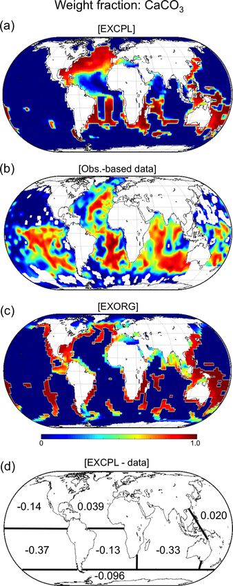
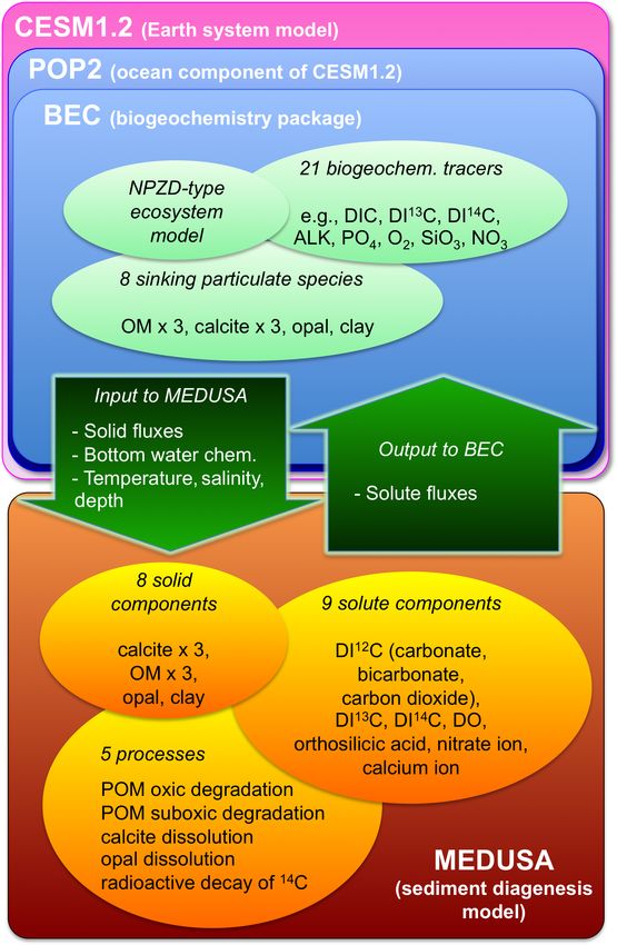
826                                                                T. Kurahashi-Nakamura et al.: CESM-MEDUSA coupling

biogeochemical matter in the ocean is determined by internal        2     Methods
processes (e.g. physical volume transport, mixing of seawa-
ter, and the biological pump) and processes at the upper and        2.1    Models
lower boundaries. The latter factors, boundary conditions in
terms of numerical modelling, consist of two aspects (e.g.          For the climate part of the coupled model, we employed
Kump et al., 2000; Ridgwell and Zeebe, 2005): the inflow            the Community Earth System Model (CESM; Hurrell et al.,
of matter as riverine input following chemical weathering           2013; version 1.2). CESM1.2 is a fully coupled atmosphere–
on land (i.e. the upper boundary condition) and the net out-        ocean–sea-ice–land model, and the ocean component is the
flow of marine matter at the ocean floor into sediments (i.e.       Parallel Ocean Program version 2 (POP2). In this study,
the lower boundary condition). This study focused on ex-            POP2 was configured to include the Biogeochemical El-
plicitly simulating the processes at the lower boundary, that       emental Cycling model (BEC; Moore et al., 2004, 2013;
is, the exchange of biogeochemical matter between the sea-          Lindsay et al., 2014). The BEC model is a nutrient–
water and ocean-floor sediments, which motivated the cou-           phytoplankton–zooplankton–detritus (NPZD)-type marine
pling of a climate model including an ocean biogeochem-             ecosystem model and contains a parameterized routine for
ical component and a process-based sediment model deal-             sinking processes of biological particles including particu-
ing with early diagenesis in sediments. Coupling a sediment         late organic matter (POM) with the “ballast effect” based
model is expected to lead to a better simulation of the seawa-      on Armstrong et al. (2002). The BEC model also includes a
ter isotopic composition especially for bottom water by pro-        highly simplified empirical treatment of dissolution of partic-
viding more realistic lower boundary conditions to an ocean         ulate matter at the ocean floor. For particulate organic carbon
model. This would be particularly important when the cli-           (POC) and opal, the amount of dissolved matter given back
mate model is applied to various climate states because a           to the seawater is empirically determined based on Dunne
substantial amount of paleoceanographic data is provided by         et al. (2007) for POC and Ragueneau et al. (2000) for opal,
isotopic measurements. In addition to the effects on seawater       and the residual matter corresponding to burial is simply lost
chemistry, the sediment model will allow to compare models          from the model domain. As to calcite, all particles that reach
and sedimentary records directly.                                   the ocean floor above a prescribed depth level (3300 m) are
   To simulate the sedimentary diagenesis, different mod-           lost from the model domain, and all particles dissolve below
elling approaches with a variety of complexity have been            that level. This original version of CESM with the simplified
used for paleoclimatological or global biogeochemical stud-         model for particle dissolution at the ocean floor was used for
ies (Soetaert et al., 2000; Hülse et al., 2017), which include a    comparison with the CESM coupled to our sediment module.
reflective boundary approach where all the sinking particles           The ocean model was also extended with the carbon-
that reach the sediments are dissolved in the deepest ocean         isotope component developed by Jahn et al. (2015), so that
grid cells (e.g. Yamanaka and Tajika, 1996; Marchal et al.,         we were able to simulate explicitly the carbon-isotope com-
1998), a vertically integrated reaction layer approach (e.g.        position of seawater, which is an important biogeochemical
Goddéris and Joachimski, 2004; Ridgwell and Hargreaves,             tracer from a paleoceanographic viewpoint. In this study, a
2007), and an approach with a vertically resolved transient         low-resolution setup of CESM following Shields et al. (2012)
diagenetic model (e.g. Heinze et al., 1999; Munhoven, 2007;         was used. The ocean component had a nominal 3◦ irregu-
Tschumi et al., 2011). In this study, we aim at advancing           lar horizontal grid with 60 layers in the vertical, while the
Earth system modelling by coupling a comprehensive cli-             atmosphere component, the Community Atmosphere Model
mate model, as opposed to an Earth system model of interme-         version 4 (CAM4), had a T31 spectral dynamical core (hori-
diate complexity (EMIC), including an ocean general circu-          zontal resolution of 3.75◦ ) with 26 layers in the vertical. The
lation model with a vertically resolved sediment model deal-        comparatively fine vertical resolution of POP2 (e.g. 200 to
ing with fully coupled reaction–transport equations. To our         250 m resolution for the depths deeper than 2000 m) allowed
knowledge, a fully coupled comprehensive climate model              a better representation of bottom-water properties, which was
including a sediment diagenesis model has been applied to           particularly important in this study’s context. Although only
millennial timescales only (Jungclaus et al., 2010). We are         the low-resolution case is shown in this study, a similar pro-
planning to apply such a model to timescales of tens of mil-        cedure will be applicable also to a higher resolution configu-
lennia with the goal of simulating glacial–interglacial vari-       ration for future applications.
ations. Here, we report on technical aspects of the coupling           For the sediment model part, we adopted the Model of
and assess the immediate influence of sedimentary processes         Early Diagenesis in the Upper Sediment of Adjustable com-
on the bottom-water chemistry. The assessment is important          plexity (MEDUSA; Munhoven, 2007). Note that this model
because it reveals possible model errors or biases of marine        is different from the marine ecosystem model with the same
biogeochemical simulations that depend on the treatment of          acronym (Yool et al., 2013). MEDUSA is a transient one-
sedimentary processes in a climate/ocean model. We also dis-        dimensional advection–diffusion–reaction model that, in its
cuss possible future applications of the coupled model for          original setup, describes the early diagenetic processes that
studies dealing with the long-term evolution of climate.            affect carbonates and organic matter (OM) in the surface

Geosci. Model Dev., 13, 825–840, 2020                                                  www.geosci-model-dev.net/13/825/2020/
T. Kurahashi-Nakamura et al.: CESM-MEDUSA coupling                                                                               827

sediment of 10 cm thickness (see also Fig. 2 in Munhoven,
2007). In the 10 cm thick surface “reactive” sediment, solids
are transported by bioturbation and advection, and solutes by
molecular diffusion. Solids that get advected across the lower
boundary of this 10 cm thick sediment get preserved (buried)
on a stack of 1 cm thick layers that can be interpreted as a
sediment core. The old deposits in the stack layers are treated
as being not reactive any longer in the model. The thickness
of the surface reactive layer is always kept at 10 cm, and in
case the net budget of solid material reduces the thickness to
less than 10 cm, some old material from the stack layers will
be “revived” to compensate for the loss in the reactive layer
and to keep the 10 cm thickness. In the coupled model, one
MEDUSA column was coupled to the deepest grid cell of
each POP2 water column and there was no lateral exchange
of information among the MEDUSA columns.
   In this study, MEDUSA was configured such that it treated
explicitly eight solid components and nine solute compo-
nents (Fig. 1), which is a substantial enhancement compared
to the original setup in Munhoven (2007). For the calcium-
carbonate species, only calcite was taken into consideration,
in line with the BEC model, although MEDUSA is able
to deal with aragonite as well. The time evolution of those
chemical species was governed by five processes (Fig. 1):
the oxic and suboxic degradation of POM, calcite dissolu-
tion, opal dissolution, and the radioactive decay of 14 C. Sub-
ject to boundary conditions (i.e. downward solid fluxes, so-
lute concentrations, and physical properties) at the top of the
sediment stack, the model forecasts the vertical profiles of
solid and solute components in 21 vertical layers. The so-
lute concentrations in the deepest grid cells of POP2 were         Figure 1. A schematic illustration of this study’s coupling scheme.
explicitly provided to MEDUSA except for calcium-ion con-          In the list of chemical species, “D” stands for “dissolved” and “I”
centration, which was empirically derived from the salinity.       for “inorganic”; for example, DO means dissolved oxygen and DIC
MEDUSA then returns solute fluxes at the sediment–water            dissolved inorganic carbon. OM stands for organic matter. Each of
interface back to the water column.                                OM and calcite components had three categories (for 12 C, 13 C, and
                                                                   14 C), and they were treated as separate tracers.

2.2   Coupling procedures

The communication between the two models was done in a               – Modifying POP2 involves
so-called “offline” manner; that is to say, we kept the executa-          – introduction of new variables for the matter ex-
bles of both models separate and exchanged necessary infor-                 changed with MEDUSA as shown in Fig. 1;
mation for their boundary conditions through file exchange.
                                                                          – adjusting writing/reading routines for boundary
We adopted the offline coupling considering the much longer
                                                                            conditions describing the additional variables;
characteristic timescale of the sediment model (e.g. a model
time step in Munhoven, 2007 is 100 years) compared to that                – modifying source/sink terms in the tracer prognos-
of the climate model. The offline method allowed manage-                    tic equations for the bottom grid cells of the ocean
ability of model development and maintenance while being                    model; and
physically credible at the same time. However, although we                – changing the formulation of the boundary condi-
could keep a substantial portion of the original structure of               tions at the ocean floor for the particulate matter.
each model especially for the technical procedures (e.g. in-
                                                                     – Modifying MEDUSA involves
terfaces to drive the models and input/output routines), it was
still required for us to make major alterations to both mod-              – creating writing/reading routines for boundary con-
els and to develop new routines to realize the coupling, as                 ditions; and
follows:                                                                  – unit conversion for variables to be exchanged with
                                                                            POP2.

www.geosci-model-dev.net/13/825/2020/                                                    Geosci. Model Dev., 13, 825–840, 2020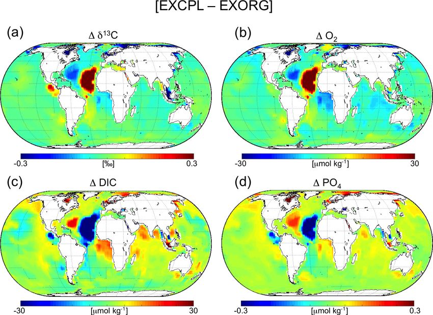
828                                                               T. Kurahashi-Nakamura et al.: CESM-MEDUSA coupling

  – Interfaces between the two models include                      (EXCPL). The second one was also run for 100 surface years
                                                                   but as a continuation of the “uncoupled” CESM spin-up run
       – format adjustment for the input/output files to uti-      (EXORG). The latter experiment was done to examine the ef-
         lize the existing schemes of both models as much          fect of the coupling of the process-based sediment model at
         as possible; and                                          millennial timescales. Again, it was not long enough for 14 C
       – automation of procedures: routines for each step of       to achieve reasonable steadiness. Both EXCPL and EXORG
         one-time coupling and a wrapper-level routine to          are designed as an “open” system. Both experiments have
         repeat them.                                              a common riverine-inflow field corresponding to the mod-
                                                                   ern river nutrient exports based on Seitzinger et al. (2010)
   For the coupling, CESM and MEDUSA were run sequen-              and Mayorga et al. (2010). On the other hand, the net flux
tially as in the coupling between the atmosphere and ocean         of matter through the lower boundary of the ocean domain is
components of CESM (Craig et al., 2012); that is to say, each      calculated by MEDUSA in EXCPL and by the parameterized
model was driven based on the state calculated by the other        burial treatment of BEC in EXORG.
in the previous integration period. Otherwise, we would have          In EXCPL, the two models communicated with each other
needed an iterative way to obtain a convergence of fluxes be-      10 times during the 100 years; that is, the coupling inter-
tween the two models that satisfied both of them for the same      val was 10 surface years for CESM, which was equivalent
time period. That would have required significantly more           to 200 years for the deepest ocean domain (i.e. deeper than
development work and would have increased computational            3500 m). At the end of each 10-surface-year CESM simu-
costs as well, and could be a subject of a future study.           lation, the annual mean values of the necessary variables
                                                                   from the last surface year were passed to MEDUSA. We ran
2.3   Experiments and analyses                                     MEDUSA for 200 years each time with a 10-year time step
                                                                   (see also the Supplement), and the model output at the last
First, we spun up the two models. CESM was initialized with        time step was used as input to CESM. Giving priority to the
the model state at the 507th year of the preindustrial run with    deepest ocean domain that occupies as much as ∼ 70 % of to-
the same resolution using the Community Climate System             tal ocean-floor area, we set the length of one MEDUSA run
Model version 4 (CCSM4, the model preceding CESM1.2)               to 200 years, which is in line with the length of the CESM
by Shields et al. (2012). Then the model was run for 200           integration for the deepest ocean domain.
years with an increased tracer time step for the deep ocean           Model performance was assessed by comparing the results
(Danabasoglu et al., 1996). The tracer time step (∼ 2 h for        to several observation-based datasets. The most straightfor-
the surface) was increased depending on the depth of the           ward benchmark quantities in the context of model–data
ocean: 5 times longer than at the surface for the depths from      comparison relevant for this study are the weight fractions
1000 to 2500 m, 10 times for 2500 to 3500 m, and 20 times          of the solid components in the upper sediment. Here, we fo-
for 3500 to 5500 m. Therefore, the length of the model run         cus on the surface sediment calcite, opal, and organic carbon
was equivalent to, for example, 4000 years for the very deep       (OC) for which Seiter et al. (2004) provide appropriate global
ocean. While most of the tracers came sufficiently close to        gridded maps. Another important parameter is the degree of
equilibrium, the model run was not long enough for 14 C,           saturation of seawater with respect to calcite defined by
which has the longer timescale of radioactive decay, and thus,
we do not discuss 14 C-related results in this study. By us-              [Ca2+ ][CO2−
                                                                                    3 ]
                                                                   =                   ,                                      (1)
ing the same acceleration method in all CESM experiments                      Kcalc
of this study, we assumed that the influence of the model
bias due to the acceleration (Danabasoglu, 2004) was mit-          where Kcalc denotes the solubility product of calcite.  > 1
igated as long as the differences among experiments were           in waters that are supersaturated with respect to calcite;  <
discussed. For this CESM spin-up, MEDUSA was not cou-              1 in waters that are undersaturated. We use the global map of
pled but the original empirical particle-dissolution treatment     Dunne et al. (2012) as a target dataset for the seafloor calcite
of the BEC model was used instead. After the CESM spin-            saturation state derived in our coupled model.
up, MEDUSA was initialized with a nominal uniform com-
position of the sediment-core-layer stack and pore water, and      3     Results
spun up for 105 years driven by the boundary conditions (i.e.
solid-particle fluxes and bottom-water chemical composition        3.1    Performance of the coupled model
in the deepest grid cells of POP2) derived from the spun-up
CESM model state.                                                  First, we evaluate the performance of the ocean component
   Following the spin-up sequence, we made two ex-                 of the coupled model based on the average over the last
periments. The first was a sequentially coupled CESM-              CESM run (i.e. 10 surface years) in EXCPL. The maximum
MEDUSA run for another 100 surface years with the same             transport of the Atlantic meridional overturning circulation
acceleration method for the deep ocean as described above          (AMOC) is 16.6 Sv (1 Sv = 106 m3 s−1 ), and the volume

Geosci. Model Dev., 13, 825–840, 2020                                                 www.geosci-model-dev.net/13/825/2020/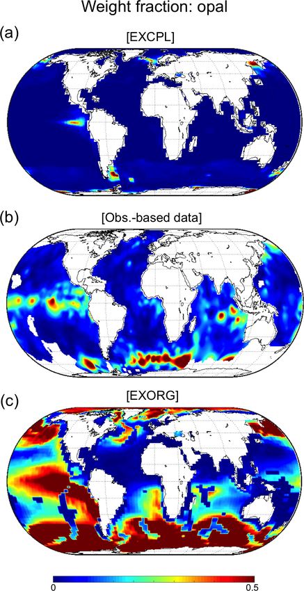
T. Kurahashi-Nakamura et al.: CESM-MEDUSA coupling 829
transport at 26.5◦ N (20◦ S) is 13.9 Sv (12.5 Sv), showing that
the physical ocean state is reasonably consistent with the es-
timates of the modern time-mean values given by several
data assimilation studies (Stammer et al., 2016). Given the
physical ocean state, the BEC model is able to reproduce the
observation-based estimates of various global-scale biogeo-
chemical quantities that are relevant to this study such as the
global export rates of POC and CaCO3 , and their deposition
rate at the ocean floor (Table 1).
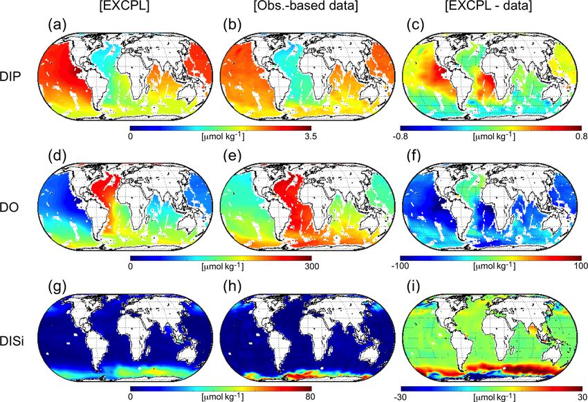
To evaluate the model performance of the sediment part
in the coupled model, we diagnostically obtained the weight
fraction of solid components in the upper sediment from
the outputs of MEDUSA. The weight fraction for calcite
(Fig. 2) is of special interest considering that it is closely con-
nected to the atmospheric CO2 level variations at the glacial–
interglacial timescale (e.g. Archer et al., 2000; Brovkin et al.,
2007, 2012; Munhoven, 2007). The global mean weight
fraction of calcite is 21 % at the last time step of the last
MEDUSA run in EXCPL and 38 % for the observation-based
global map (Seiter et al., 2004). Thus, the coupled model
underestimates the fraction of calcite preserved in the upper
sediments, which could be partly because the global supply
of calcite to the ocean floor itself is somewhat underestimated
(Table 1).
We also analysed the model performance in seven geo-
graphical regions (Fig. 2d). In five regions, the magnitudes
of the differences in the region-mean calcite weight fractions
between EXCPL and the observation-based data are smaller
than 0.15. In particular, small model–data mismatches are
realized in the North Atlantic, the western Pacific, and the
Southern Ocean.
In the North Atlantic, the spatial distributions are not con-
sistent, although the modelled region-mean weight fraction
is comparable to that derived from the data. For example, the
calcite weight fraction is significantly higher in the western
North Atlantic in the model results than in the observation-
based data by Seiter et al. (2004). A more recent observation-
based dataset (Dutkiewicz et al., 2015), however, indicates
that the major lithology of ocean-floor sediments is calcare-
ous matter in the western North Atlantic, the Caribbean Sea,
and the Gulf of Mexico. Although we cannot make a quanti- Figure 2. The weight fraction of the CaCO3 component in the upper
tative comparison between the newer dataset and our model sediments: (a) EXCPL, (b) the gridded map derived from observa-
tions (Seiter et al., 2004), and (c) EXORG. For EXCPL, the model
result because Dutkiewicz et al. (2015) does not provide the
state at the last time step of the last MEDUSA run is shown. The
weight fraction, the model result seems to be consistent with characteristic timescale of sediment-stack evolution is much longer
the recent data in those regions. The discrepancy between than 10 years, so that the weight fraction at the last time step suf-
the two observational datasets makes the interpretation of the ficiently represents the model state. For EXORG, we estimated the
model results in the western North Atlantic elusive. On the weight fraction by taking the ratio of the amount of solid matter that
other hand, it is also presumable that the model overestimates was excluded from the model ocean domain at the ocean floor based
the supply of calcite to the sediment in the midwest area of on the time averages over the last 10 surface years of the CESM run.
the North Atlantic because the modelled phosphate concen- (d) The breakdown of the EXCPL–data discrepancies into seven re-
tration in the surface water is higher than observed in that gions. The differences of the regional mean values for each domain
region (not shown), which would lead to an overestimation are shown (EXCPL minus data).
of biological production.
Noticeable discrepancies in the region-mean calcite
weight fractions are found in the eastern South Pacific and
www.geosci-model-dev.net/13/825/2020/ Geosci. Model Dev., 13, 825–840, 2020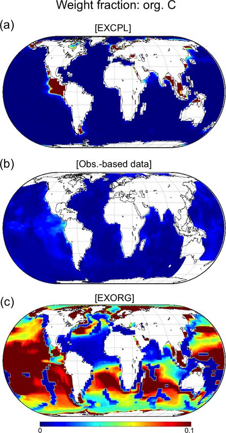
830                                                                   T. Kurahashi-Nakamura et al.: CESM-MEDUSA coupling

Table 1. Comparison of globally integrated biogeochemical quantities of this study with previous estimates available from observations. For
EXCPL, fluxes to allow consistent comparison with the previous estimates were calculated from the time averages over the last CESM run
(10 surface years).

                                                        This study (EXCPL)      Previous estimates
                   Atmospheric pCO2 (ppm)
                   Global mean                                         276.9    285.2 (Etheridge et al., 1996)
                   Net primary production (GtC yr−1 )
                                                                        59.4    48.5 (Field et al., 1998)
                                                                                49–60 (Carr et al., 2006)
                                                                                54 (Dunne et al., 2007)
                                                                                48.2 (Laws et al., 2011)
                                                                                55 (Ma et al., 2014)
                   POC (Gt yr−1 )
                   Export at 100 m                                        7.2   9.6 ± 3.6(Dunne et al., 2007)
                                                                                9.2–13.2 (Laws et al., 2011)
                                                                                4.0 (Henson et al., 2012)
                                                                                5.7 (Siegel et al., 2014)
                   Flux to ocean floor below 1000 m                     0.33    0.13 (Dunne et al., 2007)
                   between 60◦ N and 60◦ S
                   CaCO3 (GtC yr−1 )
                   Export at 100 m                                      0.95    1.1 ± 0.3(Lee, 2001)
                                                                                0.5–4.7 (Berelson et al., 2007)
                                                                                0.52 ± 0.15 (Dunne et al., 2007)
                                                                                0.72–1.05 (Battaglia et al., 2016)
                   Flux to ocean floor below 2000 m                     0.32    0.5 ± 0.3(Berelson et al., 2007)
                   Opal (Tmol yr−1 )
                   Export at 100 m                                      88.6    120 (Tréguer et al., 1995)
                                                                                70–100 (Gnanadesikan, 1999)
                                                                                101 ± 35(Dunne et al., 2007)
                                                                                105 (Tréguer and De La Rocha, 2013)
                   Flux to ocean floor                                  46.4    29.1 (Tréguer et al., 1995)
                                                                                22.1 (Dunne et al., 2007)
                                                                                78.8 (Tréguer and De La Rocha, 2013)

in the Indian Ocean. The Pacific anomaly, which shows a                 estimates  in that region, which affects the preservation of
too-low modelled calcite weight fraction, is caused by too-             calcite in the sediments.
corrosive bottom water. The  of the bottom water in that                  The simulated weight-fraction fields for OC and opal show
area is lower in the model results than that in the observation-        that they are minor components in general compared to cal-
based data (Fig. 3). The strongly undersaturated water having           cite, and that is consistent with the observation-based data
too-low pH is caused by the remineralization of an anoma-               (Figs. 5 and 6). In some regions, for example, in the east-
lous amount of OM, as indicated by the too-high concentra-              ern South Pacific (around 25◦ S, 110◦ W), the simulated OC
tion of phosphate in the deep water in this region (Fig. 4a–c)          weight fraction is lower than the observed OC fraction. This
and by too much consumption of oxygen as well (Fig. 4d–                 correlates with the underestimation of the calcite weight frac-
f), which are consistent with the too-high weight fraction of           tion (Fig. 2), which implies that less calcite burial may cause
OC in the eastern equatorial South Pacific (Fig. 5a). A sim-            a slower sedimentation rate, leading to a longer exposure of
ilar explanation is applicable to the Indian Ocean where the            OC to the pore water in the upper sediment and thus facili-
modelled calcite weight fraction is also lower than that in             tating its respiration. Although some more model–data mis-
the observation-based estimates; the model similarly under-             matches are visible mainly in coastal areas (for OC) and in

Geosci. Model Dev., 13, 825–840, 2020                                                       www.geosci-model-dev.net/13/825/2020/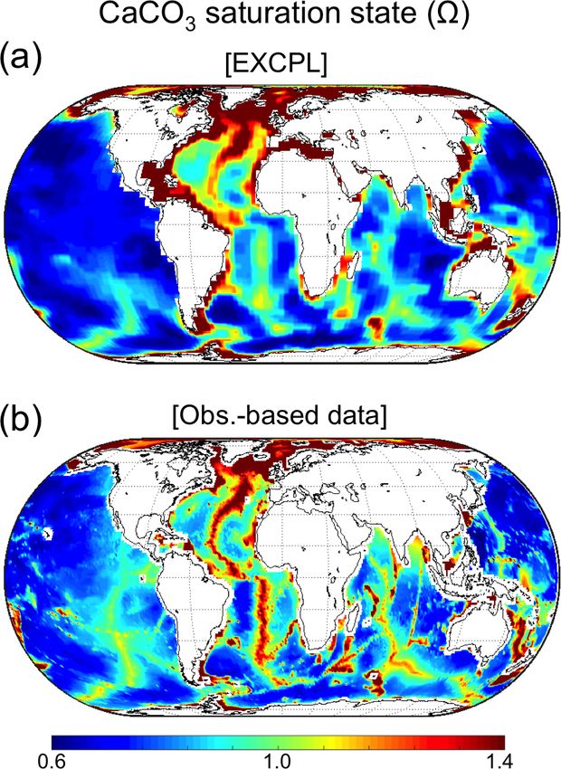
T. Kurahashi-Nakamura et al.: CESM-MEDUSA coupling                                                                                 831

                                                                       fraction of the solid components by taking the ratio of the
                                                                       amounts of each component and total solid matter that was
                                                                       excluded from the model ocean domain at the ocean floor,
                                                                       because the uncoupled CESM did not have explicit sediment
                                                                       stacks.
                                                                          The weight-fraction distribution for EXORG shows that
                                                                       the uncoupled model behaves differently. The rough feature
                                                                       of the global distribution of the calcite weight fraction in EX-
                                                                       ORG is similar to that in EXCPL or the observation-based
                                                                       data because of the appropriate depth of the prescribed lyso-
                                                                       cline (Fig. 2c). However, EXORG underestimates the frac-
                                                                       tion mainly in the Atlantic, presumably because the spatially
                                                                       constant lysocline is at shallower depths than observed in that
                                                                       area. On the other hand, the weight-fraction distributions for
                                                                       OC and opal show obvious discrepancies between the model
                                                                       results and the data. The weight fraction of OC in EXORG is
                                                                       unreasonably higher than that in the data in most regions of
                                                                       the global ocean and does not even approximately reproduce
                                                                       the observed spatial pattern (Fig. 5c). This is the case also
                                                                       for the opal weight fraction. The opal fraction in EXORG
                                                                       clearly deviates from the data, although it implies a higher
                                                                       fraction in the Southern Ocean and the eastern equatorial Pa-
                                                                       cific as suggested by the observations (Fig. 6c). Such large
                                                                       model errors would complicate the model–data comparison
Figure 3. Saturation state for calcite of the bottom seawater ().     for the upper sediment composition. Therefore, the coupling
(a) The model state in the deepest grid cells averaged over the last   of a more reliable sediment model like MEDUSA to CESM
CESM run (10 surface years) in EXCPL and (b) observation-based
                                                                       is essential for a straightforward comparison between model
estimates by Dunne et al. (2012).
                                                                       results and observations.
                                                                          The noticeable differences in the weight fractions of OC
the Southern Ocean (for opal), the performance of the cou-             and opal between EXCPL and EXORG are mostly caused by
pled model is remarkably better than that of the uncoupled             the different degrees of preservation of those two species in
model regarding the weight fraction of the two components              the upper sediment. Burial ratios (the ratios of burial amount
(see also Sect. 3.2).                                                  to the flux to the ocean bottom) of OM and opal calculated
   While the model performance with regard to the calcite              by MEDUSA in EXCPL are remarkably different from those
weight fraction may be improved to some extent by chang-               given by the highly simplified parameterization in the orig-
ing the model parameters of MEDUSA that govern the cal-                inal CESM (Fig. 7). In particular, the ratios in EXCPL are
cite dissolution rate, we keep the default parameter values for        significantly lower in low-flux locations, which means that
EXCPL in this study, which helps to assess the model per-              the difference will be larger in the open ocean. Depending on
formance in a standard setting. We judge the general model             whether OM or opal forms the major part of the total partic-
performance including the reproduction of the approximate              ulate flux (e.g. opal in the Southern Ocean), the difference in
pattern of global solid weight-fraction fields to be adequate          burial ratios will lead to substantial discrepancies in terms of
at this stage, at least for the following analyses and discussion      the weight fraction.
that does not require an accurate reproduction of the obser-              As to the ocean state, EXORG has large-scale proper-
vations.                                                               ties very similar to those for EXCPL; that is to say, in EX-
                                                                       ORG (EXCPL), the maximum strength of AMOC is 16.7 Sv
3.2   Comparison with the uncoupled model                              (16.6 Sv), the global export production is 8.1 GtC yr−1
                                                                       (8.1 GtC yr−1 ), and the global export rain ratio of CaCO3 is
Although the development of the coupled model in this study            0.13 (0.13), which suggests that the different treatment of
has been motivated by the aim of simulating the glacial–               the sedimentary processes does not have a remarkable ef-
interglacial variations including the marine carbon cycle as           fect on the overall physical and biogeochemical states of the
an open system (Sigman and Boyle, 2000), we find that the              ocean through the pCO2 and dynamics of the atmosphere
sediment–model coupling has non-negligible influences on               in our simulations. The two experiments are also compara-
ocean biogeochemistry even in millennial-timescale simula-             ble in terms of other globally integrated quantities such as
tions. The most prominent effect is found in the composition           the deposition fluxes of particulate matter and the total in-
of the upper sediment. For EXORG, we estimated the weight              ventories of biogeochemical tracers (Tables 2 and 3). This is

www.geosci-model-dev.net/13/825/2020/                                                       Geosci. Model Dev., 13, 825–840, 2020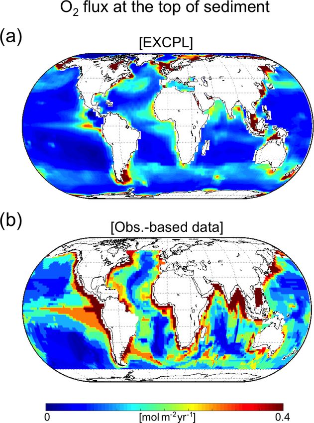
832                                                                      T. Kurahashi-Nakamura et al.: CESM-MEDUSA coupling

Figure 4. Distribution of marine biogeochemical tracers: (a–c) dissolved inorganic phosphate at the depth of 3000 m, (d–f) dissolved oxygen
at 3000 m, and (g–i) dissolved inorganic silicate at 10 m. The left column shows the time averages over the last CESM run (10 surface years)
in EXCPL, the centre shows observation-based data (GLODAPv2; Lauvset et al., 2016), and the right column shows the anomaly given by
model results minus the data.

Table 2. Globally integrated annual mean deposition flux of partic-       Table 3. Total inventories in the global ocean of DIC, ALK, and
ulate matter to the sediment and their burial flux (in parentheses) at    PO4 in EXCPL and EXORG. Values averaged over the last CESM
the end of EXCPL and EXORG.                                               run (10 surface years) are shown.

                                    EXCPL       EXORG                                                   EXCPL          EXORG
            POC (GtC yr−1 )             0.57        0.51                             DIC (GtC)      3.660 × 10⁴    3.657 × 10⁴
                                     (0.091)      (0.12)
                                                                                     ALK (Peq)      3.201 × 10³    3.201 × 10³
            CaCO3 (GtC yr−1 )           0.39        0.38
                                     (0.082)      (0.14)                             PO4 (Pmol)           2.948           2.923

            Opal (Tmol yr−1 )             46          45
                                      (0.72)        (3.4)
                                                                          1 indicates the difference given by EXCPL minus EXORG)
                                                                          in the deepest grid cells of the ocean model is ∼ 0.2 ‰ or
                                                                          larger in a substantial number of areas (Fig. 8a). Some of
reasonable because the timescale at which the sedimentary                 these areas correlate closely with the regions of high POC
processes alter the chemical state of the global ocean is very            flux to the sediment (Fig. 9) or high POC weight fraction
long (O(105 ) years) considering the slow turnover rate esti-             (Fig. 5a): along the east coast of the equatorial Pacific, along
mated from the size of the ocean carbon reservoir and the                 the west coast of the Pacific, and in the Arctic and Hudson
flux exchanged with the sediments (Ciais et al., 2013).                   Bay, for example. These regions (except for the eastern equa-
   However, the effect of the interactive coupling of                     torial Pacific) have negative 1δ 13 CDIC . The low δ 13 CDIC val-
MEDUSA on the local bottom-water chemistry is not neg-                    ues suggest that there is a larger amount of supply of “lighter”
ligible. The difference in δ 13 C of DIC (1δ 13 CDIC ; hereafter,         carbon from the sediment to the seawater in such regions,

Geosci. Model Dev., 13, 825–840, 2020                                                        www.geosci-model-dev.net/13/825/2020/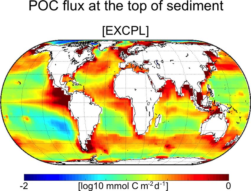
T. Kurahashi-Nakamura et al.: CESM-MEDUSA coupling                                                                               833

Figure 5. The weight fraction of the organic-carbon component in
the upper sediments: (a) EXCPL, (b) the gridded map derived from     Figure 6. The weight fraction of the opal component in the upper
observations (Seiter et al., 2004), and (c) EXORG. For EXCPL, the    sediments: (a) EXCPL, (b) the gridded map derived from observa-
model state at the last time step of the last MEDUSA run is shown.   tions (Seiter et al., 2004), and (c) EXORG. For EXCPL, the model
                                                                     state at the last time step of the last MEDUSA run is shown.

which results from the remineralization of a larger amount           by the reduced oxygen supply from the seawater (Fig. 10a)
of OM. This is supported by the large flux of oxygen from            due to the oxygen-depleted deep water (Fig. 4d), although
the seawater to the sediment in the same regions (Fig. 10a),         the model seems to underestimate the amount of oxygen
that could have been caused by a large vertical gradient of          available there as seen in comparisons with the correspond-
oxygen concentration, and is supported by the large DIC flux         ing observation-based fields (Figs. 10b and 4f). The limited
from the sediment to the seawater as well (Fig. 11). As a re-        amount of remineralization in the model result is also con-
sult, the distribution of 1O2 and 1DIC has a very similar            sistent with the very low DIC flux from the sediment to the
spatial pattern to that of 1δ 13 CDIC (Fig. 8b, c). This scenario    ocean (Fig. 11). That leads to more burial of lighter carbon
is also consistent with the 1PO4 distribution (Fig. 8d), which       (i.e. less supply of lighter carbon to the seawater), which re-
is anti-correlated with that of 1δ 13 CDIC .                         sults in the heavier δ 13 CDIC in the bottom water.
   A similar explanation, however, is not applicable to the             On the other hand, the remarkable dipole structure of the
eastern equatorial Pacific having positive 1δ 13 CDIC . The          1δ 13 CDIC field in the North Atlantic is not well correlated
seawater with larger δ 13 CDIC values suggests that there is         with the high-OM-flux regions (Fig. 9). Instead, it results
a smaller amount of supply of lighter carbon in spite of a           from water mass displacement caused by ocean circulation
large flux of POM to the sediment. In that region, the amount        changes rather than from the direct influence of the sediment,
of (oxic) remineralization in the upper sediment is limited          which shows that, although the overall sediment feedback on

www.geosci-model-dev.net/13/825/2020/                                                     Geosci. Model Dev., 13, 825–840, 2020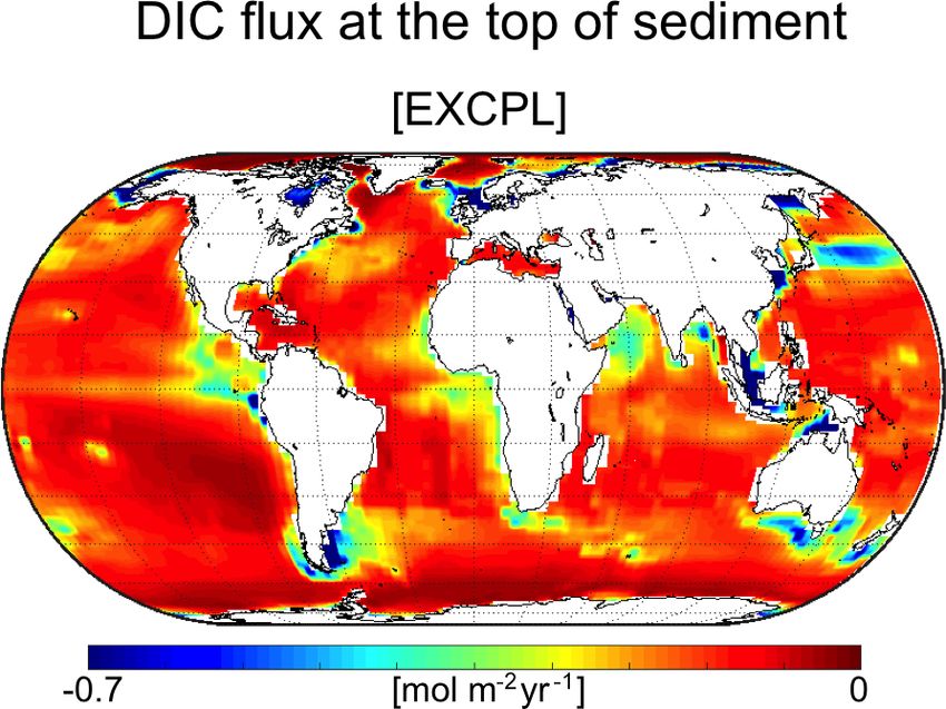
834                                                                    T. Kurahashi-Nakamura et al.: CESM-MEDUSA coupling

Figure 7. Sediment burial ratios versus the particulate flux to the ocean floor for (a) OC and (b) opal. The dots show the ratio at each grid
cell obtained in the last MEDUSA run for EXCPL. The solid lines indicate those given by the parameterized models in the original CESM
(BEC) based on Dunne et al. (2007) for OC and Ragueneau et al. (2000) for opal.

Figure 8. The difference in the chemical composition of the deepest grid cells between EXCPL and EXORG that was obtained from the time
averages over the last 10 surface years of the CESM run in each experiment. 1 indicates an anomaly given by EXCPL minus EXORG.

the physical ocean states is subtle as mentioned above, some             anomaly in the eastern North Atlantic is caused by the dif-
local effects are clearly visible. The negative anomaly of               ference in the strength of the northward current along the
δ 13 CDIC in the western North Atlantic is caused by the differ-         African continent in the deep ocean. The current is weaker in
ence in AMOC magnitude. In EXCPL, there is a somewhat                    EXCPL so that it conveys a smaller amount of 13 C-depleted
weaker penetration of northern source water into the deep                (or nutrient-rich) water to the North Atlantic. As a result, the
low-latitude to midlatitude Atlantic than in EXORG (not                  bottom water in EXCPL shows heavier δ 13 CDIC values in
shown). The weaker penetration means that less 13 C-rich (or             the eastern part of the low-latitude North Atlantic and lighter
nutrient-depleted) surface water is transported into the deep            δ 13 CDIC values in the South Atlantic along the African con-
ocean, which results in the negative 1δ 13 CDIC . The positive

Geosci. Model Dev., 13, 825–840, 2020                                                        www.geosci-model-dev.net/13/825/2020/
T. Kurahashi-Nakamura et al.: CESM-MEDUSA coupling                                                                                  835

                                                                      Figure 11. DIC fluxes at the water–sediment boundary at the last
                                                                      time step of the last MEDUSA run in EXCPL. The sign is down-
Figure 9. The flux of particulate organic carbon at the top of the    ward positive; that is to say, positive values correspond to fluxes
sediment. The time averages over the last CESM run (10 surface        from ocean to sediments.
years) in EXCPL are shown. The same scale as that in Fig. 5a of
Dunne et al. (2007) is used to facilitate comparison.
                                                                      tinent. This mechanism also explains well the anomalies of
                                                                      the other tracers in the same regions (Fig. 8b–d).

                                                                      4   Discussion and outlook

                                                                      The most straightforward advantages of coupling CESM
                                                                      to MEDUSA are two-fold. First, the sediment model of-
                                                                      fers the explicit modelling of chemical and physical pro-
                                                                      cesses in the upper sediments, and second, modelled sed-
                                                                      iment stacks provided the climate model with sedimentary
                                                                      “archives”. In future applications, those two advantages will
                                                                      facilitate a direct comparison between the climate model
                                                                      and (paleoceanographic) data taken from sediments, which
                                                                      will provide a valuable constraint on the model from a pa-
                                                                      leoclimatological/paleoceanographic viewpoint. Otherwise,
                                                                      one would need to translate records obtained from sedi-
                                                                      ments in an empirical way to corresponding variables of the
                                                                      ocean model, which would introduce an additional source
                                                                      of uncertainty to the model–data comparison. Those advan-
                                                                      tages are clearly demonstrated in the comparison of the solid
                                                                      weight-fraction distribution among EXCPL, EXORG, and
                                                                      the observation-based data. Additionally, the state of the up-
                                                                      per sediments at a certain time has a vertical structure re-
                                                                      flecting the “memory” of past states because the vertical
                                                                      mixing of the solid phase occurs by means of bioturbation.
                                                                      MEDUSA has an adequate model structure including inter-
                                                                      phase biodiffusion (Munhoven, 2007) to simulate such a hys-
                                                                      teresis effect, thereby a modelled time series of sediment
                                                                      properties will be available as well.
Figure 10. Oxygen fluxes at the water–sediment boundary (a)
                                                                         In addition to the direct advantages, the sediment model
at the last time step of the last MEDUSA run in EXCPL and
(b) observation-based estimate (Jahnke, 1996). The sign is down-      will influence the simulated ocean biogeochemistry by pro-
ward positive; that is to say, positive values correspond to fluxes   viding more realistic boundary conditions. The early diage-
from ocean to sediments.                                              netic processes in the upper sediments produce the chemical
                                                                      fluxes to the ocean and hence directly affect the chemical
                                                                      composition of the bottom water. The results of this study

www.geosci-model-dev.net/13/825/2020/                                                       Geosci. Model Dev., 13, 825–840, 2020
836 T. Kurahashi-Nakamura et al.: CESM-MEDUSA coupling suggest that the feedback from the upper sediments would necessarily suitable for another ocean state. Therefore, large- have substantial impacts on the bottom-water chemistry even scale and long-term climate change studies will certainly re- at millennial timescales. Consequently, it would be worth quire a dynamical sediment diagenesis model. More specifi- considering carefully how to model the sediment feedback in cally, MEDUSA will provide CESM with the crucial ability an ocean or climate model, and a prognostic sediment model to simulate the feedback between the CaCO3 budget and the that simulates the early diagenetic processes explicitly will global ocean chemistry that is often referred to as carbonate have an advantage, especially if it is used for a climate simu- compensation (e.g. Broecker and Peng, 1987; Archer et al., lation covering different climate states and the transitions be- 2000). tween them. In this study, the MEDUSA coupling produces We consider that using comprehensive models, given their δ 13 CDIC differences of up to 0.2 ‰ compared to the origi- higher computational cost, for that purpose has at least three nal BEC method through direct influence from the sediment advantages over using EMICs. First, EMICs typically use and through feedbacks from the ocean physics leading to the more empirical parameterizations than process-based repre- water mass displacement as well. This result indicates that sentations of physical (and other) phenomena in their model neglecting the sediment processes may cause a large error in components to realize a more efficient computation. For the modelled chemical compositions of the bottom water. We many EMICs, this applies in particular to the atmospheric emphasize that this error is significant in (paleo-)ocean sim- component. Such model representations cannot properly cap- ulations because its magnitude is close to 10 % of the typical ture the feedback from variations in model input if it is range of δ 13 CDIC values in the ocean. For example, it is com- beyond the range of the underlying empirical relationship. parable with the prescribed uncertainty for fitting a model From this viewpoint, comprehensive models would be more to data in a paleo state estimate (Kurahashi-Nakamura et al., advantageous to simulate the response of the atmosphere 2017) that takes proxy data from benthic foraminifera into or the ocean to the variation in the sediment component in account. This will be even more important in the event that a long-term transient “paleo” simulation that explores cli- the other components of uncertainty have smaller contribu- mate states very different from the present day. Second, the tions as implied by Breitkreuz et al. (2018). ocean component of some EMICs is of lower dimension (e.g. As a future application of the coupled model, we aim at in- Ganopolski and Brovkin, 2017) and/or coarser spatial reso- vestigating the role of sedimentary diagenesis in the climate lution (e.g. Ridgwell, 2007; Norris et al., 2013). Using prim- changes at glacial–interglacial timescales. In this context, itive equations in the atmosphere and ocean combined with one of the future tasks will be a simulation of the evolution a higher spatial resolution is a clear advantage in compar- of the atmospheric carbon dioxide concentration (pCO2 ) as ing model results to local observations because it reduces the recorded in Antarctic ice cores (Berner et al., 1980; Barnola uncertainty introduced by the mapping, averaging, or inter- et al., 1987; Augustin et al., 2004). A simulation of the his- polation of either model output or data. Third, as an indirect tory of pCO2 at such timescales is one of the crucial chal- merit, it enables us to evaluate the performance of compre- lenges of climate science, and it is widely considered that hensive CMIP5-level climate models with respect to addi- the ocean could have played a key role in the pCO2 varia- tional observational datasets from a new archive (i.e. ocean tions because of its dominant size as a carbon reservoir (e.g. sediments), which is a significant benefit, considering that Sigman and Boyle, 2000; Ciais et al., 2013). The budget of the assessment of model performance is a crucial task in the CaCO3 in the global ocean, that is, the balance of the CaCO3 global-climate-projection context (e.g. Flato et al., 2013). inflow by weathering on land and the outflow by sedimen- tary burial, would have had a substantial effect on the dis- tribution of total carbon to the ocean and atmosphere, and 5 Conclusions hence pCO2 , by changing the acidity or basicity of the en- tire ocean (e.g. Archer et al., 2000; Matsumoto et al., 2002; We coupled a dynamical model of early diagenesis in ocean Brovkin et al., 2007; Munhoven, 2007; Chikamoto et al., sediments (MEDUSA) to the ocean component including a 2008; Boudreau et al., 2010, 2018). It is highly important, biogeochemical module of an advanced comprehensive cli- therefore, to properly simulate the preservation or dissolu- mate model (CESM1.2). A simulation for the modern cli- tion of CaCO3 in ocean-floor sediments in order to han- mate state demonstrated that the coupled CESM-MEDUSA dle the mechanism quantitatively. The relatively good agree- model is able to approximately simulate the observed global ment of the calcite weight fraction between EXORG and the patterns of solid composition in the upper sediments. observation-based field suggests that calcite preservation de- The comparison between the coupled and uncoupled mod- pends mainly on water depth and implies that the “fixed- els shows that the coupling of MEDUSA only has minor ef- lysocline” method might be practical for a given ocean state fects on the bulk properties of the global ocean in millennial- as long as an appropriate threshold depth can be prescribed. timescale climate simulations, as expected from the charac- However, generally the depth of lysocline is not constant teristic timescale of sedimentary processes. This study, how- but depends on the ambient seawater chemistry. This indi- ever, reveals that the sediment–model coupling is significant cates that the fixed depth optimized for one ocean state is not in two aspects even at such a timescale. First, the simulated Geosci. Model Dev., 13, 825–840, 2020 www.geosci-model-dev.net/13/825/2020/
T. Kurahashi-Nakamura et al.: CESM-MEDUSA coupling                                                                                    837

sediments provide an additional measure of model perfor-              cess: 26 February 2020) within the framework of Research for Sus-
mance, and the observation-based global distributions of sed-         tainable Development (FONA; http://fona.de, last access: 26 Febru-
iment properties are much better reproduced by CESM cou-              ary 2020) by the German Federal Ministry for Education and Re-
pled to MEDUSA than by the uncoupled CESM. Secondly,                  search (BMBF). Guy Munhoven is a research associate with the
some immediate effects of the sediment–model coupling are             Belgian Fund for Scientific Research (FNRS).
found in the chemical composition of the bottom water. The
difference in the chemical composition of the bottom water
                                                                      Financial support. This research has been supported by the
between the MEDUSA-coupled model and the uncoupled
                                                                      German Federal Ministry for Education and Research (BMBF)
model is large in the regions of high POC flux to the sedi-
                                                                      (grant no. FKZ: 01LP1505D).
ment, which suggests that it would be important to simulate
the remineralization of POC in the upper sediments appropri-          The article processing charges for this open-access publica-
ately depending on the bottom-water chemical composition              tion were covered by the University of Bremen.
(e.g. oxygen availability). Additionally, the different treat-
ments of the sediment processes can result in some visible
displacement of the water masses in the deep ocean, which             Review statement. This paper was edited by Paul Halloran and re-
causes the different distributions of chemical tracers.               viewed by two anonymous referees.
   The MEDUSA coupling will yield another remarkable ad-
vantage over the original model with regard to the CaCO3
dynamics. For long-term climate simulations including the             References
global carbon cycle, the dynamical treatment of the CaCO3
dissolution or preservation in the upper sediments will be es-        Archer, D., Winguth, A., Lea, D., and Mahowald, N.: What
sential. We consider the MEDUSA–CESM coupled model as                   caused the glacial/interglacial atmospheric pCO2 cycles?, Rev.
a powerful tool to explore the climate dynamics at glacial–             Geophys., 38, 159–189, https://doi.org/10.1029/1999RG000066,
interglacial timescales that will give new insights into the            2000.
feedback between the sediment processes and the global cli-           Armstrong, R. A., Lee, C., Hedges, J. I., Honjo, S., and Wake-
mate.                                                                   ham, S. G.: A new, mechanistic model for organic carbon
                                                                        fluxes in the ocean based on the quantitative association of
                                                                        POC with ballast minerals, Deep-Sea Res. Pt. II, 49, 219–236,
                                                                        https://doi.org/10.1016/S0967-0645(01)00101-1, 2002.
Code and data availability. The newly developed model source
                                                                      Augustin, L., Barbante, C., Barnes, P. R. F., Marc Barnola, J.,
codes to tailor CESM1.2 and MEDUSA (version 359 or newer)
                                                                        Bigler, M., Castellano, E., Cattani, O., Chappellaz, J., Dahl-
for the coupling and the routines to make input files for ei-
                                                                        Jensen, D., Delmonte, B., Dreyfus, G., Durand, G., Falourd,
ther model from output files of the other are available in
                                                                        S., Fischer, H., Flückiger, J., Hansson, M. E., Huybrechts, P.,
https://doi.org/10.1594/PANGAEA.905821 (Kurahashi-Nakamura
                                                                        Jugie, G., Johnsen, S. J., Jouzel, J., Kaufmann, P., Kipfstuhl,
et al., 2019).
                                                                        J., Lambert, F., Lipenkov, V. Y., Littot, G. C., Longinelli, A.,
                                                                        Lorrain, R., Maggi, V., Masson-Delmotte, V., Miller, H., Mul-
                                                                        vaney, R., Oerlemans, J., Oerter, H., Orombelli, G., Parrenin,
Supplement. The supplement related to this article is available on-     F., Peel, D. A., Petit, J.-R., Raynaud, D., Ritz, C., Ruth, U.,
line at: https://doi.org/10.5194/gmd-13-825-2020-supplement.            Schwander, J., Siegenthaler, U., Souchez, R., Stauffer, B., Peder
                                                                        Steffensen, J., Stenni, B., Stocker, T. F., Tabacco, I. E., Udisti,
                                                                        R., van de Wal, R. S. W., van den Broeke, M., Weiss, J., Wil-
Author contributions. TK developed the model code for the cou-          helms, F., Winther, J.-G., Wolff, E. W., and Zucchelli, M.: Eight
pling with input from AP and GM. TK and AP designed the ex-             glacial cycles from an Antarctic ice core, Nature, 429, 623–628,
periments, and TK carried them out. TK interpreted and discussed        https://doi.org/10.1038/nature02599, 2004.
the results with contributions from all co-authors. AP, UM, and       Barnola, J. M., Raynaud, D., Lorius, C., and Korotkevich, Y. S.:
MS conceptualized the overarching research goal and acquired            Vostok ice core provides 160,000-year record of atmospheric
the financial support leading to this publication. TK prepared the      CO2 , Nature, 329, 408–414, https://doi.org/10.1038/329408a0,
manuscript with contributions from all co-authors.                      1987.
                                                                      Battaglia, G., Steinacher, M., and Joos, F.: A probabilis-
                                                                        tic assessment of calcium carbonate export and dissolu-
Competing interests. The authors declare that they have no conflict     tion in the modern ocean, Biogeosciences, 13, 2823–2848,
of interest.                                                            https://doi.org/10.5194/bg-13-2823-2016, 2016.
                                                                      Berelson, W. M., Balch, W. M., Najjar, R., Feely, R. A., Sabine,
                                                                        C., and Lee, K.: Relating estimates of CaCO3 production, ex-
Acknowledgements. The authors would like to thank the review-           port, and dissolution in the water column to measurements of
ers for their insightful comments and suggestions. This research        CaCO3 rain into sediment traps and dissolution on the sea floor:
was funded by the PalMod project (http://www.palmod.de, last ac-        A revised global carbonate budget, Global Biogeochem. Cy., 21,
                                                                        GB1024, https://doi.org/10.1029/2006GB002803, 2007.

www.geosci-model-dev.net/13/825/2020/                                                       Geosci. Model Dev., 13, 825–840, 2020
838 T. Kurahashi-Nakamura et al.: CESM-MEDUSA coupling Berner, W., Oeschger, H., and Stauffer, B.: Information on the celerated integration methods, Ocean Model., 7, 323–341, CO2 Cycle from Ice Core Studies, Radiocarbon, 22, 227–235, https://doi.org/10.1016/j.ocemod.2003.10.001, 2004. https://doi.org/10.1017/S0033822200009498, 1980. Danabasoglu, G., McWilliams, J. C., and Large, W. G.: Ap- Boudreau, B. P., Middelburg, J. J., Hofmann, A. F., and proach to Equilibrium in Accelerated Global Oceanic Mod- Meysman, F. J. R.: Ongoing transients in carbonate els, J. Climate, 9, 1092–1110, https://doi.org/10.1175/1520- compensation, Global Biogeochem. Cy., 24, GB4010, 0442(1996)0092.0.CO;2, 1996. https://doi.org/10.1029/2009GB003654, 2010. Dunne, J. P., Sarmiento, J. L., and Gnanadesikan, A.: A synthesis of Boudreau, B. P., Middelburg, J. J., and Luo, Y.: The role of calci- global particle export from the surface ocean and cycling through fication in carbonate compensation, Nat. Geosci., 11, 894–900, the ocean interior and on the seafloor, Global Biogeochem. Cy., https://doi.org/10.1038/s41561-018-0259-5, 2018. 21, GB4006, https://doi.org/10.1029/2006GB002907, 2007. Breitkreuz, C., Paul, A., Kurahashi-Nakamura, T., Losch, Dunne, J. P., Hales, B., and Toggweiler, J. R.: Global M., and Schulz, M.: A dynamical reconstruction of calcite cycling constrained by sediment preserva- the global monthly-mean oxygen isotopic composition tion controls, Global Biogeochem. Cy., 26, GB3023, of seawater, J. Geophys. Res.-Oceans, 123, 7206–7219, https://doi.org/10.1029/2010GB003935, 2012. https://doi.org/10.1029/2018JC014300, 2018. Dutkiewicz, A., Müller, R. D., O’Callaghan, S., and Jónasson, H.: Broecker, W. S. and Peng, T.-H.: The role of CaCO3 Census of seafloor sediments in the world’s ocean, Geology, 43, compensation in the glacial to interglacial atmospheric 795–798, https://doi.org/10.1130/G36883.1, 2015. CO2 change, Global Biogeochem. Cy., 1, 15–29, Etheridge, D. M., Steele, L. P., Langenfelds, R. L., Francey, R. J., https://doi.org/10.1029/GB001i001p00015, 1987. Barnola, J.-M., and Morgan, V. I.: Natural and anthropogenic Brovkin, V., Ganopolski, A., Archer, D., and Rahmstorf, S.: Lower- changes in atmospheric CO2 over the last 1000 years from air ing of glacial atmospheric CO2 in response to changes in oceanic in Antarctic ice and firn, J. Geophys. Res.-Atmos., 101, 4115– circulation and marine biogeochemistry, Paleoceanography, 22, 4128, https://doi.org/10.1029/95JD03410, 1996. PA4202, https://doi.org/10.1029/2006PA001380, 2007. Field, C. B., Behrenfeld, M. J., Randerson, J. T., and Falkowski, Brovkin, V., Ganopolski, A., Archer, D., and Munhoven, G.: Glacial P.: Primary Production of the Biosphere: Integrating Ter- CO2 cycle as a succession of key physical and biogeochemical restrial and Oceanic Components, Science, 281, 237–240, processes, Clim. Past, 8, 251–264, https://doi.org/10.5194/cp-8- https://doi.org/10.1126/science.281.5374.237, 1998. 251-2012, 2012. Flato, G., Marotzke, J., Abiodun, B., Braconnot, P., Chou, S., Carr, M.-E., Friedrichs, M. A., Schmeltz, M., Aita, M. N., An- Collins, W., Cox, P., Driouech, F., Emori, S., Eyring, V., For- toine, D., Arrigo, K. R., Asanuma, I., Aumont, O., Barber, R., est, C., Gleckler, P., Guilyardi, E., Jakob, C., Kattsov, V., Behrenfeld, M., Bidigare, R., Buitenhuis, E. T., Campbell, J., Reason, C., and Rummukainen, M.: Evaluation of Climate Ciotti, A., Dierssen, H., Dowell, M., Dunne, J., Esaias, W., Models, book section 9, Cambridge University Press, Cam- Gentili, B., Gregg, W., Groom, S., Hoepffner, N., Ishizaka, bridge, United Kingdom and New York, NY, USA, 741–866, J., Kameda, T., Quéré, C. L., Lohrenz, S., Marra, J., Mélin, https://doi.org/10.1017/CBO9781107415324.020, 2013. F., Moore, K., Morel, A., Reddy, T. E., Ryan, J., Scardi, M., Ganopolski, A. and Brovkin, V.: Simulation of climate, ice sheets Smyth, T., Turpie, K., Tilstone, G., Waters, K., and Yamanaka, and CO2 evolution during the last four glacial cycles with an Y.: A comparison of global estimates of marine primary pro- Earth system model of intermediate complexity, Clim. Past, 13, duction from ocean color, Deep-Sea Res. Pt. II, 53, 741–770, 1695–1716, https://doi.org/10.5194/cp-13-1695-2017, 2017. https://doi.org/10.1016/j.dsr2.2006.01.028, 2006. Gnanadesikan, A.: A global model of silicon cycling: Sensitivity to Chikamoto, M. O., Matsumoto, K., and Ridgwell, A.: Response eddy parameterization and dissolution, Global Biogeochem. Cy., of deep-sea CaCO3 sedimentation to Atlantic meridional over- 13, 199–220, https://doi.org/10.1029/1998GB900013, 1999. turning circulation shutdown, J. Geophys. Res.-Biogeo., 113, Goddéris, Y. and Joachimski, M. M.: Global change in the Late G03017, https://doi.org/10.1029/2007JG000669, 2008. Devonian: modelling the Frasnian–Famennian short-term car- Ciais, P., Sabine, C., Bala, G., Bopp, L., Brovkin, V., Canadell, J., bon isotope excursions, Palaeogeogr. Palaeocl., 202, 309–329, Chhabra, A., DeFries, R., Galloway, J., Heimann, M., Jones, C., https://doi.org/10.1016/S0031-0182(03)00641-2, 2004. Le Quéré, C., Myneni, R., Piao, S., and Thornton, P.: Carbon Heinze, C., Maier-Reimer, E., Winguth, A. M. E., and Archer, and Other Biogeochemical Cycles, in: Climate Change 2013: D.: A global oceanic sediment model for long-term cli- The Physical Science Basis, Contribution of Working Group I mate studies, Global Biogeochem. Cy., 13, 221–250, to the Fifth Assessment Report of the Intergovernmental Panel https://doi.org/10.1029/98GB02812, 1999. on Climate Change, edited by: Stocker, T., Qin, D., Plattner, G.- Henson, S. A., Sanders, R., and Madsen, E.: Global patterns K., Tignor, M., Allen, S., Boschung, J., Nauels, A., Xia, Y., Bex, in efficiency of particulate organic carbon export and trans- V., and Midgley, P., book section 6, Cambridge University Press, fer to the deep ocean, Global Biogeochem. Cy., 26, GB1028, Cambridge, United Kingdom and New York, NY, USA, 465– https://doi.org/10.1029/2011GB004099, 2012. 570, https://doi.org/10.1017/CBO9781107415324.015, 2013. Hülse, D., Arndt, S., Wilson, J. D., Munhoven, G., and Ridgwell, Craig, A. P., Vertenstein, M., and Jacob, R.: A new flex- A.: Understanding the causes and consequences of past marine ible coupler for earth system modeling developed for carbon cycling variability through models, Earth-Sci. Rev., 171, CCSM4 and CESM1, Int. J. High Perform. C., 26, 31–42, 349–382, https://doi.org/10.1016/j.earscirev.2017.06.004, 2017. https://doi.org/10.1177/1094342011428141, 2012. Hurrell, J. W., Holland, M. M., Gent, P. R., Ghan, S., Kay, J. E., Danabasoglu, G.: A comparison of global ocean general cir- Kushner, P. J., Lamarque, J.-F., Large, W. G., Lawrence, D., culation model solutions obtained with synchronous and ac- Lindsay, K., Lipscomb, W. H., Long, M. C., Mahowald, N., Geosci. Model Dev., 13, 825–840, 2020 www.geosci-model-dev.net/13/825/2020/
You can also read