Time-variable gravity fields and ocean mass change from 37 months of kinematic Swarm orbits - Solid Earth
←
→
Page content transcription
If your browser does not render page correctly, please read the page content below
Solid Earth, 9, 323–339, 2018
https://doi.org/10.5194/se-9-323-2018
© Author(s) 2018. This work is distributed under
the Creative Commons Attribution 4.0 License.

Time-variable gravity fields and ocean mass change from 37 months
of kinematic Swarm orbits
Christina Lück, Jürgen Kusche, Roelof Rietbroek, and Anno Löcher
Institute of Geodesy and Geoinformation, University of Bonn, Bonn, Germany

Correspondence: Christina Lück (lueck@geod.uni-bonn.de)

Received: 22 November 2017 – Discussion started: 27 November 2017
Revised: 6 February 2018 – Accepted: 7 February 2018 – Published: 23 March 2018

Abstract. Measuring the spatiotemporal variation of ocean         pared to interpolated GRACE data. Furthermore, we show
mass allows for partitioning of volumetric sea level change,      that precise modeling of non-gravitational forces acting on
sampled by radar altimeters, into mass-driven and steric          the Swarm satellites is the key for reaching these accuracies.
parts. The latter is related to ocean heat change and the cur-    Our results have implications for sea level budget studies, but
rent Earth’s energy imbalance. Since 2002, the Gravity Re-        they may also guide further research in gravity field analysis
covery and Climate Experiment (GRACE) mission has pro-            schemes, including satellites not dedicated to gravity field
vided monthly snapshots of the Earth’s time-variable grav-        studies.
ity field, from which one can derive ocean mass variability.
However, GRACE has reached the end of its lifetime with
data degradation and several gaps occurred during the last
years, and there will be a prolonged gap until the launch of      1   Introduction
the follow-on mission GRACE-FO. Therefore, efforts focus
on generating a long and consistent ocean mass time series        Sea level rise, currently about 3 mm yr−1 in global av-
by analyzing kinematic orbits from other low-flying satel-        erage, will affect many countries and communities along
lites, i.e. extending the GRACE time series.                      the world’s coastlines, with potentially devastating conse-
   Here we utilize data from the European Space Agency’s          quences (Nicholls and Cazenave, 2010; Stocker et al., 2013).
(ESA) Swarm Earth Explorer satellites to derive and inves-        Knowing ocean mass change is important because it enables
tigate ocean mass variations. For this aim, we use the inte-      the partitioning of volumetric sea level changes, as measured
gral equation approach with short arcs (Mayer-Gürr, 2006)         by radar altimeters, into mass and steric parts. The steric sea
to compute more than 500 time-variable gravity fields with        level change is related to ocean heat content, thus leading
different parameterizations from kinematic orbits. We inves-      us to the question if the Earth’s energy imbalance (currently
tigate the potential to bridge the gap between the GRACE and      0.9 W m−2 , Trenberth et al., 2014) can be explained. Yet,
the GRACE-FO mission and to substitute missing monthly            a number of studies found differing ocean mass rates from
solutions with Swarm results of significantly lower resolu-       the GRACE datasets (Rietbroek et al., 2016; Cazenave and
tion. Our monthly Swarm solutions have a root mean square         Llovel, 2010; Lombard et al., 2007; Gregory et al., 2013;
error (RMSE) of 4.0 mm with respect to GRACE, whereas             Llovel et al., 2014). Therefore, alternative methods to derive
directly estimating constant, trend, annual, and semiannual       ocean mass changes are expected to provide valuable insight,
(CTAS) signal terms leads to an RMSE of only 1.7 mm. Con-         especially when considering the gap between the GRACE
cerning monthly gaps, our CTAS Swarm solution appears             and the GRACE-FO missions. As we will see in the course
better than interpolating existing GRACE data in 13.5 % of        of this paper, the ESA Swarm Earth Explorer mission (Friis-
all cases, when artificially removing one solution. In the case   Christensen et al., 2008) is able to detect regular as well as
of an 18-month artificial gap, 80.0 % of all CTAS Swarm so-       non-regular ocean mass changes such as La Niña events.
lutions were found closer to the observed GRACE data com-            Swarm was successfully launched into a near-polar low
                                                                  Earth orbit (LEO) on 22 November 2013. The three identical

Published by Copernicus Publications on behalf of the European Geosciences Union.
324                                 C. Lück et al.: Time-variable gravity fields from 37 months of kinematic Swarm orbits

satellites, referred to as Swarm A, Swarm B, and Swarm C,          the integral equation approach developed earlier at the Uni-
were designed to provide the best-ever survey of the geomag-       versity of Bonn (Mayer-Gürr, 2006) and compare time series
netic field and its temporal variability. The attitude of each     of monthly Swarm gravity solutions and CTAS solutions to
satellite is measured by star trackers with three camera head      existing GRACE solutions. We model non-gravitational ac-
units. For precise orbit determination (POD), each space-          celerations (drag, solar radiation pressure, and Earth radia-
craft is equipped with an 8-channel dual-frequency GPS re-         tion pressure) for all three Swarm satellites. This has been
ceiver (Zangerl et al., 2014) and laser retroreflectors that al-   found to be important to improve the gravity field results.
low satellite laser ranging (SLR) for orbit validation. Also,         This article is organized as follows: in Sect. 2 we describe
all three satellites carry accelerometers for deriving the non-    the used datasets and background models, followed by a brief
gravitational accelerations, which would have been help-           discussion of methods in Sect. 3. Section 4 will present our
ful in gravity field determination. However, these measure-        results for ocean mass change, discuss the effects of non-
ments were found to exhibit spurious signals, mostly ther-         gravitational force modeling and gravity field parameteriza-
mal related, and cannot be used in a straightforward way.          tion, and the relative contribution of the three satellites.
Siemes et al. (2016), after reprocessing, provide corrected
non-gravitational accelerations in along-track direction for
Swarm C, but it is unclear whether such corrections will be        2     Data
ever derived for all components.
   Swarm A and C fly side by side at a mean altitude of            2.1    Swarm data
450 km while the Swarm B orbit is presently at 515 km. This
                                                                   Time series of quality-screened, calibrated and corrected
results in a drifting of Swarm B’s orbital plane with respect
                                                                   measurements are provided in the Swarm Level 1b prod-
to the orbital planes of the other two satellites. This constel-
                                                                   ucts. The Swarm Satellite Constellation Application and Re-
lation, together with the global coverage due to near-polar
                                                                   search Facility (SCARF, Olsen et al., 2013) further processes
and near-circular orbits, provides the opportunity for gravity
                                                                   Level 1b data and auxiliary data to Level 2 products. Here
field recovery. This has sparked a renewed interest in satellite
                                                                   we use Level 2 kinematic orbits (van den IJssel et al., 2015,
gravity method development in particular since the GRACE
                                                                   2016) (see Table 1) and Level 1b star camera data, which
mission has reached the end of its lifetime and its follow-on,
                                                                   are required for transforming from the terrestrial to satellite
GRACE-FO, will be launched in spring 2018. At the time
                                                                   reference frame. During the processing, the satellite refer-
of writing, kinematic LEO orbits are considered a promis-
                                                                   ence frame needs to be referred to the inertial frame, which
ing option for deriving global gravity fields during a GRACE
                                                                   is achieved by multiplying the rotation matrix derived from
mission gap (Gunter et al., 2009; Weigelt et al., 2013; Riet-
                                                                   the star camera data with the Earth rotation matrix (Petit and
broek et al., 2014). Several Swarm simulation studies had al-
                                                                   Luzum, 2010).
ready been conducted before the launch (Gerlach and Visser,
                                                                      For modeling non-conservative forces, we implemented
2006; Visser, 2006). Wang et al. (2012), using the energy in-
                                                                   a Swarm macro model consisting of area, orientation and sur-
tegral approach, suggested that static gravity solutions could
                                                                   face material for 15 panels, supplemented with surface prop-
be derived up to degree 70 from Swarm-like constellations,
                                                                   erties such as diffuse and specular reflectivity (ESA, Chris-
while time-variable monthly fields might be recovered up to
                                                                   tian Siemes, personal communication, 2017) for computing
degrees 5–10. These authors furthermore hypothesized that
                                                                   solar radiation pressure and Earth radiation pressure consist-
the use of kinematic baselines would increase the spatial res-
                                                                   ing of measured albedo and emission.
olution, albeit at the expense of weaker solutions at longer
wavelengths. However, Jäggi et al. (2009) showed with real         2.2    Background models
GRACE GPS-derived baselines that the benefit will proba-
bly be small. Consequently, after the launch, kinematic GPS        During gravity field recovery, we used the GOCO05c model
orbits have been derived and used by different groups to es-       (Pail et al., 2016) up to degree 360 as a mean background
timate time-variable gravity fields: Teixeira da Encarnação        field. All time-variable background models (cf. Table 2) are
et al. (2016) compare solutions of the Astronomical Institute      consistent with GRACE RL05 processing standards (Dahle
of the University of Bern (AIUB, Jäggi et al., 2016), the As-      et al., 2012) except for the atmospheric tides, which were
tronomical Institute of the Czech Academy of Science (ASU,         chosen as such to be aligned with the Graz ITSG-Grace2016
Bezděk et al., 2016), and the Institute of Geodesy (IFG) of       solutions. The reason for this is that we compare our Swarm
the Graz University of Technology (Zehentner, 2017), sug-          solutions to the monthly ITSG-Grace2016 solutions (Mayer-
gesting that a meaningful monthly time-varying gravity sig-        Gürr et al., 2016).
nal can be derived until degree 12, considering the average
of the three models.                                               2.3    Density model
   In this study, we first compute a set of in-house time-
variable gravity fields from Swarm kinematic orbits to further     Drag modeling requires knowing the thermospheric density
derive a time series of ocean mass change. To this end, we use     and temperature. In this work, we make use of the empirical

Solid Earth, 9, 323–339, 2018                                                                 www.solid-earth.net/9/323/2018/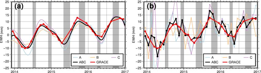
C. Lück et al.: Time-variable gravity fields from 37 months of kinematic Swarm orbits                                                    325

Table 1. Utilized orbit and star camera data.

                               Product                             Sampling                          Availability    Reference frame
          Kinematic orbits     ESA level 2 KIN                          10 s          1 Dec 2013 to (A: 15 Jul,           ITRF 2008
                               (van den IJssel et al., 2016)                          B: 15 Jul, C: 10 Jul) 2014
          Kinematic orbits     ESA level 2 KIN                            1s     (A: 15 Jul, B: 15 Jul, C: 10 Jul)        ITRF 2008
                               (van den IJssel et al., 2016)   (10 s is used)               2014 to 31 Dec 2016
          Star camera          ESA level 1b                               1s         1 Dec 2013 to 31 Dec 2016          ITRF 2008 to
                                                               (10 s is used)                                          satellite frame

Table 2. Background models used during the processing.

                   Background model                      Product                 Reference
                   Static field                          GOCO05c                 Pail et al. (2016)
                   Earth rotation                        IERS2010                Petit and Luzum (2010)
                   Moon, Sun and planets                 JPL DE421               Folkner et al. (2009)
                   Earth tide                            IERS2010                Petit and Luzum (2010)
                   Ocean tide                            EOT11a                  Savcenko and Bosch (2012)
                   Pole tide                             IERS2010                Petit and Luzum (2010)
                   Ocean pole tide                       Desai2004               Petit and Luzum (2010)
                   Atmospheric tides                     van Dam/Ray             van Dam and Ray (updated October 2010)
                   Atmosphere and ocean dealiasing       AOD1B RL05              Flechtner et al. (2015)
                   Permanent tidal deformation           included (zero tide)

NRLMSISE-00 model (Picone et al., 2002). NRLMSISE-                         of area averages for the total ocean as well as for comparison
00’s database includes total mass density from satellite ac-               to water storage change within various large terrestrial river
celerometers and POD, temperature from incoherent scatter                  basins (Sect. 3.3).
radar, and molecular oxygen number density collected under
different solar activity conditions. The model is driven by                3.1    Modeling of non-gravitational forces
the observed solar flux (F10.7 index) and geomagnetic index
(AP ). In Vielberg et al. (2018) we compare NRLMSISE-00                    While all three Swarm satellites carry accelerometers in-
to GRACE-derived thermospheric density and derive an em-                   tended to support POD and the study of the thermosphere,
pirical correction for this model; this has not yet been applied           these data have unfortunately turned out as severely affected
here.                                                                      by sudden bias changes (“steps”) and temperature-induced
                                                                           bias variations.
                                                                              Siemes et al. (2016) developed a method to clean and cal-
3   Methods                                                                ibrate the along-track acceleration of Swarm C. However,
                                                                           Swarm A and B (the former to a lesser extent than the lat-
In order to address our central question of to what extent                 ter), as well as the other C directions, are affected by seri-
will Swarm enable one to infer ocean mass change, we first                 ous issues and it is not clear whether these data can be used
compute time-variable gravity fields from kinematic orbits,                in gravity field applications. In the light of recent improve-
while considering different processing options. Then, ocean                ments of empirical thermosphere models (Vielberg et al.,
mass is derived from the computed Stokes coefficients (e.g.                2018) and seeing that we require all three components of
Chambers and Bonin, 2012), and results will be compared to                 non-conservative acceleration amodel for gravity recovery, we
the ITSG-GRACE solutions.                                                  decided instead to model them, using the well-known rela-
   In the following, we describe our modeling of the non-                  tion
conservative forces (Sect. 3.1), the processing method (in-
tegral equation approach with short arcs), and two options
for gravity field parameterization within the gravity recov-               amodel = adrag + aSRP + aERP .                                (1)
ery: (1) estimation of monthly fields and (2) estimation of
a CTAS model for each harmonic coefficient from the whole                  amodel is the sum of atmospheric drag adrag , solar radiation
mission lifetime in a single adjustment (Sect. 3.2). Finally,              pressure aSRP , and Earth radiation aERP . We will briefly sum-
results are compared to the ITSG-GRACE solution in terms                   marize our implementation below.

www.solid-earth.net/9/323/2018/                                                                              Solid Earth, 9, 323–339, 2018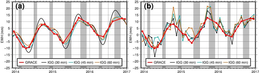
326 C. Lück et al.: Time-variable gravity fields from 37 months of kinematic Swarm orbits
3.1.1 Atmospheric drag Crd,i
j
+ crs,i cos 8inc,i n̂i + 1 − crs,i ŝ j . (5)
· 2
3
Atmospheric drag is commonly taken into account by evalu-
ating The satellite’s footprint is divided into M sections and R j
takes into account the effect of albedo and emission (we use
Aref 2 the Cloud and the Earth’s Radiant Energy System (CERES)
adrag = Cd ρv v̂r , (2)
2m r dataset EBAF-TOA Ed2.8 that provides monthly values;
where m is its mass, ρ the thermospheric density (here from (Loeb et al., 2009)). Different from the conventional imple-
NRLMSISE-00), vr the velocity of the satellite relative to the mentation (Knocke et al., 1988), we expanded these data into
atmosphere, and v̂r the normalized velocity vector relative to a low-degree spherical harmonic representation to account
the atmosphere. Aref is a reference area that cancels out in for longitudinal variations.
the computation of Cd (more precisely in the computation of
CD,i,j and CL,i,j , which will be introduced later), where the 3.2 Gravity field estimation
ratio of the area of each plate to Aref is taken into account. Cd
For gravity field estimation, we use the integral equation ap-
is evaluated as the sum over each plate i and each constituent
proach (Schneider, 1968; Reigber, 1969). Kinematic orbits
of the atmosphere j , as in
are partitioned into short arcs and each 3-D position r(τ ) be-
"
N X M
# tween the arc’s beginning and end (rA and rB ) can be ex-
X ρj
Cd = CD, i, j ûD + CL, i, j ûL, i · v̂r , (3) pressed as
i=1 j =1
ρ
Z1
where the contributions of drag CD, i, j and lift CL, i, j are 2
r(τ ) = rA (1 − τ ) + rB τ − T K(τ, τ 0 )f(τ 0 )dτ 0 , (6)
evaluated separately with their associated unit vectors ûD and
ûL,i . We follow Sentman et al. (1961) for further computa- 0
tions of CD, i, j and CL, i, j . with normalized time τ and the integral kernel, as in
3.1.2 Solar radiation pressure (
0 τ 0 (1 − τ ) for τ 0 ≤ τ
K(τ, τ ) = (7)
Solar radiation is absorbed or reflected at the satellite’s sur- τ (1 − τ 0 ) for τ 0 > τ.
face, leading to an acceleration (Sutton, 2008; Montenbruck
R1
and Gill, 2005), expressed as In other words, T 2 0 K(τ, τ 0 )f (τ 0 )dτ 0 in Eq. (6) represents
N
the offset of the current position from a straight line connect-
1AU2 RAi cos 8inc,i
ing rA and rB , caused by gravitational and non-gravitational
X
aSRP = −ν
i=1 r2 m forces f(τ 0 ). After discretization (sampling rate of kinematic
Crd,i
orbits is 1 s after July 2014), one can write the above as an ad-
· 2 + crs,i cos 8inc,i n̂i + 1 − crs,i ŝ . (4) justment problem with two groups of solved-for parameters
3
with the equation
Equation (4) accounts for SRP over each of the N plates of
the macro model. R is the solar flux constant valid at a dis- c20
tance of 1 astronomical unit (AU), Ai is the area of the ith c21
rA
plate, and crd,i and crs,i are the diffuse and specular reflec-
s21
y= rB and x = . (8)
tivity coefficients. 8inc,i denotes the angle between the Sun ..
accperArc
.
(unit vector ŝ) and the normal vector of each panel nˆi . The
snn
shadow function ν varies between 0 when the satellite is in accglobal
eclipse and 1 if it is fully illuminated. The term 1AU2 /r 2 ac-
counts for the eccentricity of the Earth’s orbit, with r being y contains all arc-related parameters, which can be elimi-
the varying Sun-satellite distance. nated from the normal equation system during the estima-
tion. These include start and end position of each arc and ad-
3.1.3 Earth radiation pressure ditional parameters such as accelerometer bias or scale fac-
tors. The gravity field parameters are then collected in x.
Radiation emitted from the Earth’s surface (ERP) is taken
For more details of the integral equation approach, see and
into account similar to solar radiation pressure with the equa-
Löcher (2010).
tion
In this study, we consider two different ways of parameter-
N X M
j
R j Ai cos 8inc,i izing the gravity field: (1) to be consistent with GRACE, we
X
aERP = − estimate monthly spherical harmonic coefficients complete
i=1 j =1
m to varying low degrees. (2) We use the CTAS solution: as we
Solid Earth, 9, 323–339, 2018 www.solid-earth.net/9/323/2018/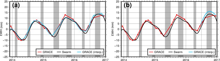
C. Lück et al.: Time-variable gravity fields from 37 months of kinematic Swarm orbits                                           327

Figure 1. Areas of investigation: ocean (OC), Amazon (AM), Mississippi (MI), Greenland (GR), Yangtze (YA), and Ganges (GA). The
boundaries are taken from the Food and Agriculture Organization of the United Nations (FAO).

aim at a long and stable time series, we additionally param-      model inconsistencies and should not be mixed up with in-
eterize a set of trends and semi-annual harmonic amplitudes       strument errors. We furthermore investigate the influence of
to the constant part for each Stokes coefficient in a single      different arc lengths, which affects the temporal acceleration
adjustment with the equation                                      parameterization, as well as the effect of spherical harmonic
                                                                  truncation.
cnm (t) = cnm + ċnm (t − t0 )

                   t − t0

                                           t − t0
                                                                 3.3   Ocean mass changes and river basin averages
      c1                         s1
  + cnm cos 2π                + cnm sin 2π
                     yr                      yr                   As was mentioned already, we choose different regions for

      c2           t −  t 0      s2        t −  t0                our investigation (see Fig. 1), but our focus is on the total
  + cnm cos 4π                + cnm sin 4π           ,
                     yr                      yr                   ocean in order to test the hypothesis that Swarm can bridge
snm (t) = s nm + ṡnm (t − t0 )                                   the GRACE ocean mass time series.
                                                                 For computing smoothed basin mass averages, let F (λ, 8)
      c1           t − t0        s1        t − t0
  + snm cos 2π                + snm sin 2π                        be the equivalent water height (EWH) derived from the
                     yr                      yr                   spherical harmonics (Wahr et al., 1998). The smoothed re-

      c2           t − t0        s2        t − t0                 gion average F OW , considering the smoothing kernel W
  + snm cos 4π                + snm sin 4π           .     (9)
                     yr                      yr                   (here a 500 km Gaussian filter) over the region O, can be
                                                                  expressed as
   We estimate the spherical harmonic coefficients from de-                 1
                                                                               Z
gree 2 onward. As described in Sect. 3.1, we derive non-          F OW =          OW (λ, θ )F dw.                         (10)
                                                                           OW
gravitational accelerations from models, which we then use
in the gravity field estimation as a proxy for accelerome-
ter measurements. Due to the presence of errors, e.g. those         The integral is effectively evaluated for the smoothed area
caused by uncertainties in the density model or errors in the     function OW (λ, θ ) as
macro model, the resulting non-gravitational accelerations                         n
                                                                                 ∞ X
might not always reflect the truth. To prevent these errors
                                                                                 X               W
                                                                  OW (λ, θ ) =                O nm Y nm (λ, θ )
from propagating into the gravity field estimates, it is com-                    n=0 m=−n
mon to introduce additional parameters. Here we co-estimate            1
                                                                           Z
an “accelerometer bias” per arc and per axis, either as a con-      =          W (λ, θ, λ0 , θ 0 )O(λ0 , θ 0 )dw 0 .            (11)
                                                                      4π
stant value or with an additional trend parameter. While we
found this usually sufficient, we also performed tests with an
additional global scaling factor per axis. Another possibility       Some postprocessing needs to be applied to the estimated
that is also evaluated in this paper is to co-estimate the bias   gravity fields, depending on the application. As we com-
globally. The influence of this “accelerometer parameteriza-      pare our results to the monthly GRACE solutions, we test
tion” will be evaluated in the course of this paper, yet one      replacing the c20 coefficient with those derived from satellite
needs to bear in mind that these parameters measure force         laser ranging (SLR) (Cheng et al., 2013). While replacing

www.solid-earth.net/9/323/2018/                                                                        Solid Earth, 9, 323–339, 2018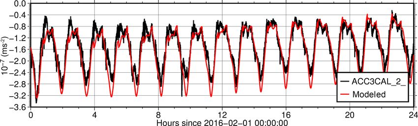
328                                        C. Lück et al.: Time-variable gravity fields from 37 months of kinematic Swarm orbits

Table 3. Parameterization for our monthly solutions and for our estimation of CTAS signal terms. All results are subject to a 500 km Gaussian
filter.

                       Arc length    Non-grav.      Bias                                       Scale    Maximum d/o
                       (min)         acc.
            Monthly    30            modeled        constant per arc (perArc0)                 none     estimated until 40, evaluated until 12
            CTAS       45            modeled        constant + trend per arc (perArc1)         none     static until 40 (evaluated until 12),
                                                                                                        time-variable until 12

Table 4. Parameterizations that have been tested in this study. This table should not be read row-wise. It lists all possible choices for each
heading. One solution can consist of any combination of the entries, for example, a monthly solution with an arc length of 60 min, modeled
non-gravitational accelerations, a constant global bias, no scaling factor, max. d/o estimated until 40, and evaluated until d/o 10.

       Arc length     Non-grav.     Bias                                 Scale                  Maximum d/o
       (min)          acc.
       30             not modeled   none                                 none       monthly:    estimated until 20/40, evaluated until 10/12/14
       45             modeled       constant per arc (perArc0)           global     CTAS:       static part until 20/40/60 (evaluated until 10/12/14),
       60                           constant + trend per arc (perArc1)                          time-variable part until 10/12/14
                                    constant global (global0)
                                    polyn. of deg. 4 global (global4)

c20 leads to a workflow more in line with GRACE, keeping
the Swarm-derived c20 would answer the question whether
Swarm alone is able to measure mass change relative to a ref-
erence (here GOCO05c). In the next step, we add all de-
gree 1 coefficients to correct for geocenter motion (Swen-
son et al., 2008), which cannot be detected with the current
GRACE and Swarm processing. We apply a correction for
glacial isostatic adjustment following A et al. (2013), but as
long as we apply the same correction to GRACE, the com-
parison between Swarm and GRACE will be independent of
this choice. We employed an ocean mask that includes the
Arctic ocean and does not have a coastal buffer zone.

                                                                                  Figure 2. Ocean mass from ITSG-Grace2016 and Swarm. GRACE
4     Results                                                                     data gaps are highlighted in gray.
If not stated differently, we used the parameterization in Ta-
ble 3 for monthly ocean mass or ocean mass from a direct
estimation of CTAS signal terms. We chose these parameter-                        IGG time-variable gravity field was computed with an arc
izations because they represent our best monthly solution (as                     length of 30 min, modeled non-gravitational accelerations,
will be seen in Fig. 11) and the best CTAS solution up to de-                     and a constant bias per arc and direction being co-estimated,
gree and order (d/o) 12 (see Fig. 10). The choice of the same                     which leads to our best solution. All Swarm time series show
degree allows a comparison of the results. Our test studies                       a behavior similar to the GRACE solution, but they appear
include all possible combinations of the parameterizations                        overall noisier, as can be seen from the variances in Table 6.
shown in Table 4, which leads to more than 500 configura-                         The quality of all solutions improves after the global navi-
tions.                                                                            gation satellite system (GNSS) receiver update in July 2014.
                                                                                  The impact of tracking loop updates on gravity field recovery
4.1    Ocean mass from GRACE and Swarm                                            is discussed in Dahle et al. (2017). It is furthermore interest-
                                                                                  ing to compute the RMSE of all solutions when we assume
Figure 2 shows monthly ocean mass change in mm EWH de-                            the GRACE solution to be the truth (first row of Table 6).
rived from GRACE as a reference and from different Swarm                          The ASU time series has the lowest RMSE, with 2.8 mm; it
time-variable gravity (TVG) solutions from AIUB, ASU,                             is closest to GRACE. The IGG solution has the second low-
IfG and the Institute of Geodesy and Geoinformation (IGG)                         est RMSE, with 4.0 mm. To assess the spread between the
in Bonn (processing details can be found in Table 5). The                         different Swarm solutions, we compute the RMSE for each

Solid Earth, 9, 323–339, 2018                                                                                    www.solid-earth.net/9/323/2018/
C. Lück et al.: Time-variable gravity fields from 37 months of kinematic Swarm orbits 329
Table 5. Comparison of Swarm solutions from different institutes. Orbit product, computing method, and maximum d/o are provided.
AIUB ASU IGG IfG
Orbit AIUB (screened version) ITSG ESA IfG
Approach Celestial mechanics approach Acceleration approach Short-arc approach Short-arc approach
max d/o 70 40 40 60
Table 6. Comparison of the variance (mm) of the individual ocean
mass time series (main diagonal) and the RMSE (mm) between two
solutions (off-diagonal). The results are based on the time series of
Fig. 2.
GRACE AIUB ASU IGG IfG
GRACE 6.6 5.1 2.8 4.0 5.2
AIUB 7.4 4.5 4.3 5.4
ASU 7.3 4.2 4.1
IGG 7.5 5.6
IfG 8.5
combination (off-diagonal of Table 6) which is of the same
magnitude as the RMSEs of GRACE and Swarm. Figure 3. Degree variances for GRACE and Swarm (solution for
An important issue in extending the ocean mass time series May 2016). Formal errors as well as the difference degree variance
is the accuracy of the trend. Table 7 shows the trends as well (GRACE minus Swarm) are shown with dotted lines.
as the amplitude and phase of the Swarm solutions. The trend
of the IGG solution (3.3 mm yr−1 ) is the closest to GRACE
(3.5 mm yr−1 ). While the trend over three years itself cannot
be considered as representative for the GRACE era due to
interannual variability of barotropic modes, this suggests that Eq. 9) until d/o 20, 40, or 60, while the time-variable part
Swarm data could be used to bridge a gap between GRACE is estimated until d/o 10, 12, or 14.
and GRACE-FO.
Figure 3 shows the degree variances and the difference de-
gree variances of GRACE and our IGG solution for May 4.2 Effect of modeling of non-gravitational forces
2016 with respect to our reference field GOCO05c. Obvi-
ously, the higher the degree, the higher is the discrepancy be-
tween GRACE and Swarm. The difference (dotted gray line) Figure 4 compares modeled non-gravitational accelerations
indicates that for this particular month Swarm is only reli- (see Sect. 3.1) to the ACC3CAL_2_ product from Siemes
able for degrees up to about 10, which is due to the much et al. (2016), who removed sudden bias changes from
lower precision of the GPS data compared to the GRACE the accelerometer measurements and corrected the low-
inter-satellite K-band ranging. Since the formal errors (dotted frequencies with POD-derived non-gravitational accelera-
black line) are not calibrated, they are too optimistic and al- tions. Both time series are very close together, which sup-
ways lower than the difference between GRACE and Swarm. ports our use of the modeled non-gravitational accelerations
This will be addressed in the future by including realistic co- for gravity field estimation. Small systematic deviations can
variance information of the kinematic orbits. As Fig. 3 only be compensated for by co-estimating additional bias or scale
shows the degree variances for one particular month, we in- parameters.
vestigate different maximum degrees in the following (see Modeling non-gravitational accelerations from the Swarm
Table 4). We evaluate our monthly fields until d/o 10, 12 satellites within TVG recovery provides an ocean mass time
or 14. Even though higher degrees do not contribute a rea- series significantly closer to the one from GRACE (see
sonable time-variable signal, we estimate the monthly fields Fig. 5), and it also improves the trend estimate as can be seen
until d/o 20 or 40, because high degrees can absorb errors in Table 8. This means that errors caused by neglecting non-
that would otherwise propagate in the lower degrees. For our gravitational accelerations would propagate in the spherical
CTAS solution, we estimate a static part (cnm and s nm in harmonic coefficients.
www.solid-earth.net/9/323/2018/ Solid Earth, 9, 323–339, 2018330 C. Lück et al.: Time-variable gravity fields from 37 months of kinematic Swarm orbits
Table 7. Comparison of Swarm solutions from different institutes measuring trend, amplitude, and phase. The values in parentheses indicate
the results for the exact same months that are available for GRACE, while the values without parentheses are computed from the whole
Swarm time series. The results are based on the time series of Fig. 2.
GRACE AIUB ASU IGG IfG
Trend (mm yr−1 ) 3.5 2.1 (3.2) 4.2 (4.6) 3.3 (4.3) 2.4 (3.2)
Amplitude (annual) (mm) 7.9 7.4 (7.6) 6.9 (8.1) 6.8 (7.8) 9.0 (10.1)
Amplitude (semiannual) (mm) 1.1 2.9 (4.5) 0.5 (0.8) 2.3 (0.8) 1.2 (1.9)
Phase (annual) (days) −12.0 −12.4 (−11.7) −12.1 (−12.4) −12.8 (−12.4) −12.6 (−12.2)
Phase (semiannual) (days) 6.6 13.4 (13.2) 13.7 (12.4) 7.8 (12.4) −9.9 (−12.2)
Figure 4. Along-track acceleration of Swarm C. The black curve shows the ACC3CAL_2_ product from Siemes et al. (2016), while the red
curve shows our modeled non-gravitational accelerations without applying any bias or scale factors.
Figure 5. Effect of modeling of non-gravitational forces on ocean Figure 6. Ocean mass from GRACE and Swarm. The monthly so-
mass computation. IGG (mod.) is the monthly solution described lution is shown in black while the CTAS solution is shown in blue.
in Table 3. The only difference in IGG (not mod.) is that non- The parameterizations for the two solutions can be found in Table 3.
gravitational accelerations were not modeled, but a constant value
per arc was still co-estimated.
leads to solutions which are much closer to GRACE. The
reason for this is that the estimation of CTAS terms from the
4.3 Effect of gravity field parameterization whole Swarm period (December 2013 to December 2016) is
more stable than estimating a set of spherical harmonic coef-
Figure 6 shows (1) monthly Swarm solutions compared to ficients for each month. To our knowledge, this has not been
(2) ocean mass derived with a CTAS signal for each spheri- investigated for Swarm, prior to this study.
cal harmonic coefficient. Obviously, the second approach fits
much better to the GRACE time series, depicted in red: the 4.4 Effect of different arc lengths
RMSE decreases from 4.0 mm for (1) to only 1.7 mm for (2).
Furthermore, we find a trend estimate of 3.5 mm yr−1 , which We investigated the effect of different arc lengths of 30, 45,
is surprisingly close to GRACE (see Table 8). In other words, and 60 min on ocean mass estimates (see Fig. 7). The remain-
directly parameterizing CTAS terms for each harmonic co- ing parameters have been chosen according to our best re-
efficient, instead of computing the usual monthly solutions, sults. For the CTAS approach, the solution with 30 min dif-
Solid Earth, 9, 323–339, 2018 www.solid-earth.net/9/323/2018/C. Lück et al.: Time-variable gravity fields from 37 months of kinematic Swarm orbits 331
Table 8. Comparison of different IGG Swarm solutions. IGG: best monthly IGG solution. IGG (not mod.): same parameterization as IGG,
but non-gravitational accelerations are not modeled. IGG (CTAS): IGG solution with an estimated constant, trend, annual and semiannual
signal per spherical harmonic coefficient. The values in parentheses indicate the results for the exact same months that are available for
GRACE, while the values without parentheses are computed from the whole Swarm time series.
GRACE IGG IGG (not mod.) IGG (CTAS)
Trend [mm yr−1 ] 3.5 3.3 (4.3) 4.0 (4.4) 3.5 (3.5)
Amplitude (annual) [mm] 7.9 6.8 (7.8) 8.3 (9.3) 7.4 (7.3)
Amplitude (semiannual) [mm] 1.1 2.3 (3.2) 2.6 (3.3) 1.9 (1.9)
Phase (annual) [days] −12.0 −12.8 (−13.2) −13.1 (−12.9) −10.6 (−10.6)
Phase (semiannual) [days] 6.6 7.8 (9.4) 3.5 (4.9) 8.7 (8.7)
Figure 7. Effect of varying the arc length. (a) CTAS solution. (b) Monthly solutions.
Figure 8. Effect of co-estimating bias and scale factors for the non-gravitational accelerations. The numbers indicate the degree of the
polynomial. (a) CTAS solutions. (b) Monthly solutions.
fers most from GRACE and the other two solutions, while and scale factors” (see Sect. 3.2). For Figs. 8a and b we find
45 min provide the lowest RMSE (1.7 mm) and the best that a global scaling factor per axis only has a minor influ-
trend estimate (3.5 mm yr−1 ). When considering monthly so- ence.
lutions, 30 min provide the best result (RMSE: 4.0 mm and For the CTAS solutions, parameterizing the bias as a linear
trend: 3.3 mm yr−1 ). function leads to a smaller RMSE with respect to the GRACE
solution than a constant value per axis or not estimating it at
4.5 Effect of the parameterization of non-gravitational all. The reason for this might be the large number of obser-
forces vations (10 s sampling for 37 months) compared to the low
number of parameters. The additional parameters per arc give
In addition to modeling the non-gravitational forces, which room for improving not only the modeled non-gravitational
are introduced in the gravity estimation process as ac- accelerations but also the gravity field parameters. Looking
celerometer data, we carried out several tests, as listed in Ta- at monthly solutions, we find that a constant bias per axis
ble 4, concerning the co-estimation of “accelerometer bias
www.solid-earth.net/9/323/2018/ Solid Earth, 9, 323–339, 2018332 C. Lück et al.: Time-variable gravity fields from 37 months of kinematic Swarm orbits
Figure 9. Influence of individual satellites on the combined solution. (a) CTAS solutions. (b) Monthly solutions.
has a smaller RMSE with respect to GRACE than a linear tio (SNR), expressed as
function or not estimating a bias.
For (a) and (b) we also introduced the bias as a constant
VAR F OW ,GRACE (t)
value or a polynomial of degree 4 for the whole time span SNR = . (12)
of either 37 months (a) or 1 month (b). The two solutions do RMSE F OW ,Swarm (t)
not differ much, but they are of a minor quality compared to
other solutions. Figure 10 shows the 100 best CTAS solutions (considering
SNR for the ocean), while Fig. 11 shows an equal number
4.6 Contribution of Swarm satellites A, B, and C of the best monthly solutions. To get an idea of the signals
in the different basins, Fig. 12 shows the EWH derived from
GRACE.
In this study, we combine the information from the three In general, the quality of the time series of the EWH de-
spacecrafts by simply accumulating the normal equations. rived from kinematic orbits of Swarm will be affected by
For reasons of interpretation and validation, it makes sense to (1) the basin size (see Fig. 1) and (2) the signal strength (see
also investigate the single-satellite solutions. Figure 9 com- Fig. 12). As expected, the ratio of VAR / RMSE is highest for
pares ocean mass change derived from the individual solu- the ocean, followed by the Amazon basin, which means that
tions, from the combined solution, and from GRACE for these results are the most reliable. The reason for the good
(a) the CTAS solutions and (b) the monthly solutions. It is performance of Swarm is the large basin size for the ocean
expected that Swarm A and Swarm C provide similar solu- and the large signal combined with a large area for the Ama-
tions as they fly side by side. This is the case for the CTAS zon basin. For the Greenland and Ganges mass estimates
solutions, but it is not always true for the monthly solutions. there are some CTAS solutions with VAR / RMSE > 1 and
One possible explanation is that the receivers have different in general, the time series of these two basins have a higher
settings, which were activated at different times (van den IJs- VAR / RMSE than those for the Mississippi and Yangtze
sel et al., 2016; Dahle et al., 2017). basins, both for the CTAS and the monthly solutions. Consid-
ering monthly solutions, modeling non-gravitational acceler-
ations provides better results than not modeling them. This
4.7 River basin mass estimates
can be seen in Fig. 11, where only very few solutions with
no modeled non-gravitational accelerations are present. The
Even though we concentrated on ocean mass in this study, we best CTAS solutions for the ocean also have modeled non-
also derived river basin mass estimates to validate our TVG gravitational accelerations, whereas for solutions 13 to 15
results in land regions. We investigated the same parameter- only empirical accelerations were co-estimated. These have
izations that we used to derive ocean mass changes (see Ta- been obtained with a higher VAR / RMSE for the Amazon,
ble 4). To assess the solutions with regard to their quality, we Mississippi, Greenland, and Ganges basins. The estimation
compared our results to those derived from the GRACE mis- of a bias is mandatory as both the best CTAS and monthly
sion. We decided to not only compute the RMSE, but also solutions always have a bias co-estimated. The best monthly
to compute the ratio of the variance (VAR) of the GRACE solution was computed until d/o 40 and both GRACE and
time series to the RMSE. By using this method we can also Swarm were evaluated until d/o 12. This is followed by solu-
compare the quality of the solutions in the different areas. tions that were evaluated until d/o 10. The time-variable part
The RMSE will be calculated with respect to the available of the best CTAS solution is even estimated and evaluated
GRACE data (27 out of 37 months from December 2013 to until d/o 14. In general, the results confirm what has been
December 2016). This will give a kind of signal-to-noise ra- evaluated in Sects. 4.2 to 4.5.
Solid Earth, 9, 323–339, 2018 www.solid-earth.net/9/323/2018/C. Lück et al.: Time-variable gravity fields from 37 months of kinematic Swarm orbits 333 Figure 10. Evaluation of methods (CTAS solutions). www.solid-earth.net/9/323/2018/ Solid Earth, 9, 323–339, 2018
334                                 C. Lück et al.: Time-variable gravity fields from 37 months of kinematic Swarm orbits

Figure 11. Evaluation of methods (monthly solutions).

Solid Earth, 9, 323–339, 2018                                                            www.solid-earth.net/9/323/2018/
C. Lück et al.: Time-variable gravity fields from 37 months of kinematic Swarm orbits                                                335

Table 9. Mean RMSE (mm) of the gap-filler methods with respect to existing GRACE data. The columns indicate the number of missing
months. The percentage of Swarm (CTAS) solutions with a lower RMSE than GRACE (interpolated) solutions is indicated in parentheses.
To derive the value in parentheses, we counted the number of CTAS solutions with a lower RMSE than GRACE (interpolated) and computed
the relation to the absolute number of CTAS solutions. The number of investigated solutions decreases from left to right, as the time span
becomes longer.

                                                         1              3              6            12              18
                    GRACE (interpolated)               0.9             1.1            1.1           1.2             1.8
                    Swarm (CTAS)              1.4 (13.5 %)    1.5 (17.1 %)    1.6 (6.3 %)   1.6 (3.8 %)    1.6 (80.0 %)
                    Swarm (monthly)                    3.3             3.7            3.8           3.9             3.8

                                                                           In case of a longer gap between GRACE and GRACE-
                                                                        FO, ocean mass estimates from Swarm will become more
                                                                        important than considering missing monthly solutions. Fig-
                                                                        ure 13b shows what would happen if the last 6 months of
                                                                        GRACE were missing. We use the same procedure as before
                                                                        by estimating a harmonic signal (CTAS) from the remain-
                                                                        ing GRACE data. This leads to the blue curve, which is fur-
                                                                        ther offset from GRACE than our Swarm solution. Over 3
                                                                        years, this would also lead to a degradation of the trend es-
                                                                        timate (GRACE and Swarm: 3.5 mm yr−1 and interpolated
                                                                        GRACE: 4.0 mm yr−1 ), indicating that Swarm is useful to
                                                                        bridge longer gaps, which will be investigated in the follow-
                                                                        ing paragraph.
                                                                           We simulated all possible gaps with a duration between
Figure 12. EWH derived from GRACE (d/o 12, 500 km Gaussian              1 month and 18 months in the time series from December
filter) for different regions. The time series have been reduced by     2013 to December 2017 and tested all gap-filling methods
their mean values for reasons of comparison.                            (interpolating GRACE, using monthly Swarm solutions, and
                                                                        using CTAS Swarm solutions). For example, when we as-
                                                                        sumed a gap of three months, we investigated gaps from De-
                                                                        cember 2013 to February 2014 until October 2016 to Decem-
4.8   Bridging a possible gap with Swarm                                ber 2016, which created 35 possibilities. The mean RMSE,
                                                                        with respect to the real GRACE data, is shown in Table 9. It
As GRACE has met the end of its lifetime, we make efforts               is obviously better to use our CTAS solution to fill gaps in-
here to close the gap until GRACE-FO provides data. We                  stead of using monthly solutions. However, for a gap of three
study as well the possibility to fill monthly gaps, which are           months, we get a mean RMSE of 1.1 mm for interpolating ex-
usually bridged by interpolating the previous and subsequent            isting GRACE solutions compared to 1.5 mm for the CTAS
monthly solutions. To find out whether Swarm TVG should                 solution, which indicates that in most cases of a three-month
be preferred to interpolating GRACE data, we assume that                gap, interpolating the remaining GRACE solutions is closer
existing monthly solutions are missing, such that we are still          to GRACE than using the Swarm solutions. For a prolonged
able to compare to the actual solutions. In Fig. 13a we as-             gap of 18 months, our Swarm solution would, however, be
sumed each individual monthly GRACE solution to be miss-                closer to GRACE in 80 % of all cases.
ing at one time. We then estimated a harmonic time series
consisting of CTAS terms from all solutions except for the              4.9   Is it possible to detect La Niña events with Swarm?
one that is considered to be missing. After having carried out
the regression for each month, this leads to the blue curve.            With the Swarm accuracy as discussed in Table 6, the next
When comparing the interpolated GRACE time series to the                logical question would be to ask what kind of sea level sig-
Swarm solution, we find that they are both very close to                nal could be detected with Swarm. During the time span in-
the real GRACE solution, which offers two possibilities for             vestigated here (December 2013 to December 2016), ocean
bridging monthly gaps in the GRACE time series. For most                mass evolves rather regularly, i.e. without apparent interan-
months, the interpolated GRACE time series is closer to the             nual variation. Therefore, we decided to look into data from
real GRACE solution, which means that it is more reliable to            the past.
close monthly gaps by interpolating than by using the Swarm                Boening et al. (2012) and Fasullo et al. (2013) showed that
solutions.                                                              the 2010/11 La Niña event led to a 5 mm drop in global mean

www.solid-earth.net/9/323/2018/                                                                           Solid Earth, 9, 323–339, 2018
336 C. Lück et al.: Time-variable gravity fields from 37 months of kinematic Swarm orbits
Figure 13. Bridging gaps with Swarm. Our IGG Swarm solution (black) is compared to the monthly GRACE solutions (red) as well as
to interpolated values when we assume a part of the GRACE time series to be missing. (a) Each month is assumed to be missing and is
interpolated from all other months. (b) The last 6 months are assumed to be missing and are interpolated from all other months.
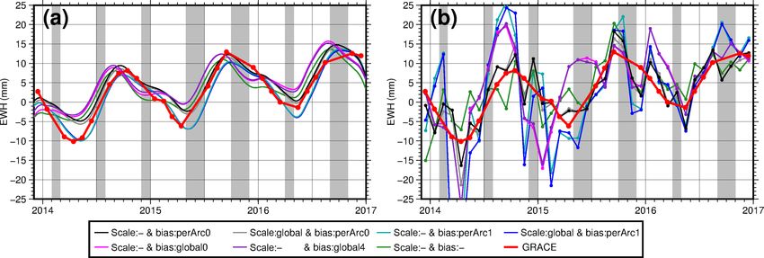
Figure 14. Time series of ocean mass (red). A variance of 4.0 mm is shaded in pink to simulate the uncertainty of Swarm mass estimates.
A moving average filter of 1 year is applied (black) and the resulting standard deviation is shown in gray. (a) Simulation of ocean mass (red)
from Wenzel and Schröter (2007); 1993–2004. (b) Ocean mass from GRACE; 2004–2014. (c) Ocean mass from Swarm; 2014–2016. There
is an offset between offset between panel (a) and panels (b) and (c) because of different mean fields.
sea level (GMSL). This has been derived from satellite al- tify the drop between 1998 and 2000 standing out against the
timetry as well as from a combination of GRACE and Argo noise floor. To recap, strong La Niña events such as they oc-
data. As most of the anomaly has been shown to be caused by curred in the past could be observed with Swarm, which will
mass changes, it is reasonable to ask whether we would have be of special importance in case of a prolonged gap between
been able to observe the drop in ocean mass with Swarm (or GRACE and GRACE-FO.
to observe a similar event in the future). A simple computa- So far, ocean mass has been shown without adding back
tion shows that with an RMSE of 4.0 mm for monthly Swarm the GAD product from the German Research Centre for Geo-
solutions,√we would be able to detect a 6-month drop of sciences (Flechtner et al., 2015) to our previous time series
4.0 mm/ 6 = 1.6 mm. As the 2010/11 drop was both larger since our focus is on comparing estimates and the GAD prod-
and lasted longer, we conclude that we should have been able uct has a trend of zero for the ocean basin. Here, for better
to detect La Niña events with Swarm, therefore making it interpretation, we show ocean mass from GRACE from 2004
likely to be able to do so in the future. to 2014 (Fig. 14b) and ocean mass from Swarm from 2014
We have conducted another simulation experiment with to 2016 (Fig. 14c) with the GAD product added back.
simulated ocean mass data from 1993 to 2004 taken from
Wenzel and Schröter (2007) (see Fig. 14a). Using the Wen-
zel and Schröter time series as a basis here, we then gen- 5 Conclusions
erate 1000 simulated Swarm time series by adding white
noise with a variance of 4.0 mm (pink area). When compar- Swarm-derived ocean mass estimates show the same behav-
ing the filtered (moving average of 1 year) time series shown ior as those from GRACE, but they appear overall nois-
as black line with standard deviation of 1.2 mm derived from ier, as expected. IGG monthly solutions have an RMSE of
the simulated Swarm time series (gray), we can clearly iden- 4.0 mm with respect to GRACE, which is comparable or
better than the solutions from other institutions that we in-
Solid Earth, 9, 323–339, 2018 www.solid-earth.net/9/323/2018/C. Lück et al.: Time-variable gravity fields from 37 months of kinematic Swarm orbits 337
vestigated (AIUB, ASU, and IfG). Over the Swarm period Data availability. – The GRACE spherical harmonic coeffi-
we find a mass trend of 3.3 mm yr−1 , which is close to that cients that were used for comparison can be found at ftp://ftp.
from GRACE (3.5 mm yr−1 ). The spread between the differ- tugraz.at/outgoing/ITSG/GRACE/ITSG-Grace2016/monthly/.
ent Swarm solutions is of the same order of magnitude as the – The Swarm spherical harmonic coefficients from IfG Graz
RMSE of Swarm with respect to GRACE. The degree vari- can be found at http://ftp.tugraz.at/outgoing/ITSG/tvgogo/
ances for monthly solutions suggest that the TVG fields are gravityFieldModels/Swarm/.
only reliable up to about degrees 10–12. – The Swarm spherical harmonic coefficients from ASU Prague
In a second approach we estimated CTAS terms for each can be found at http://www.asu.cas.cz/~bezdek/vyzkum/
spherical harmonic coefficient and for the whole period geopotencial/index.php.
of time under study (December 2013 to December 2017).
– The employed CERES data can be found at http://ceres.larc.
We find that this significantly improves the agreement with nasa.gov/order_data.php.
GRACE regarding ocean mass trend estimates; here we ob-
tain an RMSE of 1.7 mm and the same trend as derived
from GRACE. We investigated different parameterizations Competing interests. The authors declare that they have no conflict
and found that an arc length of 30 min provides the best re- of interest.
sults for monthly solutions, while 45 min is the best option
for the CTAS solutions. Furthermore, co-estimating an “ac-
celerometer bias” proved to be important. A constant bias Special issue statement. This article is part of the special issue
per arc and axis leads to the lowest RMSE with respect to “Dynamics and interaction of processes in the Earth and its space
GRACE for monthly solutions and an additional trend pa- environment: the perspective from low Earth orbiting satellites and
rameter is needed for the CTAS approach. beyond”. It does not belong to a conference.
We validated TVG results by computing river basin mass
estimates and comparing them to GRACE. We found that the
VAR / RMSE ratio, which can be considered as a signal-to- Acknowledgements. This study is supported by the Priority Pro-
noise ratio, is highest for the ocean, followed by the Ama- gram 1788 “Dynamic Earth” of the German Research Founda-
zon basin. Some of the Greenland and Ganges solutions also tion (DFG) – FKZ: KU 1207/21-1. The authors are grateful for
the Swarm macro model as well as the calibrated accelerometer
show a SNR larger than one, while Swarm-derived surface
data from Christian Siemes (ESA). We also would like to thank
mass change over the Yangtze and Mississippi is worse. Christoph Dahle for sending us the Swarm gravity fields from AIUB
We tested three different methods for filling the gap that (Bern).
now will occur between GRACE and GRACE-FO, as well We appreciate the work of Jose van den IJssel, whose kinematic
as for reconstructing missing single months in the GRACE orbits are available on the ESA FTP server. Thanks to Torsten
time series: (1) interpolating existing monthly GRACE so- Mayer-Gürr and his colleagues from IfG Graz and Aleš Bezděk
lutions, (2) using monthly Swarm solutions, (3) using the (ASU Prague) for providing their gravity solutions online.
CTAS Swarm solution. As expected, (3) provides better re-
sults than (2) and whether (1) or (3) is better depends on the Edited by: Simon McClusky
length of the gap and on the presence of episodic events and Reviewed by: three anonymous referees
interannual variability. In the (short) Swarm period where
ocean mass displayed little variability beyond the annual cy-
cle, we found that for reconstructing either single months or
References
three-month periods (1) may work slightly better than (3),
whereas in case of a long 18-month gap, (3) should be pre- A, G., Wahr, J., and Zhong, S.: Computations of the vis-
ferred. coelastic response of a 3-D compressible Earth to sur-
We showed that La Niña events like those from 2010– face loading: an application to Glacial Isostatic Adjustment
2011 and 1998–2000 could have been identified with Swarm, in Antarctica and Canada, Geophys. J. Int., 192, 557–572,
which is of special importance for the future after the termi- https://doi.org/10.1093/gji/ggs030, 2013.
nation of the GRACE mission. Bezděk, A., Sebera, J., Teixeira da Encarnação, J., and
In future work, we will concentrate on improving our Klokočník, J.: Time-variable gravity fields derived from
ocean mass estimates from Swarm by allowing the trend to GPS tracking of Swarm, Geophys. J. Int., 205, 1665–1669,
https://doi.org/10.1093/gji/ggw094, 2016.
change over time as shown, for example, in Didova et al.
Boening, C., Willis, J. K., Landerer, F. W., Nerem, R. S., and Fa-
(2016). Furthermore, we work towards ingesting our Swarm
sullo, J.: The 2011 La Niña: So strong, the oceans fell, Geophys.
solutions at the normal equation level into the fingerprint Res. Lett., 39, l19602, https://doi.org/10.1029/2012GL053055,
inversion of Rietbroek et al. (2016), to improve existing 2012.
sea level budget results and to partition altimetric sea level Cazenave, A. and Llovel, W.: Contemporary Sea Level Rise, Annu.
changes into its different components, even for those periods Rev. Mar. Sci., 2, 145–173, https://doi.org/10.1146/annurev-
where we do not have GRACE data. marine-120308-081105, 2010.
www.solid-earth.net/9/323/2018/ Solid Earth, 9, 323–339, 2018338 C. Lück et al.: Time-variable gravity fields from 37 months of kinematic Swarm orbits Chambers, D. P. and Bonin, J. A.: Evaluation of Release-05 GRACE of the AIAA/AAS, Astrodynamics Conference, 15–17 August time-variable gravity coefficients over the ocean, Ocean Sci., 8, 1988, Minneapolis, USA, 577–586, 1988. 859–868, https://doi.org/10.5194/os-8-859-2012, 2012. Llovel, W., K. Willis, J., Landerer, F., and Fukumori, I.: Deep- Cheng, M., Tapley, B. D., and Ries, J. C.: Deceleration in the ocean contribution to sea level and energy budget not de- Earth’s oblateness, J. Geophys. Res.-Sol. Ea., 118, 740–747, tectable over the past decade, Nat. Clim. Change, 4, 1031–1035, https://doi.org/10.1002/jgrb.50058, 2013. https://doi.org/10.1038/nclimate2387, 2014. Dahle, C., Flechtner, F., Gruber, C., König, D., König, R., Micha- Löcher, A.: Möglichkeiten der Nutzung kinematischer Satelliten- lak, G., and Neumayer, K.-H.: GFZ GRACE Level-2 Process- bahnen zur Bestimmung des Gravitationsfeldes der Erde, Disser- ing Standards Document for Level-2 Product Release 0005, tation, Universität Bonn, Bonn, Germany, 2010. Tech. rep., Deutsches GeoForschungsZentrum, Potsdam, Ger- Loeb, N. G., Wielicki, B. A., Doelling, D. R., Smith, G. L., many, https://doi.org/10.2312/GFZ.b103-12020, 2012. Keyes, D. F., Kato, S., Manalo-Smith, N., and Wong, T.: Dahle, C., Arnold, D., and Jäggi, A.: Impact of track- Toward Optimal Closure of the Earth’s Top-of- ing loop settings of the Swarm GPS receiver on grav- Atmosphere Radiation Budget, J. Climate, 22, 748–766, ity field recovery, Adv. Space Res., 59, 2843–2854, https://doi.org/10.1175/2008JCLI2637.1, 2009. https://doi.org/10.1016/j.asr.2017.03.003, 2017. Lombard, A., Garcia-Sanoguera, D., Ramillien, G., Cazenave, A., Didova, O., Gunter, B., Riva, R., Klees, R., and Roese- Biancale, R., Lemoine, J.-M., Flechtner, F., Schmidt, R., and Koerner, L.: An approach for estimating time-variable rates Ishii, M.: Estimation of steric sea level variations from combined from geodetic time series, J. Geodesy, 90, 1207–1221, GRACE and Jason-1 data, Earth Planet. Sc. Lett., 254, 194–202, https://doi.org/10.1007/s00190-016-0918-5, 2016. https://doi.org/10.1016/j.epsl.2006.11.035, 2007. Fasullo, J. T., Boening, C., Landerer, F. W., and Nerem, R. S.: Mayer-Gürr, T.: Gravitationsfeldbestimmung aus der Analyse Australia’s unique influence on global sea level in kurzer Bahnbögen am Beispiel der Satellitenmissionen CHAMP 2010–2011, Geophys. Res. Lett., 40, 4368–4373, und GRACE, Dissertation, Universität Bonn, Bonn, Germany, https://doi.org/10.1002/grl.50834, 2013. 2006. Flechtner, F.,Dobslaw, H., and Fagiolini, E.: GRACE 327-750 (GR- Mayer-Gürr, T., Behzadpour, S., Ellmer, K., Kvas, A., Klinger, B., GFZ-AOD-0001). AOD1B Product Description Document for and Zehentner, N.: ITSG-Grace2016 – Monthly and Daily Product Release 05, Tech. rep., GFZ, Potsdam, Germany, 2015. Gravity Field Solutions from GRACE, GFZ Data Services, Folkner, W. M., Williams, J. G., and Boggs, D. H.: The Planetary https://doi.org/10.5880/icgem.2016.007, 2016. and Lunar Ephemeris DE 421, Tech. rep., Jet Propulsion Labo- Montenbruck, O. and Gill, E.: Satellite Orbits: Models, Methods, ratory, Pasadena, California, USA, 2009. Applications, Springer, Berlin Heidelberg, Germany, 2005. Friis-Christensen, E., Lühr, H., Knudsen, D., and Haag- Nicholls, R. J. and Cazenave, A.: Sea-Level Rise and Its mans, R.: Swarm – An Earth Observation Mission in- Impact on Coastal Zones, Science, 328, 1517–1520, vestigating Geospace, Adv. Space Res., 41, 210–216, https://doi.org/10.1126/science.1185782, 2010. https://doi.org/10.1016/j.asr.2006.10.008, 2008. Olsen, N., Friis-Christensen, E., Floberghagen, R., Alken, P., Beg- Gerlach, C. and Visser, P.: Swarm and gravity: Possibilities and ex- gan, C. D., Chulliat, A., Doornbos, E., da Encarnação, J. T., pectations for gravity field recovery, in: Proceedings of the First Hamilton, B., Hulot, G., van den IJssel, J., Kuvshinov, A., Swarm International Science Meeting, 3–5 May 2006, Nantes, Lesur, V., Lühr, H., Macmillan, S., Maus, S., Noja, M., France, edited by: Danesy, D., Nantes, 2006. Olsen, P. E. H., Park, J., Plank, G., Püthe, C., Rauberg, J., Gregory, J. M., White, N. J., Church, J. A., Bierkens, M. F. P., Ritter, P., Rother, M., Sabaka, T. J., Schachtschneider, R., Box, J. E., van den Broeke, M. R., Cogley, J. G., Fettweis, X., Sirol, O., Stolle, C., Thébault, E., Thomson, A. W. P., Tøffner- Hanna, E., Huybrechts, P., Konikow, L. F., Leclercq, P. W., Clausen, L., Velímský, J., Vigneron, P., and Visser, P. N.: The Marzeion, B., Oerlemans, J., Tamisiea, M. E., Wada, Y., Swarm Satellite Constellation Application and Research Facility Wake, L. M., and van de Wal, R. S. W.: Twentieth- (SCARF) and Swarm data products, Earth Planets Space, 65, 1, Century Global-Mean Sea Level Rise: Is the Whole Greater https://doi.org/10.5047/eps.2013.07.001, 2013. than the Sum of the Parts?, J. Climate, 26, 4476–4499, Pail, R., Gruber, T., Fecher, T., and GOCO Project Team: The https://doi.org/10.1175/JCLI-D-12-00319.1, 2013. Combined Gravity Model GOCO05c, GFZ Data Services, Gunter, B., Encarnação, J., and Ditmar, P.: The use of satellite con- https://doi.org/10.5880/icgem.2016.003, 2016. stellations and formations for future satellite gravity missions, Petit, G. and Luzum, B.: IERS Conventions (2010) (IERS Technical Adv. Astronaut. Sci., 134, 1357–1368, 2009. Note No. 36), Tech. rep., International Earth Rotation and Refer- Jäggi, A., Beutler, G., Prange, L., Dach, R., and Mervart, L.: As- ence Systems Service, Frankfurt am Main, 2010. sessment of GPS-only Observables for Gravity Field Recov- Picone, J. M., Hedin, A. E., Drob, D. P., and Aikin, A. C.: ery from GRACE, in: Observing our Changing Earth, edited NRLMSISE-00 empirical model of the atmosphere: Statistical by: Sideris, M. G., Springer, Berlin, Heidelberg, 113–123, comparisons and scientific issues, J. Geophys. Res.-Space, 107, https://doi.org/10.1007/978-3-540-85426-5_14, 2009. SIA 15-1–SIA 15-16, https://doi.org/10.1029/2002JA009430, Jäggi, A., Dahle, C., Arnold, D., Bock, H., Meyer, U., Beutler, G., 1468, 2002. and van den IJssel, J.: Swarm kinematic orbits and gravity fields Reigber, C.: Zur Bestimmung des Gravitationsfeldes der Erde aus from 18 months of GPS data, Adv. Space Res., 57, 218–233, Satellitenbeobachtungen, DGK, Reihe C 137, Verlag der Bay- https://doi.org/10.1016/j.asr.2015.10.035, 2016. erischen Akademie der Wissenschaften, München, Germany, Knocke, P. C., Ries, J. C., and Tapley, B. D.: Earth Radiation Pres- Mitteilungen aus dem Institut für Astronomische und Physikalis- sure Effects on Satellites, In: AIAA 88-4292, in: Proceedings che Geodäsie, Nr. 63, 1969. Solid Earth, 9, 323–339, 2018 www.solid-earth.net/9/323/2018/
You can also read