Valuation of Linear Interest Rate Derivatives: Progressing from Single- to Multi-Curve Bootstrapping - Fraunhofer ITWM
←
→
Page content transcription
If your browser does not render page correctly, please read the page content below
F R A U N H O F E R I N S T I T U T E F O R I N D U S T R I A L M AT H E M AT I C S I T W M

                  Valuation of Linear Interest
                       Rate Derivatives:
                 Progressing from Single-
              to Multi-Curve Bootstrapping

                                             White Paper

Patrick Brugger

Dr. habil. Jörg Wenzel

Department Financial Mathematics
Fraunhofer Institute for Industrial Mathematics ITWM

Contact:
Dr. habil. Jörg Wenzel
joerg.wenzel@itwm.fraunhofer.de

14th May 2018

Fraunhofer ITWM
Fraunhofer-Platz 1
67663 Kaiserslautern
Germany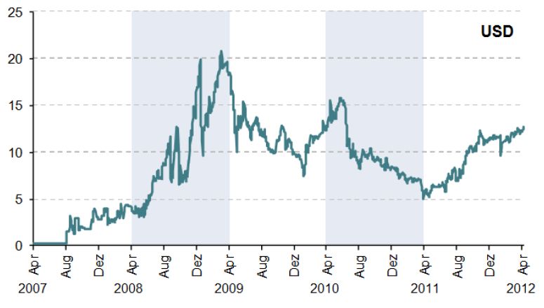
Contents

1 Description                                                                                 3

2 Introduction: Interest Rate Derivatives, Libor and Zero-Bond Curves                         4

3 Single-Curve Approach: One Curve Is Not Enough                                     7
  3.1 Single-Curve Bootstrapping . . . . . . . . . . . . . . . . . . . . . . . . . . 7
  3.2 The Single-Curve Approach in Light of the Financial Crisis . . . . . . . . . 11

4 Multi-Curve Approach: One Discount Curve and Distinct Forward Curves                       16
  4.1 Background . . . . . . . . . . . . . . . . . . . . . . . . . . . . . . . . . .         16
      4.1.1 Historical Background: New Regulations and the Rise of OIS . . . .               16
      4.1.2 Theoretical Background . . . . . . . . . . . . . . . . . . . . . . . .           17
  4.2 Basic Concept and Important Examples . . . . . . . . . . . . . . . . . . .             18
  4.3 Curve Construction . . . . . . . . . . . . . . . . . . . . . . . . . . . . . .         20
      4.3.1 OIS Curve Bootstrapping . . . . . . . . . . . . . . . . . . . . . . .            20
      4.3.2 Forward Curves Bootstrapping . . . . . . . . . . . . . . . . . . . .             22
  4.4 Validation of the Constructed Curves . . . . . . . . . . . . . . . . . . . .           24

5 Generalisation: Collateral in a Foreign Currency                                           26

6 Overview: Extensions of Interest Rate Models to the Multi-Curve World                      27

7 A Note on Libor: Its Rise, Scandal, Fall and Replacement                                   29

A Appendix                                                                             31
  A.1 Conventions . . . . . . . . . . . . . . . . . . . . . . . . . . . . . . . . . . 31
  A.2 Notation . . . . . . . . . . . . . . . . . . . . . . . . . . . . . . . . . . . . 31

   References                                                                                32

   Index                                                                                     34

Fraunhofer ITWM                      Progressing from Single- to Multi-Curve Bootstrapping        2|34
1 Description Description At the base of each financial market lies the valuation of its instruments. Until the financial crisis of 2007–2008, the single-curve approach and its bootstrapping technique were used to value linear interest rate derivatives. Due to lessons learnt during the crisis, the valuation process for derivatives has been fundamentally changed. The aim of this white paper is to explain the foundation of the single-curve approach, why and how the methodology has been changed to the multi-curve approach and how to handle the computations if the collateral is being held in another currency. Moreover, we provide a brief overview of how interest rate models, which are used to price non-linear interest rate derivatives, have been extended after the crisis. Finally, we take a look at the history and future of Libor, which will be phased out by the end of 2021. In particular, this document is an excellent starting point for someone who has had little or no prior exposure to this very relevant topic. At the time of publication, we were not aware of any similarly comprehensive resource. We intend to fill this gap by explaining in detail the fundamental concepts and by providing valuable background information. The last chapter about Libor can be studied independently from the remaining parts of this document. Fraunhofer ITWM Progressing from Single- to Multi-Curve Bootstrapping 3|34
2 Introduction: Interest Rate Derivatives, Libor and Zero-Bond                                                 Introduction:   Interest Rate
  Curves                                                                                                       Derivatives, Libor and Zero-
                                                                                                               Bond Curves

»Financial market« is a generic term for markets where financial instruments and com-
modities are traded. Financial instruments are monetary contracts between two or
more parties. A derivative is a financial instrument that derives its value from the perfor-
mance of one or more underlying entities. For instance, this set of entities can consist of
assets (such as stocks, bonds or commodities), indexes or interest rates and is itself called
»underlying«. Derivatives are either traded on an exchange, a centralised market where
transactions are standardised and regulated, or on an over-the-counter (OTC) market,
a decentralised market where transactions are not standardised and less regulated. OTC
markets are sometimes also called »off-exchange markets«. The OTC derivatives market
grew exponentially from 1980 through 2000 and is now the largest market for deriva-
tives. The gross market value of outstanding OTC derivatives contracts was USD 15 trillon
in 2016, which corresponds to one fifth of that year’s gross world product, see [3] and
[36]. As we will learn later in Section 4.1.1, additional regulations were imposed upon
the OTC market due to its role during the financial crisis of 2007–2008.

We are especially interested in valuing derivatives whose underlying is an interest rate
or a set of different interest rates and call these derivatives interest rate derivatives
(IRDs). One of the most important forms of risk that financial market participants face is
interest rate risk. This risk can be reduced and even eliminated entirely with the help of
IRDs. Furthermore, IRDs are also used to speculate on the movement of interest rates and
are mainly traded OTC. Around 67% of the global OTC derivatives market value arises
from OTC traded IRDs, see [3]. IRDs can be divided into two subclasses:

n   Linear IRDs are those whose payoff is linearly related to their underlying interest rate.
    Examples of this class are forward rate agreements, futures and interest rate swaps.1

    Until the financial crisis, the single-curve approach was used to price these IRDs. In
    Chapter 3, we will describe how it works, what the distinctive assumptions are and
    why they are flawed. Afterwards, in Chapter 4, we will discuss the multi-curve ap-
    proach, which is now market standard for pricing linear IRDs. We will then have a
    brief look at the multi-currency case in Chapter 5.

n   Non-linear IRDs are all the remaining instruments, i.e. those whose payoff evolves
    non-linearly with the value of the underlying. Basic examples are caps, floors and
    swaptions. However, this family of IRDs is very large and also includes very complex
    derivatives, such as autocaps, Bermudan swaptions, constant maturity swaps and zero
    coupon swaptions.

    We need interest rate models to price such IRDs, but they are not the focus of this
    paper. Nevertheless, in Chapter 6 we will provide a brief summary of how existing
    families of models were extended to the new framework due to the deeper market
    understanding and name the most relevant publications. Additionally, we point out
    links to results that were developed earlier in this paper.

 Aim: We want to construct interest rate curves that enable us to price any linear
 IRD of interest. For this purpose, we will use prices quoted on the market as input
 factors to a technique called »bootstrapping«.

Remark. The London Interbank Offered Rate (Libor) is the trimmed average of inter-
est rates estimated by each of the leading banks in London that they would be charged

 1 Forward  rate agreements and interest rate swaps will play a crucial role in this white paper and will be
    introduced in more detail later on.

Fraunhofer ITWM                              Progressing from Single- to Multi-Curve Bootstrapping                                     4|34
if they had to borrow unsecured funds in reasonable market size from one another. Cur- Introduction: Interest Rate
rently, it is calculated daily for five currencies (CHF, EUR, GBP, JPY, USD), each having Derivatives, Libor and Zero-
seven different tenors (1d, 1w, 1m, 2m, 3m, 6m, 12m). Hence, there exist in total 35 Bond Curves
distinct Libor rates. We omit the specification of the currency when not needed and write
∆-Libor for the Libor with tenor ∆. The banks contributing to Libor belong to the upper
part of the banks in terms of credit standing and were considered virtually risk-free prior
to the crisis. See Chapter 7 for more background information and for an explanation of
why Libor will be phased out by the end of 2021.
Remark. Similar reference rates set by the private sector are, for example, the Euro Inter-
bank Offered Rate (Euribor), the Singapore Interbank Offered Rate (Sibor) and the Tokyo
Interbank Offered Rate (Tibor). Everything we do is applicable to all interbank offered
rates. We refer solely to Libor due to the better readability and since this is an established
standard in the literature.
In the following, we assume that the considered IRDs only have one underlying interest
rate and that this rate is always Libor. Before we go into further details, we introduce
some basic definitions:
Definition 1. We consider a stochastic short rate model and denote the short rate
by r(s) at time point s. This rate is the continuously compounded and annualised interest
rate at which a market participant can borrow money for an infinitesimally short period
of time at s. The (stochastic) discount factor D(t, T ) between two time instants t and
T is the amount of money at time t that is »equivalent« to one unit of money payable at
time T and is given by !
Z T
D(t, T ) := exp − r(s)ds .
t
Just like exchange rates can be used to convert cash being held in different currencies
into one single currency, discount factors can be interpreted as special exchange rates
which convert cash flows that are received across time into another »single currency«,
namely into the present value of these future cash flows. Let us assume we know today
(t = 0) that we will receive X units of money in one year (T = 1). The present value
of this future cash flow can then be calculated as D(0, 1) · X. For obtaining the present
value in the case that we have several future cash flows, we just take the sum of the
respective present values.
Definition 2. A zero-coupon bond with maturity T (T -bond) is a riskless contract that
guarantees its holder the payment of one unit of money at time T with no intermediate
payments. The contract value at time t ≤ T is denoted by P (t, T ). Zero-coupon bonds
are sometimes also called »discount bonds«.
Note that P (T, T ) = 1 and if interest rates are positive we have for t ≤ T ≤ T 0
P (t, T ) ≥ P (t, T 0 ) .
For the valuation of linear IRDs we will need the prices of different zero-coupon bonds,
since it can be shown that
P (t, T ) = Et [D(t, T )] , (1)
where the expectation is taken with respect to the risk neutral pricing measure and the
filtration Ft , which encodes the market information available up to time t, see also
Section 4.1.2. Due to this crucial relation of discount factors and zero-coupon bonds, we
sometimes use expressions such as »we discount with P (t, T )«. In conclusion, we are
interested in the following curve:
Definition 3. The zero-bond curve at time t, with t ≤ T , is given by the mapping
T 7→ P (t, T ) .
This curve is sometimes also called »discount curve« or »term structure curve«.
Fraunhofer ITWM Progressing from Single- to Multi-Curve Bootstrapping 5|34Using the bootstrapping technique, which will be described in the next chapter, we Introduction: Interest Rate
first obtain a finite number of the zero-bond curve’s values from some given input data. Derivatives, Libor and Zero-
Roughly speaking, in a bootstrap calculation we determine a curve C : T 7→ C(T ) iter- Bond Curves
atively, where we get the unknown point C(Ti ) at Ti by a calculation that depends on
previous points of the curve, {C(Tj ) : j < i}. Afterwards, we use this finite number of
values to generate the rest of the curve via inter- and/or extrapolation techniques. So,
essentially, »bootstrapping« refers to forward substitution in the context of zero-bond
curve construction.
Remark. We want to stress that when we use the term »bootstrapping«, we do not refer
to the statistical method, let alone to any of its many other meanings. Usually, bootstrap-
ping refers to a self-starting process that is supposed to proceed without external input.
It is, by the way, also the origin of the term »booting«, used for the process of starting
a computer by loading the basic software into the memory which will then take care of
loading other software as needed. Etymologically, the term appears to have originated in
the early 19th-century United States, particularly in the phrase »pull oneself over a fence
by one’s bootstraps«, to mean an absurdly impossible action.
Fraunhofer ITWM Progressing from Single- to Multi-Curve Bootstrapping 6|343 Single-Curve Approach: One Curve Is Not Enough Single-Curve Approach: One
Curve Is Not Enough
Assumption: All linear IRDs depend on only one zero-bond curve.
Procedure: With this single zero-bond curve we
1. calculate the forward rates with which we obtain the future cash flows and
2. discount these future cash flows
at the same time to price our linear IRD of interest.
For the construction of this curve it is allowed to use any set of liquid linear IRDs on
the market with increasing maturities and which have Libor as an underlying. Liquid
instruments are those with negligible bid-ask spread, which basically means that supply
meets demand, so that they can be converted into cash quickly and easily for full market
price. In particular, the allowed sets of instruments do not have to be homogeneous,
i.e. they can have different Libor indexes as underlying, such as 1m-Libor, 3m-Libor . . .
It is important to realise that:
n Until the financial crisis of 2007–2008, Libor was seen as a good proxy for the theo-
retical concept of the risk-free rate, which motivated its usage for discounting.
n The usage of the same curve to discount the cash flows is a modelling choice and not
a contractual obligation and thus is theoretically open to debate.
As we will see, these two points are crucial differences to the multi-curve approach,
which is the method recommended by leading experts in the field, see for instance [15],
where Henrad first proposed a different approach in 2007, and also [6], [25] and [27].
Nevertheless, we first start with the single-curve approach as it not only deepens our
general understanding by outlining the historic evolution, but also uses a bootstrapping
technique that will be relevant for the multi-curve approach later on.
3.1 Single-Curve Bootstrapping
In the following, τ (t, T ) denotes the time period in years between time point t and T
according to a specific day count convention. We assume the Actual/360 one, as Libor for
all currencies except GBP (there it is the Actual/365 one) is based on it and, in general, it
is the most prevalent day count convention for money market instruments with maturity
1
below one year. It is determined by the factor 360 ·Days(t, T ), i.e. one year is assumed to
consist of 360 days, see [29].
Before we illustrate the bootstrapping procedure, we would like to introduce the concept
of a simply compounded spot rate L(t, T ). By an arbitrage argument2 , one unit of
currency at time T should be worth P (t, T ) units of currency at time t, see (1). Hence,
we want that the following equation holds:
1 = P (t, T ) 1 + τ (t, T ) · L(t, T ) , (2)
2 An arbitrage opportunity is the possibility to make a riskless profit in a financial market without net invest-
ment of capital. The no-arbitrage principle states that a mathematical model of a financial market should
not allow any arbitrage possibilities.
Fraunhofer ITWM Progressing from Single- to Multi-Curve Bootstrapping 7|34i.e. we assume that L(t, T ) is a riskless lending rate. This leads us to the following Single-Curve Approach: One
definition: Curve Is Not Enough
Definition 4. The simply compounded spot rate at time t for maturity T is defined
as
1 − P (t, T )
L(t, T ) := . (3)
τ (t, T ) · P (t, T )
Important simply compounded spot rates are the market Libor rates, which motivates the
above notation L(t, T ).
Definition 5. In a fixed for floating interest rate swap two parties periodically ex-
change interest rate payments on a given notional amount N . One party pays a fixed
rate whereas the other pays a floating rate. These instruments are particularly useful
for reducing or eliminating the exposure to interest rate risk. According to the market
conventions of a given currency the fixed payment schedule has standard periods, for
instance one year for EUR or six months for USD, see [29]. We call the sum of fixed
payments the fixed leg and the sum of the floating payments the floating leg.
Remark. In a general interest rate swap (IRS), each of the two parties has to pay either
a fixed or a floating interest rate on a given notional amount N to its counterparty. An
IRS is traded OTC and its notional amounts are never exchanged, as the term »notional«
suggests.3 The most common form of an IRS is a fixed for floating swap and the least
common form is a fixed for fixed swap. IRSs constitute with 60% the largest part of
the global OTC derivatives gross market value in 2017, see [3]. Consequently, they also
represent by far the largest part of all OTC traded IRDs.
Prior to the financial crisis of 2007–2008, we were, for example, provided with the rates
of Fig. 1 for bootstrapping the discount factors. So, in this case, Libor rates L(0, T ), T ∈
{1m, 3m, 6m, 12m} are used as input rates until 12 months and swap fixed rates S(0, T ),
T ∈ {2y, 3y, . . . , 30y, 40y, 50y}, from 2 years to 50 years. As mentioned previously, any
set of liquid vanilla interest rate instruments on the market with increasing maturities
could be used, e.g. in addition to the ones above also mid-term futures or forward rate
agreements on 3m-Libor.
Index Type Duration
1 Libor rate 1 month
2 Libor rate 3 months
3 Libor rate 6 months
4 Libor rate 12 months
5 Swap fixed rate 2 years
6 Swap fixed rate 3 years
.. .. ..
. . .
32 Swap fixed rate 29 years
33 Swap fixed rate 30 years
34 Swap fixed rate 40 years
Fig. 1: Input rates for bootstrap-
35 Swap fixed rate 50 years ping prior to the financial crisis
Clearly, the resulting bootstrapped curve is a curve, where the prices of the instruments
used as an input to the curve coincide with the prices that are calculated using this curve
when valuing these same instruments.
3 Hence, it does not make too much sense to estimate the IRS market size and risk by adding up the notional
values of all outstanding IRSs. Unfortunately, this is still a common practice and even used in regulatory
calculations, see also [14].
Fraunhofer ITWM Progressing from Single- to Multi-Curve Bootstrapping 8|34Using the bootstrapping technique, we are now going to extract N = 35 distinct grid Single-Curve Approach: One
points of the zero-bond curve P (0, ·) from the above N distinct rates. These grid points Curve Is Not Enough
will be the values P (0, T ) with
T ∈ {1m, 3m, 6m, 12m, 2y, 3y, . . . , 30y, 40y, 50y} .
To this end, different calculations apply – one for T ≤ 1y, one for 1y < T ≤ 30y and one
for 30y < T :
n For T ≤ 1y:
From equation (2) follows immediately that
1
P (0, T ) = .
1 + τ (0, T )L(0, T )
Note that in the case of EUR and GBP Libor, the fixing date of Libor corresponds to
its value date, i.e. the rate is set on the same day that the banks contribute their
submissions. However, for all currencies other than EUR and GBP the value date will
fall two London business days after the fixing date, see [29]. If this subsequent date is
(a) not a market holiday, we have to consider the overnight rate rON for the first
day and the spot next rate rSN for the day after to get the exact bond prices, see
[20]. So in this case we would get
1
P (0, T ) = .
1 + τ (0, 1d)rON + τ (1d, 2d)rSN + τ (2d, T )L(0, T )
(b) a market holiday, the value date will roll onto the next date which is a normal
business day both in London and in the principal financial centre of the relevant
currency.
n For 1y < T ≤ 30y:
From one year onwards, we use swap fixed rates to calculate the bond prices. We
consider swap rates that are quoted annually and where the fixed rate is paid annu-
ally, too, as is the case in the EUR market, see [29]. The starting point is again an
equation: For instance, when T = 2y we start with
1 = S(0, 2y)τ (0, 1y)P (0, 1y) + τ (1y, 2y)S(0, 2y) + 1 P (0, 2y) .
This treats the swap as a 2-year S(0, 2) fixed-rate bullet bond priced at par value of 1.
A bullet bond is a debt instrument whose entire principal value is paid all at once on
the maturity date, as opposed to amortizing the bond over its lifetime. It cannot be
redeemed prior to maturity.
All payments on this hypothetical bond prior to the maturity date – which is in this
case only one payment after one year – are multiplied by the corresponding bond
price. At maturity we discount the last payment and the repaid principal with the
unknown factor P (0, 2y). Hence, we obtain
1 − S(0, 2y)τ (0, 1y)P (0, 1y)
P (0, 2y) = .
1 + τ (1y, 2y)S(0, 2y)
To get P (0, 3y), we start from
1 = S(0, 3y)τ (0, 1y)P (0, 1y) + S(0, 3y)τ (1y, 2y)P (0, 2y)
+ τ (2y, 3y)S(0, 3y) + 1 P (0, 3y) ,
Fraunhofer ITWM Progressing from Single- to Multi-Curve Bootstrapping 9|34and so on . . . So, in general we have Single-Curve Approach: One
Pn−1 Curve Is Not Enough
1 − S(0, T ) · i=1 τ (Ti−1 , Ti ) · P (0, Ti )
P (0, T ) = P (0, Tn ) = , (4)
1 + S(0, T ) · τ (Tn−1 , Tn )
where we write Tn to denote that the corresponding swap has a duration of n years
and we put T0 := 0. It is possible to solve the above equations for the different T at
once using matrix computations, as illustrated in [9].
Once again, we have to pay attention to different market conventions: For example,
in the USD market the fixed rate is payed semi-annually. However, we do not have,
for instance, a 1y6m swap fixed rate to calculate P (0, 1y6m). The simple solution
is to interpolate the missing swap fixed rates with a suitable interpolation technique,
see the next remark, and to apply a similar procedure as described for the next case,
30y < T , in more detail. The used interpolated rates are also referred to as »synthetic
rates« in the literature.
n For 30y < T :
The data for long durations is usually sparse. Therefore we use an iterative approach
for calculating the bond prices, where we obtain a value Pi (0, T ) in each iteration. Let
T = 40 and for i = 1 we set
1 40
P1 (0, 40) := .
1 + S(0, 40)
We proceed as follows:
1. Derive the bond prices for the years 31, . . . , 39 using log-linear interpolation, or any
other suitable interpolation technique, see the next remark, between P (0, 30) and
Pi (0, 40). We assume for now that the obtained values are the true ones.
2. Calculate Pi+1 (0, 40) as in equation (4) with the obtained values of the previous
step.
This routine is repeated until for the k-th repetition the obtained improvement is neg-
ligibly small, e.g.
|Pk+1 (0, 40) − Pk (0, 40)| < 10−8 .
For the following years, the same routine is applied.
After obtaining the bond prices at the given time points we can interpolate between
them to get the entire zero-bond curve.4
Remark. Usually, the interpolation is done on the logarithm of the bond prices using
one or the other interpolation method. In [30], the usage of different interpolation
methods for curve construction is discussed in detail. The authors provide some warning
flags and stress that natural cubic splines possess the non-locality property, since it uses
information from three time points. Non-locality means that if the input value at time
point ti is changed, the interval (ti−l , ti+u ), where the values of the curve change, is
rather large. The method choice is always subjective and needs to be decided on a case
by case basis.
As explained previously, in the single-curve approach we only use the information of this
unique zero-bond curve to price any linear IRD in a given currency.
4 SeeSection 4.3.2 for an alternative, the so-called »best fit approach«, which is being used by most central
banks.
Fraunhofer ITWM Progressing from Single- to Multi-Curve Bootstrapping 10|343.2 The Single-Curve Approach in Light of the Financial Crisis Single-Curve Approach: One
Curve Is Not Enough
In the following, we illustrate in the first proof of Lemma 3.1 how the usage of this one
curve works and provide a brief explanation why this procedure is not recommendable.
This motivates the usage of the multi-curve approach, which will be covered in Chapter 4.
Definition 6.
n A standard forward rate agreement (FRA) is a contract involving three time in-
stants: (i) the current time t, (ii) the expiry time Ti−1 and (iii) the maturity time Ti , with
t ≤ Ti−1 < Ti .
n The contract gives its holder an interest rate payment for the period between Ti−1
and Ti at maturity Ti , which corresponds to the difference between the fixed rate
L(t, Ti−1 , Ti ) and the floating spot rate L(Ti−1 , Ti ).
n L(t, Ti−1 , Ti ) is the risk-free rate for the time interval [Ti−1 , Ti ] determined at time t
and we call it the simply compounded forward rate or the FRA rate.
Lemma 3.1
Using the single-curve approach we get
1 P (t, Ti−1 )
L(t, Ti−1 , Ti ) = −1 . (5)
τ (Ti−1 , Ti ) P (t, Ti )
To show this we provide two proofs. The first one illustrates how we get the above
expression and the second one uses a replication argument to which we will come back
later.
Proof 1. Here we follow the proof of [7]. Let N denote the contract nominal value and
K the simply compounded forward rate with expiry time Ti−1 and maturity time Ti , i.e.
K = L(t, Ti−1 , Ti ). At time Ti one receives τ (Ti−1 , Ti )KN units of currency and pays
τ (Ti−1 , Ti )L(Ti−1 , Ti )N . The payoff of the contract at time Ti is therefore
FRA(t, Ti−1 , Ti , N ) = N τ (Ti−1 , Ti ) K − L(Ti−1 , Ti )
(3)
1
(6)
= N τ (Ti−1 , Ti )K − +1 .
P (Ti−1 , Ti )
Because of the assumption that we are using the single-curve approach we can discount
the cash flows with the same curve. Note that the amount 1/P (Ti−1 , Ti ) at time Ti is
worth one unit of money at time Ti−1 . One unit of money at time Ti−1 is in turn equal
to an amount of P (t, Ti−1 ) at time t. On the other hand, the amount τ (Ti−1 , Ti )K + 1
from (6) at time Ti is worth P (t, Ti )τ (Ti−1 , Ti )K + P (t, Ti ) at time t. The total value of
the forward rate agreement at time t is
N P (t, Ti )τ (Ti−1 , Ti )K − P (t, Ti−1 ) + P (t, Ti ) .
If we equate this to zero for no-arbitrage reasons and solve for K we obtain the above
statement.
Proof 2. At first, we construct two separate strategies at different time points:
Fraunhofer ITWM Progressing from Single- to Multi-Curve Bootstrapping 11|34Time FRA-Strategy Bond-Strategy Single-Curve Approach: One
t • buy one FRA • sell one Ti−1 -bond Curve Is Not Enough
• buy PP(t,T i−1 )
(t,Ti ) Ti -bonds
cash flow 0 cash flow 0
Ti−1 • invest 1 at L(Ti−1 , Ti ) • pay back Ti−1 -bond
cash flow −1 cash flow −1
Ti • receive from investment: • receive from Ti -bonds:
P (t,Ti−1 )
1 + L(Ti−1 , Ti ) · τ (Ti−1 , Ti ) P (t,Ti )
• receive from FRA:
(L(t, Ti−1 , Ti ) − L(Ti−1 , Ti )) · τ (Ti−1 , Ti )
P (t,Ti−1 )
cash flow 1 + L(t, Ti−1 , Ti ) · τ (Ti−1 , Ti ) cash flow P (t,Ti )
Due to the no-arbitrage assumption we get
P (t, Ti−1 )
1 + L(t, Ti−1 , Ti ) · τ (Ti−1 , Ti ) =
P (t, Ti )
1 P (t, Ti−1 )
⇔ L(t, Ti−1 , Ti ) = −1 .
τ (Ti−1 , Ti ) P (t, Ti )
Remark. Using (3) and Lemma 3.1 it follows that the simply compounded spot rate is
equal to the simply compounded forward rate if t = Ti−1 , i.e.
1 − P (t, Ti )
L(t, Ti ) = = L(t, t, Ti ) . (7)
τ (t, Ti ) · P (t, Ti )
In the literature, the simply compounded spot rate L(t, Ti ) is sometimes defined as the
value of the simply compounded forward rate L(t, Ti−1 , Ti ) with t = Ti−1 . However,
we started with the simply compounded spot rate and derived the value of the simply
compounded forward rate in Lemma 3.1 because the proofs provide us with a deeper
understanding of the single-curve approach, as we will realise very soon.
At this point, we already introduce the concept of the net present value, which will be
covered in more detail in Section 4.1.2:
Definition 7. We define the net present value (NPV) at time t of a financial transaction
with net cash flows5 Cash(Ti ) at time points Ti , i ∈ {1, . . . , M }, by
M
X
NPV(t) := P (t, Ti )Eit [Cash(Ti )] , (8)
i=1
where Eit [·] denotes the expectation under the Ti -forward measure associated with the
risk-free zero-coupon bond P (t, ·) and the filtration Ft .
Example 1. The NPV of a Libor swap’s floating leg at time t is given by
M
X
NPV(t) = P (t, Ti )L(t, Ti−1 , Ti )τ (Ti−1 , Ti ) ,
i=1
5 »Netcash flow« refers to the difference between cash inflows and cash outflows in a given period of time.
Accordingly, the »net present value« is the difference between the present value of cash inflows and the
present value of cash outflows in a given period of time.
Fraunhofer ITWM Progressing from Single- to Multi-Curve Bootstrapping 12|34where TM denotes the maturity date of the swap. Hence, it is given by simply summing Single-Curve Approach: One
up the values of the single floating payments discounted with the corresponding zero- Curve Is Not Enough
coupon bond price, compare the paragraph after Definition 1.
Lemma 3.2
For the NPV of a Libor swap’s floating leg at time t it holds
NPV(t) = 1 − P (t, TM ) . (9)
Proof.
M
X
NPV(t) = P (t, Ti )L(t, Ti−1 , Ti )τ (Ti−1 , Ti )
i=1
M
(5) X P (t, Ti−1 )
= P (t, Ti ) −1
i=1
P (t, Ti )
M
X
= P (t, Ti−1 ) − P (t, Ti )
i=1
= 1 − P (t, TM )
In particular, (9) shows that NPV(t) does not depend on the tenor structure of the swap.
Definition 8. A tenor basis swap is a floating for floating IRS. Typically floating cash
flows from two different Libor indices of the same currency are exchanged, e.g. 3m-Libor
vs. 6m-Libor cash flows, which we denote by 3m-6m-Libor tenor basis swap. A so-called
»tenor basis spread« s is added to the Libor index with the lower index to quote a tenor
basis spread with a fixed maturity at par.
Definition 9. An overnight (index) rate is usually computed as a weighted average of
overnight unsecured lending between large banks. Important examples are the effective
Federal Funds Rate (FFR) for USD, the Euro OverNight Index Average (EONIA) and the
Sterling OverNight Index Average (SONIA). In some countries, central banks publish a
target overnight rate to influence monetary policy, for instance in the US. In contrast to
Libor, it is based on actual transactions by definition.
Definition 10. An overnight indexed swap (OIS) is an interest rate swap where the
floating payment is calculated via an overnight rate. The fixed rate of the OIS is typically
an interest rate considered less risky than the corresponding Libor rate because it contains
lower counterparty risk. Please note that the term »OIS rate« refers to the fixed rate of
the OIS and not to the reference rate.
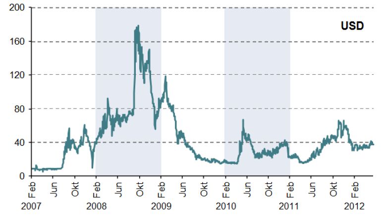
Remark. The Libor-OIS spread is seen as a measure for the health of banks since it
reflects what banks believe is the risk of default when lending to another bank. Prior to
2007, the spread between the two rates used to be as little as 0.01%. A widening of the
gap, as it was the case during the crisis, is a sign that the financial sector is stressed. In
early 2018, at the time of writing this document, it was close to 0.6% – its highest level
during the past ten years. However, the current spread is only observable in the US and
analysts claim that its increase is not critical and exists only due to effects of recent fiscal
policies.
Equations (5) and (9) imply that in the single-curve approach both Libor-OIS spreads and
tenor basis spreads are always equal to zero, which can be verified empirically. However,
Fraunhofer ITWM Progressing from Single- to Multi-Curve Bootstrapping 13|34Single-Curve Approach: One
Curve Is Not Enough
Fig. 2: 3m-Libor-OIS spread (1y);
source: Bloomberg
Fig. 3: 3m-Libor vs. 6m-Libor
tenor basis spread (5y); source:
Bloomberg
the financial crisis of 2007–2008 has shown that this is not the case, as Fig. 2 and 3
indicate. For further visualisations see also [26].
We make two decisive observations that motivate the usage of the multi-curve approach,
which will be introduced in the next chapter:
n In the second proof of Lemma 3.1 the FRA has tenor ∆F RA = Ti − Ti−1 , whereas the
bonds that are bought at time point t have tenor ∆Bonds = Ti − t and therefore for
t 6= Ti−1 we have
∆F RA 6= ∆Bonds . (10)
n On the other hand we know since the crisis that financial instruments with a longer
tenor have larger liquidity and counterparty credit risks. These risks are defined from
the viewpoint of a specific market participant A as follows:
n Market liquidity risk is the risk that A will have difficulty selling an asset without
incurring a loss. It is typically indicated by an abnormally wide bid-ask spread. It can
be caused by A itself, if its position is large relative to the market, or exogenously
by a reduction of buyers in the marketplace. In the subprime mortgage crisis, which
initiated the financial crisis of 2007–2008, rapid endorsement and later abandon-
ment of complicated structured financial instruments such as collateralised debt
obligations (CDOs) lead to an immense drop in market prices and thereby to a loss
of liquidity. Market liquidity risk is positively correlated to funding liquidity risk.
n Funding liquidity risk is the risk that A will become unable to settle its obligations
with immediacy over a specific time horizon and, as a result, will have to liquidate
a position at a loss that it would keep otherwise. In the run up to the financial
crisis, many banks were engaging in funding strategies that heavily relied on short-
term funding thus significantly increasing their exposure to funding liquidity risk,
see [21]. When banks such as Bear Stearns and Lehman Brothers started to look
Fraunhofer ITWM Progressing from Single- to Multi-Curve Bootstrapping 14|34vulnerable, their clients risked losing capital during a bankruptcy and they started Single-Curve Approach: One
to withdraw money and unwind positions, which lead to a bank run. This in turn Curve Is Not Enough
increased market illiquidity with bid-ask spreads widening and as a consequence
prices dropped.
n Counterparty (credit) risk or default risk, is the risk that a financial loss will be
incurred if one of A’s counterparties does not fulfil its contractual obligations in a
timely manner. For instance, when Lehman Brothers filed for bankruptcy it was a
counterparty to 930,000 derivative transactions which represented approximately
5% of global derivative transactions according to [18].
Since financial instruments with a longer tenor have larger liquidity and counterparty
credit risks, it makes no sense that the NPV of a Libor swap’s floating leg at time t does
not depend on the tenor of the swap. However, this is being implied by Lemma 3.2.
One way to deal with the risk inconsistency mentioned in the second observation is
to model these risks explicitly, so that the different rates become compatible with one
another. Another way to tackle the problem is to segment market rates according to
their tenor.
The second approach is suggested by Morini in [27], where he argues that an IRD with
tenor ∆ should only be replicated with IRDs of the same tenor ∆. Therefore, he implicitly
does not recommend the procedure in the second proof of Lemma 3.1, as there we have
in general ∆F RA 6= ∆Bonds , see (10).
Conclusion: The need to consider liquidity and counterparty credit risks when pric-
ing IRDs is one of the key insights of the financial crisis of 2007–2008. This insight
constitutes the decisive turning point of the pricing approach for IRDs.
Fraunhofer ITWM Progressing from Single- to Multi-Curve Bootstrapping 15|344 Multi-Curve Approach: One Discount Curve and Distinct Multi-Curve Approach: One
Forward Curves Discount Curve and Distinct
Forward Curves
The underlying idea of the multi-curve approach is to segment market rates according
to their tenor. Thereby, we overcome the risk inconsistency discussed at the end of the
last section. Before we illustrate this concept with some examples in Section 4.2, we first
provide some historical and theoretical background to motivate and specify important
details.
4.1 Background
4.1.1 Historical Background: New Regulations and the Rise of OIS
After the crisis, many regulatory steps were taken in order to address the solvency and
liquidity problems that arose during the crisis. Important regulations are the Dodd-Frank
Act and Basel III, which include provisions that tighten bank capital requirements, intro-
duce leverage ratios and establish liquidity requirements.
Similarly, there has also been a higher attention on the counterparty credit risk. The
following two key instruments attempt to reduce this risk:
n Collateral agreements: A collateral agreement is an additional contract to a main
contract where the terms for the exchange of the collateral as a security are specified.
There is a wide range of eligible collaterals which goes from cash to government or
corporate bonds and more rarely bullions. If the NPV of the main contract is positive
for A and exceeds a certain threshold by X, party A receives the collateral with value
X from party B. As long as B is not in default it remains the owner of the collateral
from an economic point of view and A needs to pass on coupon payments, dividends
and any other cash flows to B. If the difference between the NPV and the value of the
collateral position is in excess of the Minimum Transfer Amount (MTA), extra collateral
needs to be posted. Collateralised transactions pose less counterparty risk because
the collateral can be used to recoup any losses.
n Central (clearing) counterparty (CCP): In the aftermath of the crisis, authorities
tried to push derivatives markets towards collateralisation of OTC transactions. The
Dodd-Frank Act and the European Market Infrastructure Regulation (EMIR) intend to
mitigate counterparty credit risk through the creation of CCPs. A CCP is a financial
institution that interposes itself between counterparties of contracts, becoming the
buyer to every seller and the seller to every buyer. It provides greater transparency of
the risks, reduced processing costs and established processes in case of a member’s
default, see [34]. The most important aspect of central clearing is the multilateral
netting of transactions between market participants, which simplifies outstanding
exposures compared to a complex web of bilateral trades.
We illustrate this effect with the simplest possible example: We have three market
participants, A, B and C. A has to post a collateral of Y to B, B has to post a
collateral of Y to C and C has to post a collateral of Y to A. If we consider the exact
same situation only with a central counterparty in place, which is allowed to apply
multilateral netting, then no party has to post a collateral any more. This is the case,
since each of the three parties posts and receives the same amount of collateral.
However, one should not forget that CCPs cannot fully eliminate counterparty credit
risk. Furthermore, they concentrate risk, their probability of default is positive and they
can be sources of financial shocks if they are not properly managed.
Fraunhofer ITWM Progressing from Single- to Multi-Curve Bootstrapping 16|34For transactions that are not centrally cleared by a CCP, regulators also impose the inclu- Multi-Curve Approach: One
sion of a Credit Support Annex (CSA), a document where the collateralisation terms Discount Curve and Distinct
and conditions are determined in detail. According to the International Swaps and Forward Curves
Derivatives Association (ISDA), cash represents around 77% of collateral received and
around 78% of collateral delivered against non-cleared derivatives in 2014, see [17]. The
collateral rate which is being paid on cash collateral is also the effective funding rate
for the derivative, as shown in [8]. This means that the appropriate rate to discount cash
flows when valuing a collateralised trade corresponds to the collateral rate, which is in
most cases an overnight rate. For instance, in the ISDA CSA for OTC derivative transac-
tions, the collateral rate is usually determined as the OIS rate, i.e. the fixed rate of the
OIS. Hence, we assume in the sequel that the collateral rate is the OIS rate.
OIS is the most prevalent choice amongst collateral rates because it is seen as the best
estimate of the theoretical concept of the risk-free rate. A good approximation of the
risk-free rate is desirable, since the collateral has effectively eliminated counterparty risk.
As mentioned before, until the financial crisis Libor was also assumed to be a good such
estimate, but during the crisis the Libor-OIS spread spiked to an all-time high of 3.64%.
That Libor cannot be assumed to be risk-free was also discussed in the media in the
aftermath of the Libor manipulation scandal of 2011, see [4] and Chapter 7. Whereas
the overnight rates on which OIS are based are averages of actual transactions, Libor
often just reflects the opinion of several banks at which rate other banks would let them
borrow money, see Chapter 7.
4.1.2 Theoretical Background
Definition 4.1
With the risk neutral pricing approach, see [23], we obtain the net present value
(NPV) at time t of a financial transaction with net cash flows Cash(Ti ) at time points Ti ,
i ∈ {1, . . . , M }, by "M #
X
NPV(t) := Et D(t, Ti ) · Cash(Ti ) ,
i=1
where
n as before, r(s) denotes the short rate at time s
n D(t, T ) denotes the discount factor
!
Z T
D(t, T ) := exp − r(s)ds
t
n and the expectation is taken with respect to the risk neutral pricing measure and
the filtration Ft , which encodes the market information available up to time t.
Unfortunately, we do not know D(t, T ) at t. As suggested earlier in (1), there is a useful
relation between D(t, T ) and the zero-coupon bond corresponding to r(s)
" !#
Z T
P (t, T ) = Et [D(t, T )] = Et exp − r(s)ds .
t
By a change of numeraire to P (t, ·) we obtain
M
X
NPV(t) = P (t, Ti )Eit [Cash(Ti )] , (11)
i=1
Fraunhofer ITWM Progressing from Single- to Multi-Curve Bootstrapping 17|34where Eit [·] denotes the expectation under the Ti -forward measure associated with the Multi-Curve Approach: One
risk-free zero-coupon bond P (t, ·) and the filtration Ft .6 Discount Curve and Distinct
Forward Curves
We can now use (11) to calculate the NPV if we know to which interest rate the short
rate r(s) corresponds. In [32], it is shown that if the transaction is
(a) uncollateralised with no counterparty credit risk then r(s) corresponds to the coun-
terparty’s funding rate.
(b) completely collateralised then r(s) corresponds to the collateral rate.
The first case is of rather theoretical nature, since in practice, uncollateralised transactions
usually involve counterparty credit risk. Note that if we are in the first case, then we
would again use Libor in the interbank sector, just as in the single-curve approach.
We will assume in the following that we are in the second case, i.e. that our contracts
are collateralised, as this is standard nowadays. For example, in 2014 around 97% of
non-cleared credit derivatives and 91% of non-cleared equity derivatives were already
using CSAs, see [17]. In this case it is reasonable to assume that the collateral rate is the
OIS rate as, again, this is market standard, see [12].
4.2 Basic Concept and Important Examples
In conclusion, in the multi-curve approach we first build one single zero-bond curve from
OIS rates. We continue to denote this zero-bond curve by P (t, ·) and will explain its
construction later in Section 4.3.1.
Apart from the zero-bond curve, we segment the interest rate market with respect to
the different tenor structures of its derivatives. We use in each partial market a separate
interest rate structure to value its IRDs. For instance, we use FRAs with 6m-tenor for the
first two years and afterwards Libor swaps with 6m-tenor to account for the forward
rates with 6m-tenor. This will be illustrated in Section 4.3.2.
Assumption: The IRD market should be segmented according to the tenor of its
products.
Procedure: For pricing a linear IRD with tenor ∆, we
1. calculate the future cash flows with the forward rate curve of tenor ∆ and
2. discount these future cash flows with a unique zero-bond curve.
Due to the importance of tenors in the multi-curve approach and for the sake of consis-
tency, we alter the notation of the simply compounded spot rate L(T − ∆, T ) of (3) to
L∆ (T − ∆, T ).
Definition 11. Consider a linear IRD with cash flows
Cash(Ti ) := αi + βi · L∆ (Ti−1 , Ti ) ,
where αi , βi ∈ R for i = 1, . . . , M and T1 < . . . < TM with Tj − Tj−1 = ∆ for
6 In fact, this is how we defined the NPV earlier in Definition 7.
Fraunhofer ITWM Progressing from Single- to Multi-Curve Bootstrapping 18|34j = 2, . . . , M . With (11) we obtain Multi-Curve Approach: One
M h i Discount Curve and Distinct
Forward Curves
X
NPV(t) = P (t, Ti ) · Eit Cash(Ti )
i=1
(12)
M
X h i
= P (t, Ti ) · αi + βi · Eit L∆ (Ti−1 , Ti ) .
i=1
h i
We set L∆ (t, Ti−1 , Ti ) := Eit L∆ (Ti−1 , Ti ) and call the curve given by the mapping
T 7→ L∆ (t, T − ∆, T ) the ∆-fixing curve at time t.
Remark. In the literature, one often defines the ∆-fixing curves using risky zero-bond
curves P ∆ (t, ·) by
∆
1 P (t, Ti−1 )
L∆ (t, Ti−1 , Ti ) := − 1 .
τ (Ti−1 , Ti ) P ∆ (t, Ti )
This is motivated by (5). We then have all curves of interest, i.e. the zero-bond curve and
the different forward curves, in »zero-bond form«. Here in this white paper, we omit this
practice as it would not add any extra insights.
For valuing an IRD as in the above definition we need to know the specific ∆-fixing curve.
Therefore, we would like to discuss the value of a FRA:
Example 2. For the standard FRA, which we have introduced in Definition 6, the pay-
ment date is assumed to be Ti , so at time Ti we have the payoff
F RAstd := F RAstd (t, Ti−1 , Ti , N ) := N τ (Ti−1 , Ti ) K − L∆ (Ti−1 , Ti ) ,
where K is the FRA rate, N the nominal value and ∆ = Ti − Ti−1 . With (11), the NPV at
time t is given by
h i
N P VF RAstd = P (t, Ti ) · Eit N τ (Ti−1 , Ti ) K − L∆ (Ti−1 , Ti )
h i
= P (t, Ti ) · N τ (Ti−1 , Ti ) K − Eit L∆ (Ti−1 , Ti ) .
Since K is chosen such that N P VF RAstd = 0 we get
h i
L∆ (t, Ti−1 , Ti ) := Eit L∆ (Ti−1 , Ti ) = K . (13)
Example 3. The actual FRA traded on the market, however, has payment date Ti−1 and
is discounted with the floating spot rate, i.e. at time Ti−1 we have the payoff
K − L∆ (Ti−1 , Ti )
F RAmkt := F RAmkt (t, Ti−1 , Ti , N ) := N τ (Ti−1 , Ti ) .
1 + τ (Ti−1 , Ti )L∆ (Ti−1 , Ti )
Note that the discounting with the floating spot rate is not a modelling choice but spec-
ified in the contract itself. Mercurio shows in [25] that the NPV at time t is given by
1 + K · τ (Ti−1 , Ti )
N P VF RAmkt = P (t, Ti−1 )N exp(C(t, Ti−1 )) − 1 ,
1 + L∆ (t, Ti−1 , Ti )τ (Ti−1 , Ti )
where exp(C(t, Ti−1 )) is called »convexity adjustment« and depends on the model. He
further proves that under reasonable model assumptions and if the difference between
forward Libor rates and corresponding OIS rates remains fairly constant, which is usually
the case, then the value of C(t, Ti−1 ) is negligibly small and we further have
N P VF RAmkt ≈ N P VF RAstd = P (t, Ti ) · N τ (Ti−1 , Ti ) K − L∆ (t, Ti−1 , Ti ) , (14)
which again results in L∆ (t, Ti−1 , Ti ) = K.
Fraunhofer ITWM Progressing from Single- to Multi-Curve Bootstrapping 19|34Remark. Note that FRA contracts are quoted on the market in terms of the FRA equilib- Multi-Curve Approach: One
rium rates. They are also included into rates of futures, interest rate swaps and tenor basis Discount Curve and Distinct
swaps. Therefore, the different FRA curves can be extracted from market quotations. Forward Curves
Example 4. To illustrate the use of Definition 11 we consider a 6m-Libor fixed for floating
swap over the term of two years. We will use the resulting pricing formula to construct
the 6m-fixing curve in Section 4.3.2. For simplicity, we drop the usage of day count
conventions at this point and assume that the payments take place semi-annually. We
recommend to compare the following procedure to the one used in the first proof of
Lemma 3.1, where we applied the single-curve approach to price a standard FRA.
n The fixed party pays at time i · 6m the cash flows
Cash(i · 6m) = S(0, 2y) · 6m = αi + βi · L6m ((i − 1) · 6m, i · 6m) ,
with the swap fixed rate S(0, 2y), αi = S(0, 2y) · 6m and βi = 0. With (12) we get
the fixed leg
X4
NPV(0) = S(0, 2y) · 6m P (0, i · 6m) .
i=1
n The variable party pays at time i · 6m the cash flows
Cash(i · 6m) = L6m ((i − 1) · 6m, i · 6m) · 6m = αi + βi · L6m (Ti−1 , Ti ) ,
with αi = 0 and βi = 6m. With (12) and the 6m-fixing curve we get the floating leg
4
X
NPV(0) = P (0, i · 6m) · 6m · L6m (0, (i − 1) · 6m, i · 6m) .
i=1
n So, in summary we get
P4
i=1 P (0, i · 6m) · L6m (0, (i − 1) · 6m, i · 6m)
S(0, 2y) = P4 .
i=1 P (0, i · 6m)
In general, i.e. with day count conventions and different fixed and floating payment
dates, we obtain
Pñ
P (0, T̃i )τ (T̃i−1 , T̃i )L∆ (0, T̃i−1 , T̃i )
S(0, Tn ) = i=1 Pn , (15)
i=1 τ (Ti−1 , Ti )P (0, Ti )
where T = {T1 , . . . , Tn } is the time structure of the fixed cash flows and T̃ ∆ = {T̃1∆ , . . . , T̃ñ∆ =
∆
Tn } is the time structure of the floating cash flows with T̃i+1 = T̃i∆ + ∆, i = 1, . . . , ñ − 1.
4.3 Curve Construction
We start with the construction of the zero-bond curve from OIS rates in Section 4.3.1, as
this curve will be used to construct the forward curves in Section 4.3.2.
4.3.1 OIS Curve Bootstrapping
In the sequel we follow [20] and [9]. The starting point of the multi-curve approach is
always the construction of a zero-bond curve P (t, ·). We denote by
Fraunhofer ITWM Progressing from Single- to Multi-Curve Bootstrapping 20|34Multi-Curve Approach: One
Discount Curve and Distinct
Forward Curves
Fig. 4: Daily effective Federal
Funds Rate; source: St. Louis Fed
n N the number of business days in a given period
n τi the year fraction between the business day i and the next business day, for example
we normally have for i being a Friday τi = 3/(number of days in the specific year)
n REFi the reference rate published for business day i which is valid until the next busi-
ness day and usually published on business day i + 1.
The paid interest over this period is
N
Y
(1 + τi · REFi ) − 1 .
i=1
Note that the final settlement of an OIS occurs one day after the maturity date of the OIS
due to the delay of publishing the reference rate for the maturity date, see [29].
A special feature of OIS rates is the quasi-static behaviour of reference rates between
Monetary Policy Meeting Dates. Another speciality is that there are often seasonality
effects observable at each quarter or end of the year, see Fig. 4.
We assume that the seasonality adjustment is built into the rates REFi by adding a spread
si which can be obtained through historical data or through estimations. By
T := Tshort := {0 = t0 , t1 , . . . , tn } and rT := {rt1 , . . . , rtn }
we denote critical dates of the short part of the curve, such as meeting dates and regular
tenor OIS dates, and their corresponding quoted rates for these periods. We further as-
sume that these forward starting OIS rates are quoted from the spot date to the meeting
date. Clarke suggests in [8] that this short term period lasts from 3 to 6 months. Our
aim is to determine the daily rates REFi . The identity
Nt0 ,t1
Y
rt1 · τ (t0 , t1 ) = 1 + τi · (REFi + si ) − 1
i=1
reveals the relation of the rates r̃ti and ri , where we have the fixed leg on the left hand
side and the floating leg on the right hand side and where Nti−1 ,ti denotes the number
of business days in the period from ti−1 to ti . Because of the quasi-static behaviour of
the rates ri between meeting days we only consider constant rates ri,i+1 between day i
and i + 1 and get
Nt0 ,t1
Y
rt1 · τ (t0 , t1 ) = 1 + τi · (REFt0 ,t1 + si ) − 1 .
i=1
Hence, we can now solve for REFt0 ,t1 . With the calculated REFt0 ,t1 we then obtain
Fraunhofer ITWM Progressing from Single- to Multi-Curve Bootstrapping 21|34REFt1 ,t2 through Multi-Curve Approach: One
Nt0 ,t1 Nt1 ,t2 Discount Curve and Distinct
Y Y Forward Curves
rt2 · τ (t0 , t1 ) = 1 + τi · (REFt0 ,t1 + si ) · 1 + τi · (REFt1 ,t2 + si ) − 1
i=1 i=t1 +1
and stress that i = t1 + 1 refers to the first business day after business day t1 .
This way we can obtain all rates REFti ,ti+1 .
In the middle part of the curve, from the end tn of the short part up to one year, normal
interpolation of OIS rates can be used. Another possibility is to continue using the daily
discount process as done in the short dated part, but this only has minimal benefits, as
stated in [9].
The long region starts after one year, where OIS pays annual interest. Here we can
again apply the classical single-curve bootstrapping technique for 1 < T as described in
Section 3.1, since this part can be assumed to show no step function behaviour due to
the greater uncertainty of the responsible committees’ actions over longer horizons.
If we need a zero-bond curve for values t greater than the maturity of the longest OIS
we could
(a) assume that the spread between the OIS fixed rates and the Libor swap fixed rates
is constant for all maturities after the longest OIS maturity or
(b) use basis swaps where 3m-Libor is exchanged for the average OIS reference rate
plus a spread.
It is important to also acknowledge the step function characteristics of the short-dated
region with a suitable interpolation scheme and to choose the interpolation scheme of
preference in the subsequent part.
We mentioned earlier that at each quarter or the end of the year, extreme seasonality ef-
fects are observable. In the literature this is commonly referred to as the »turn-of-the-year
(TOY) effect«. The bootstrapping can be sensitive to this effect and it is recommended to
first exclude it from the data and to model it on top of the bootstrapped curve after the
bootstrapping has been completed. We refer to [13], where Ametrano and Bianchetti
have outlined such a possible approach.
4.3.2 Forward Curves Bootstrapping
In the multi-curve approach, the unknown forward rate curves for the different tenors
must be bootstrapped relative to the known zero-bond curve P (t, ·), which was priorly
bootstrapped using OIS rates. In the following, we denote the forward rate curve for
the tenor ∆ by ∆-curve. In the single currency setting, we are usually interested in
the standard tenors 1m, 3m, 6m and 12m. If we have set up these curves there exist
techniques to obtain, for instance, the 2m-curve, by interpolating between the 1m-and
the 3m-curve. However, we will not cover them in this white paper.
The first step in constructing forward curves is a careful selection of the corresponding
bootstrapping instruments. Contemplable instruments may overlap one another in some
areas. Hence, we select those that are least overlapping and give preference to the more
liquid ones, i.e. those with tighter bid-ask spreads.
The reference date for all the EUR market bootstrapping instruments – except for overnight
and tomorrow-next deposit contracts – is T0 , with T0 = spot date. Once the ∆-curve at
Fraunhofer ITWM Progressing from Single- to Multi-Curve Bootstrapping 22|34T0 is available, the corresponding ∆-curve at t0 , with t0 = today, can be obtained using Multi-Curve Approach: One
the discount factor between these two dates implied by overnight and tomorrow-next Discount Curve and Distinct
deposits. Forward Curves
We discuss here the construction of the 6m-curve, because this segment is the most
liquid in the EUR market. For this purpose, we use the instruments specified in Fig. 5.7
Index Type Duration
1 FRA rate 0x6
2 FRA rate 1x7
3 FRA rate 2x8
.. ..
. .
19 FRA rate 18x24
20 6m-Swap fixed rate 3 years
21 6m-Swap fixed rate 4 years
.. ..
. .
46 6m-Swap fixed rate 29 years Fig. 5: Input rates for bootstrap-
ping the 6m-curve after the finan-
47 6m-Swap fixed rate 30 years cial crisis
We have already derived the valuation formulas for FRAs and swaps, given by (14) and
(15), respectively. With these we will now, similar to Section 3.1, bootstrap grid points
of the fixing curve L6m (t, T − 6m, T ) from the above N rates. As before, different
calculations apply:
n For T ≤ 2y:
As we have in (13)
h i
L∆ (t, Ti−1 , Ti ) := Eit L∆ (Ti−1 , Ti ) = K ,
where K is the corresponding FRA rate, we can just read the values for L∆ (t, Ti−1 , Ti )
»off the screen«.
n For T ≥ 3y:
In the case of swaps we obtain from (15)
Pn
S(0, Tn ) i=1 τ (Ti−1 , Ti )P (0, Ti )
L6m (0, T̃ñ−1 , T̃ñ ) =
P (0, T̃ñ )τ (T̃ñ−1 , T̃ñ )
Pñ−1
P (0, T̃i )τ (T̃i−1 , T̃i )L6m (0, T̃i−1 , T̃i )
− i=1 ,
P (0, T̃ñ )τ (T̃ñ−1 , T̃ñ )
where T = {T1 , . . . , Tn } is the time structure of the fixed cash flows and T̃ 6m =
{T̃16m , . . . , T̃ñ6m = Tn } is the time structure of the floating cash flows with T̃i+1
6m
=
6m
T̃i + 6m, i = 1, . . . , ñ − 1 and n = 3y, . . . , 30y.
In practice, since the market’s fixed leg frequency is annual and the floating leg fre-
quency is given by the underlying Libor rate tenor ∆ ≤ 1y, we might have to use
interpolation during the bootstrap procedure, compare the end of Section 3.1.
7 Note that we are in general not allowed to simply use 6m-deposits, as they are neither Libor-indexed nor
collateralised.
Fraunhofer ITWM Progressing from Single- to Multi-Curve Bootstrapping 23|34You can also read