Public Debt and Low Interest Rates - OUPS
←
→
Page content transcription
If your browser does not render page correctly, please read the page content below
Public Debt and Low Interest Rates†

By Olivier Blanchard*

The American Economic Review, Vol. 109, n° 4, April 2019

This lecture focuses on the costs of public debt when safe interest rates are
low. I develop four main arguments. First, I show that the current US situation,
in which safe interest rates are expected to remain below growth rates for a
long time, is more the historical norm than the exception. If the future is like the
past, this implies that debt rollovers, that is the issuance of debt without a later
increase in taxes, may well be feasible. Put bluntly, public debt may have no
fiscal cost. Second, even in the absence of fiscal costs, public debt reduces
capital accumulation, and may therefore have welfare costs. I show that welfare
costs may be smaller than typically assumed. The reason is that the safe rate is the
risk-adjusted rate of return to cap-ital. If it is lower than the growth rate, it
indicates that the risk-ad-justed rate of return to capital is in fact low. The
average risky rate however also plays a role. I show how both the average risky
rate and the average safe rate determine welfare outcomes. Third, I look at the
evidence on the average risky rate, i.e., the average marginal product of capital.
While the measured rate of earnings has been and is still quite high, the evidence
from asset markets suggests that the marginal product of capital may be lower,
with the difference reflect-ing either mismeasurement of capital or rents. This
matters for debt: the lower the marginal product, the lower the welfare cost of
debt. Fourth, I discuss a number of arguments against high public debt, and in
particular the existence of multiple equilibria where investors believe debt to be
risky and, by requiring a risk premium, increase the fiscal burden and make debt
effectively more risky. This is a very relevant argument, but it does not have
straightforward implications for the appropriate level of debt. My purpose in the
lecture is not to argue for more public debt, especially in the current political
envi-ronment. It is to have a richer discussion of the costs of debt and of fiscal
policy than is currently the case.

    * Peterson Institute for International Economics and MIT (oblanchard@piie.com). AEA Presidential Lecture,
given in January 2019. Special thanks to Larry Summers for many discussions and many insights. Thanks for
comments, suggestions, and data to Laurence Ball, Simcha Barkai, Charles Bean, Philipp Barrett, Ricardo
Caballero, John Campbell, John Cochrane, Carlo Cottarelli, Peter Diamond, Stanley Fischer, Francesco Giavazzi,
Robert Hall, Patrick Honohan, Anton Korinek, Larry Kotlikoff, Lorenz Kueng, Neil Mehrotra, Jonathan Parker,
Thomas Philippon, Jim Poterba, Ricardo Reis, Dmitriy Sergeyev, Jay Shambaugh, Robert Solow, Jaume Ventura,
Robert Waldmann, Philippe Weil, Iván Werning, Jeromin Zettelmeyer, and many of my PIIE colleagues. Thanks
for outstanding research assistance to Thomas Pellet, Colombe Ladreit, and Gonzalo Huertas.
    †
      Go to https://doi.org/10.1257/aer.109.4.1197 to visit the article page for additional materials and author
disclosure statement.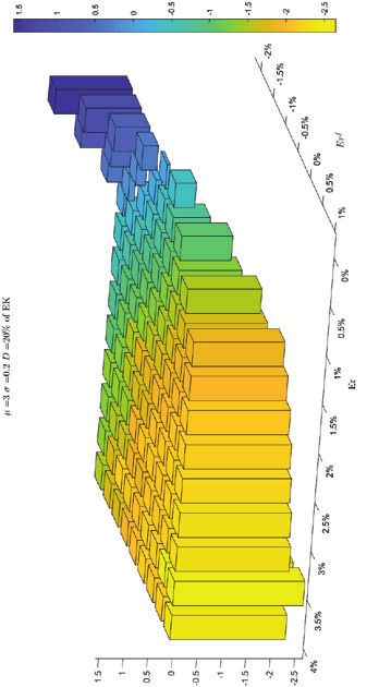
1198                                THE AMERICAN ECONOMIC REVIEW                                    APRIL 2019

                                                Introduction

   Since 1980, interest rates on US government bonds have steadily decreased. They
are now lower than the nominal growth rate, and according to current forecasts, this
is expected to remain the case for the foreseeable future. Ten-year US nominal rates
hover around 3 percent, while forecasts of nominal growth are around 4 percent (2
percent real growth, 2 percent inflation). The inequality holds even more strongly in
the other major advanced economies. The 10-year UK nominal rate is 1.3 percent,
compared to forecasts of 10-year nominal growth around 3.6 percent (1.6 percent
real, 2 percent inflation). The 10-year Euro nominal rate is 1.2 percent, compared to
forecasts of 10-year nominal growth around 3.2 percent (1.5 percent real, 1.7 percent
inflation).1 The 10-year Japanese nominal rate is 0.1 percent, compared to forecasts
of 10-year nominal growth around 1.4 percent (1.0 percent real, 0.4 percent inflation).
   The question I ask in this lecture is what the implications of such low rates should
be for government debt policy. It is an important question for at least two reasons.
From a policy viewpoint, whether or not countries should reduce their debt, and by
how much, is a central policy issue. From a theory viewpoint, one of the pillars of
macroeconomics is the assumption that people, firms, and governments are subject
to intertemporal budget constraints. If the interest rate paid by the government is less
than the growth rate, then the intertemporal budget constraint facing the government
no longer binds. What the government can and should do in this case is definitely
worth exploring.
   The paper reaches strong, and, I expect, surprising, conclusions. Put (too) simply,
the signal sent by low rates is not only that debt may not have a substantial fiscal
cost, but also that it may have limited welfare costs.
   Given that these conclusions are at odds with the widespread notion that gov-
ernment debt levels are much too high and must urgently be decreased, I consider
several counterarguments, ranging from distortions, to the possibility that the future
may be very different from the past, to multiple equilibria. All these arguments have
merit, but they imply a different discussion from that dominating current discus-
sions of fiscal policy.
   The lecture is organized as follows.
   Section I looks at the past behavior of US interest rates and growth rates. It con-
cludes that the current situation is actually not unusual. While interest rates on pub-
lic debt vary a lot, they have on average, and in most decades, been lower than
growth rates. If the future is like the past, the probability that the US government can
do a debt rollover, that it can issue debt and achieve a decreasing debt to GDP ratio
without ever having to raise taxes later, is high.
   That debt rollovers may be feasible does not imply however that they are desir-
able. Even if higher debt does not give rise later to a higher tax burden, it still has
effects on capital accumulation, and thus on welfare. Whether and when higher debt
increases or decreases welfare is taken up in Sections II and III.

    1
      Different Euro countries have different government bond rates. The 10-year Euro nominal rate is a composite
rate (with changing composition) constructed by the European Central Bank (ECB): http://sdw.ecb.europa.eu/
quickview.do?SERIES_KEY=143.FM.M.U2.EUR.4F.BB.U2_10Y.YLD.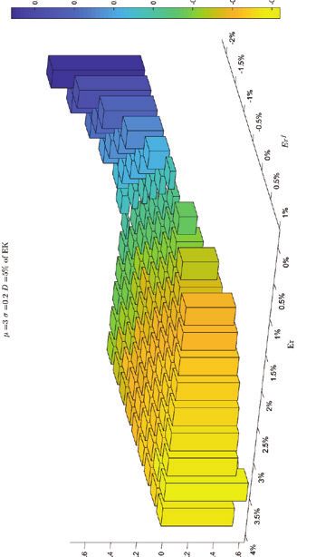
VOL. 109 NO. 4 BLANCHARD: PUBLIC DEBT AND LOW INTEREST RATES 1199
Section II looks at the effects of an intergenerational transfer (a conceptually sim-
pler policy than a debt rollover, but a policy that shows most clearly the relevant effects
at work) in an overlapping generation model with uncertainty. In the certainty context
analyzed by Diamond (1965), whether such an intergenerational transfer from young
to old is welfare improving depends on “the” interest rate, which in that model is sim-
ply the net marginal product of capital. If the interest rate is less than the growth rate,
then the transfer is welfare improving. Put simply, in that case, a larger intergenera-
tional transfer, or equivalently an increase in public debt, and thus less capital, is good.
When uncertainty is introduced however, the question becomes what interest rate
we should look at to assess the welfare effects of such a transfer. Should it be the
average safe rate, i.e., the rate on sovereign bonds (assuming no default risk), or
should it be the average marginal product of capital? The answer turns out to be: both.
As in the Diamond model, a transfer has two effects on welfare: an effect through
reduced capital accumulation, and an indirect effect, through the induced change in
the returns to labor and capital.
The welfare effect through lower capital accumulation depends on the safe rate.
It is positive if, on average, the safe rate is less than the growth rate. The intuitive
reason is that, in effect, the safe rate is the relevant risk-adjusted rate of return on
capital, thus it is the rate that must be compared to the growth rate.
The welfare effect through the induced change in returns to labor and capital
depends instead on the average (risky) marginal product of capital. It is negative if,
on average, the marginal product of capital exceeds the growth rate.
Thus, in the current situation where it indeed appears that the safe rate is less
than the growth rate, but the average marginal product of capital exceeds the growth
rate, the two effects have opposite signs, and the effect of the transfer on welfare
is ambiguous. The section ends with an approximation that shows most clearly the
relative role of the two rates. The net effect may be positive, if the safe rate is suffi-
ciently low and the average marginal product is not too high.
With these results in mind, Section III turns to numerical simulations. People live
for two periods, working in the first, and retiring in the second. They have separate
preferences vis-à-vis intertemporal substitution and risk. This allows to look at differ-
ent combinations of risky and safe rates, depending on the degree of uncertainty and
the degree of risk aversion. Production is constant elasticity of substitution (CES) in
labor and capital, and subject to technological shocks; being able to vary the elastic-
ity of substitution between capital and labor turns out to be important as this elasticity
determines the strength of the second effect on welfare. There is no technological
progress, nor population growth, so the average growth rate is equal to zero.
I show how the welfare effects of a transfer can be positive or negative, and how
they depend in particular on the elasticity of substitution between capital and labor.
In the case of a linear technology (equivalently, an infinite elasticity of substitution
between labor and capital), the rates of return, while random, are independent of
capital accumulation, so that only the first effect is at work, and the safe rate is the
only relevant rate in determining the effect of the transfer on welfare. I then show
how a lower elasticity of substitution implies a negative second effect, leading to an
ambiguous welfare outcome.
I then turn to debt and show that a debt rollover differs in two ways from a transfer
scheme. First, with respect to feasibility: so long as the safe rate remains less than the
1200 THE AMERICAN ECONOMIC REVIEW APRIL 2019
growth rate, the ratio of debt to GDP decreases over time; a sequence of adverse shocks
may however increase the safe rate sufficiently so as to lead to explosive dynamics,
with higher debt increasing the safe rate, and the higher safe rate in turn increasing
debt over time. Second, with respect to desirability: a successful debt rollover can yield
positive welfare effects, but less so than the transfer scheme. The reason is that a debt
rollover pays people a lower rate of return than the implicit rate in the transfer scheme.
The conclusion of Section III is that the welfare effects of debt depend not only on
how low the average safe rate is, but also on how high the average marginal product
is. With this in mind, Section IV returns to the empirical evidence on the marginal
product of capital, focusing on two facts. The first fact is that the ratio of the earnings
of US corporations to their capital at replacement cost has remained high and rela-
tively stable over time. This suggests a high marginal product, and thus, other things
equal, a higher welfare cost of debt. The second fact, however, is that the ratio of the
earnings of US corporations to their market value has substantially decreased since
the early 1980s. Put another way, Tobin’s q, which is the ratio of the market value of
capital to the value of capital at replacement cost, has substantially increased. There
are two potential interpretations of this fact. First, that capital at replacement cost
is poorly measured and does not fully capture intangible capital. Second, that an
increasing proportion of earnings comes from rents. Both explanations (which are
the subject of much current research) imply a lower marginal product for a given
measured earnings rate, and thus a smaller welfare cost of debt.
Section V goes beyond the formal model and places the results in a broader but
informal discussion of the costs and benefits of public debt.
On the benefit side, the model above has looked at debt issuance used to finance
transfers in a full employment economy; this does not do justice to current policy
discussions, which have focused on the role of debt finance to increase demand and
output if the economy is in recession, and on the use of debt to finance public invest-
ment. This research has concluded that, if the neutral rate of interest is low and the
effective lower bound on interest rates is binding, then there is a strong argument
for using fiscal policy to sustain demand. The analysis above suggests that, in that
very situation, the fiscal and welfare costs of higher debt may be lower than has been
assumed, reinforcing the case for a fiscal expansion.
On the cost side, (at least) three arguments can be raised against the model above
and its implications. The first is that the risk premium, and by implication the low
safe rate relative to the marginal product of capital, may not reflect risk preferences
but rather distortions, such as financial repression. Traditional financial repression,
i.e., forcing banks to hold government bonds, is gone in the United States, but one
may argue that agency issues within financial institutions or some forms of financial
regulation such as liquidity ratios have similar effects. The second argument is that
the future may be very different from the present, and the safe rate may turn out much
higher than in the past. The third argument is the possibility of multiple equilibria,
that if investors expect the government to be unable to fully repay the debt, they may
require a risk premium which makes debt harder to pay back and makes their expec-
tations self-fulfilling. I discuss all three arguments but focus mostly on the third. It is
relevant and correct as far as it goes, but it is not clear what it implies for the level of
public debt: multiple equilibria typically hold for a large range of debt, and a realistic
reduction in debt while debt remains in the range does not rule out the bad equilibrium.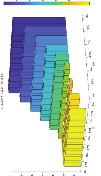
VOL. 109 NO. 4                  BLANCHARD: PUBLIC DEBT AND LOW INTEREST RATES                                  1201

   Section VI concludes. To be clear, the purpose of the lecture is not to advocate
for higher public debt, but to assess its costs. The hope is that this lecture leads to a
richer discussion of fiscal policy than is currently the case.

                      I. Interest Rates, Growth Rates, and Debt Rollovers

   Interest rates on US bonds have been and are still unusually low, reflecting in
part the after-effects of the 2008 financial crisis and quantitative easing. The current
(December 2018) 1-year T-bill nominal rate is 2.6 percent, substantially below the
most recent nominal growth rate, 4.8 percent (from 2018:II to 2018:III, at annual
rates).
   The gap between the two is expected to narrow, but most forecasts and market
signals have interest rates remaining below growth rates for a long time to come.
Despite a strong fiscal expansion putting pressure on rates in an economy close to
potential, the current 10-year nominal rate remains around 3 percent, while forecasts
of nominal growth over the same period are around 4 percent. Looking at real rates
instead, the current 10-year inflation-indexed rate is around 1 percent, while most
forecasts of real growth over the same period range from 1.5 percent to 2.5 percent.2
   These forecasts come with substantial uncertainty.
   Some argue that these low rates reflect “secular stagnation” forces that are likely
to remain relevant for the foreseeable future. They point to structurally high saving
and low investment, leading to a low equilibrium marginal product of capital for
a long time to come (for example, Summers 2015, Rachel and Summers 2018).
Others point to an increased demand for safe assets, leading to a lower safe rate for a
given marginal product (for example, Caballero, Farhi, and Gourinchas 2017a). An
interesting attempt to identify the respective roles of marginal products, rents, and
risk premia is given by Caballero, Farhi, and Gourinchas (2017b).
   Others point instead to factors such as aging in advanced economies, better social
insurance or lower reserve accumulation in emerging markets, which may lead
instead to higher rates in the future (for a discussion of the role of different factors,
see for example Rachel and Smith 2015, Lunsford and West 2018)3.
   Interestingly and importantly however, historically, interest rates lower than
growth rates have been more the rule than the exception, making the issue of what
debt policy should be under this configuration of more than temporary interest.
I shall limit myself here to looking at the United States since 1950, but the conclu-
sion holds for a large number of countries, over long periods of time.4

    2
      Since 1800, 10-year rolling sample averages of US real growth have always been positive, except for one
10-year period, centered in 1930.
    3
      Some have pointed to demographics as a factor likely to decrease the growth rate and increase the safe rate.
Theory and evidence however suggest a more complex answer. A decrease in fertility implies a decrease in both
the growth rate and the interest rate. An increase in longevity, unless accompanied by a proportional increase in
the retirement age, may have no effect on the growth rate but may lead to a decrease in the interest rate. Mehrotra
and Sergeyev (2018), using a calibrated overlapping generations (OLG) model, derive and discuss the effects of
population growth and productivity growth on the interest-growth rate differential. In current unpublished work,
Carvalho et al., extending Carvalho, Ferrero, and Nechio (2016) and also using a calibrated OLG model, conclude
that demographic evolutions are likely to lead to a lower neutral interest rate in the future.
    4
      Two major datasets are those put together by Shiller (1992 and updates) for the United States since 1871, and
by Jordà et al. (2017) for 16 countries since 1870. Based on these data, Mehrotra (2017) and Barrett (2018) show
that the safe rate has been typically lower on average than the growth rate. Mauro et al. (2015) look at the evidence
1202 THE AMERICAN ECONOMIC REVIEW APRIL 2019
16
14 1‐year T-bill rate
12 Nominal growth rate
10
8
6
4
2
0
−2
−4
19 0
1952
1954
1956
1958
1960
1962
1964
1966
1968
1970
1972
19 74
1976
1978
1980
1982
1984
1986
1988
1990
1992
1994
1996
2098
2000
2002
2004
2006
2008
2010
2012
2014
2016
18
5
19
Figure 1. Nominal GDP Growth Rate and 1-Year T-Bill Rate, 1950–2018
16
Nominal 10‐year rate
14
Nominal growth rate
12
10
8
6
4
2
0
−2
−4
19 0
1952
1954
1956
1958
1960
1962
1964
1966
1968
1970
1972
19 74
1976
1978
1980
1982
1984
1986
1988
1990
1992
1994
1996
2098
2000
2002
2004
2006
2008
2010
2012
2014
2016
18
5
19
Figure 2. Nominal GDP Growth Rate and 10-Year Bond Rate, 1950–2018
Figure 1 shows the evolution of the nominal GDP growth rate and the 1-year
Treasury bill rate. Figure 2 shows the evolution of the nominal GDP growth rate and
the 10-year Treasury bond rate. Together, they have two basic features:
• On average, over the period, nominal interest rates have been lower than the
nominal growth rate.5 The 1-year rate has averaged 4.7 percent, the 10-year rate
has averaged 5.6 percent, while nominal GDP growth has averaged 6.3 percent.6
• Both the 1-year rate and the 10-year rate were consistently below the growth
rate until the disinflation of the early 1980s. Since then, both nominal inter-
est rates and nominal growth rates have declined, with rates declining faster
than growth, even before the financial crisis. Overall, while nominal rates vary
from 55 countries since 1800. Their results, summarized in their Table 2, show that the safe interest rate has been
on average lower than the growth rate, both for the group of advanced countries, and for the group of non-advanced
economies. (For those who want to go back even further in time, data on the safe rate going back to the 14th century
have been put together by Schmelzing 2019 and show a steady decrease in the rate over 6 centuries.)
5
Equivalently, if one uses the same deflator, real interest rates have been lower than real growth rates. Real
interest rates are however often computed using CPI inflation rather than the GDP deflator.
6
Using Shiller’s numbers for interest rates and historical BEA series for GDP, over the longer period 1871 to
2018, the 1-year rate has averaged 4.6 percent, the 10-year rate 4.6 percent, and nominal GDP growth 5.3 percent.VOL. 109 NO. 4 BLANCHARD: PUBLIC DEBT AND LOW INTEREST RATES 1203
s ubstantially from year to year, the 1-year rate has been lower than the growth
rate for all decades except for the 1980s. The 10-year rate has been lower than
the growth rate for 4 out of 7 decades.
Given that my focus is on the implications of the joint evolution of interest rates
and growth rates for debt dynamics, the next step is to construct a series for the rele-
vant interest rate paid on public debt held by domestic private and foreign investors.
I proceed in three steps, (i) taking into account the maturity composition of the debt,
(ii) taking into account the tax payments on the interest received by the holders of
public debt, and (iii) taking into account Jensen’s inequality. (Details of construc-
tion are given in online Appendix A.)7
To take into account maturity, I use information on the average maturity of the
debt held by private investors (that is excluding public institutions and the Fed).
This average maturity went down from eight years and four months in 1950 to three
years and four months in 1974, with a mild increase since then to five years today.8
Given this series, I construct a maturity-weighted interest rate as a weighted aver-
age of the 1-year and the 10-year rates using it = αt × i1,t + (1 − αt) × i10,t with
αt = (10 − average maturity in years)/9.
Many, but not all, holders of government bonds pay taxes on the interest paid,
so the interest cost of debt is actually lower than the interest rate itself. There is no
direct measure of those taxes, and thus I proceed as follows.9,10
I measure the tax rate of the marginal holder by looking at the difference between
the yield on AAA municipal bonds (which are exempt from federal taxes) and
the yield on a corresponding maturity Treasury bond, for both 1-year and 10-year
bonds, denoted im t1and im t10respectively. Assuming that the marginal investor is
indifferent between holding the 2, the implicit tax rate on 1-year Treasuries is given
by τ1t = 1 − imt1/i1t, and the implicit tax rate on 10-year Treasuries is given by
τ10t = 1 − imt10/i10t.11 The tax rate on 1-year bonds peaks at about 50 percent in
the late 1970s (as inflation and nominal rates are high, leading to high effective tax
rates), then goes down close to 0 until the financial crisis, and has increased slightly
since 2017. The tax rate on 10-year bonds follows a similar pattern, down from
about 40 percent in the early 1980s to close to 0 until the financial crisis, with a
small increase since 2016.12 Taking into account the maturity structure of the debt,
I then construct an average tax rate in the same way as I constructed the interest rate
above, by constructing τt = αt × τ1,t + (1 − αt) × τ10,t
.
7
A more detailed construction of the maturity of the debt held by both private domestic and foreign investors is
given in Hilscher, Raviv, and Reis (2018).
8
Fed holdings used to be small, and limited to short maturity T-bills. As a result of quantitative easing, they have
become larger and skewed toward long maturity bonds, implying a lower maturity of debt held by private investors
than of total debt.
9
For a parallel study, see Feenberg, Tepper, and Welch (2018).
10
This is clearly only a partial equilibrium computation. To the extent that debt leads to lower capital accumu-
lation and thus lower output, other tax revenues may decrease. To the extent however that consumption decreases
less or even increases (as discussed in the next section), the effects depend on how much of taxation is output based
or consumption based.
11
This is an approximation. On the one hand, the average tax rate is likely to exceed this marginal rate. On the
other hand, to the extent that municipal bonds are also partially exempt from state taxes, the marginal tax rate may
reflect in part the state tax rate in addition to the Federal tax rate.
12
The computed tax rates are actually negative during some of the years of the Great Recession, presumably
reflecting the effects of Quantitative Easing. I put them equal to zero for those years.1204 THE AMERICAN ECONOMIC REVIEW APRIL 2019
16
14 10‐year rate
12 1‐year rate
10 Adjusted rate
8
6
4
2
0
19 0
1952
1954
1956
1958
1960
1962
1964
1966
1968
1970
1972
19 74
1976
1978
1980
1982
1984
1986
1988
1990
1992
1994
1996
2098
2000
2002
2004
2006
2008
2010
2012
2014
2016
18
5
19
Figure 3. 1-Year Rate, 10-Year Rate, and Adjusted Rate, 1950–2018
16
14 Adjusted rate
12 Nominal GDP growth
10
8
6
4
2
0
−2
−4
1952
1954
1956
1958
1960
1962
1964
1966
1968
1970
1972
19 74
1976
1978
1980
1982
1984
1986
1988
1990
1992
1994
1996
2098
2000
2002
2004
2006
2008
2010
2012
2014
2016
18
19
Figure 4. Nominal GDP Growth Rate and Adjusted Rate, 1950–2018
Not all holders of Treasuries pay taxes however. Foreign holders, private and
public (such as central banks), Federal retirement programs, and Fed holdings are
not subject to tax. The proportion of such holders has steadily increased over time,
reflecting the increase in emerging markets’ reserves (in particular China’s), the
growth of the Social Security Trust Fund, and more recently, the increased holdings
of the Fed, among other factors. From 15 percent in 1950, it now accounts for 64
percent today.
Using the maturity adjusted interest rate from above, it, the implicit tax rate,
τt, and the proportion of holders likely subject to tax, β
t, I construct an “adjusted
interest rate” series according to
iadj,t = it( 1 − τt × βt) .
Its characteristics are shown in Figures 3 and 4. Figure 3 plots the adjusted rate
against the 1-year and the 10-year rates. Figure 4 plots the adjusted tax rate against
the nominal growth rate. They yield two conclusions:
• First, over the period, the average adjusted rate has been lower than either the
1-year or the 10-year rates, averaging 3.8 percent since 1950. This howeverVOL. 109 NO. 4 BLANCHARD: PUBLIC DEBT AND LOW INTEREST RATES 1205
largely reflects the nonneutrality of taxation to inflation in the 1970s and 1980s,
which is much less of a factor today. In 2018, the rate was around 2.4 percent.
• Second, over the period, the average adjusted rate has been substantially lower
than the average nominal growth rate, 3.8 percent versus 6.3 percent.
The last potential issue is Jensen’s inequality. The dynamics of the ratio of debt
to GDP are given by
1 + radj,t
dt = _
d + xt,
1 + gt t−1
where dtis the ratio of debt to GDP (with both variables either in nominal or in real
terms if both are deflated by the same deflator), and x tis the ratio of the primary
deficit to GDP (again, with both variables either in nominal or in real terms). The
evolution of the ratio depends on the relevant product of interest rates and growth
rates (nominal or real) over time.
Given the focus on debt rollovers, that is, the issuance of debt without a
later increase in taxes or reduction in spending, suppose we want to trace debt
dynamics under the assumption that xtremains equal to zero.13 Suppose that
ln[( 1 + radj,t) /( 1 + gt) ]is distributed normally with mean μand variance σ 2. Then,
the evolution of the ratio will depend not on exp μbut on exp(μ + (1/2) σ 2). We
have seen that, historically, μwas between −1 percent and −2 percent. The standard
deviation of the log ratio over the same sample is equal to 2.8 percent, implying
a variance of 0.08 percent, thus too small to affect the conclusions substantially.
Jensen’s inequality is thus not an issue here.14
In short, if we assume that the future will be like the past (admittedly a big if),
debt rollovers appear feasible. While the debt ratio may increase for some time due
to adverse shocks to growth or positive shocks to the interest rate, it will eventually
decrease over time. In other words, higher debt may not imply a higher fiscal cost.
In this light, it is interesting to do the following counterfactual exercise.15 Assume
that the debt ratio in year t was what it actually was, but that the primary balance was
equal to zero from then on, so that debt in year t + nwas given by
n 1 + radj,t+i
(i=1 1 + gt+i ) t
dt+n = ∏ _
d.
Figures 5 and 6 show what the evolution of the debt ratio would have been, start-
ing at different dates in the past. For convenience, the ratio is normalized to 100 at
each starting date. Figure 5 uses the non-tax adjusted rate, and Figure 6 uses the
tax-adjusted interest rate.
Figure 5 shows that, for each starting date, the debt ratio would eventually have
decreased, even in the absence of a primary surplus. The decrease, if starting in the
13
Given that we subtract taxes on interest from interest payments, the primary balance must also be computed
subtracting those tax payments.
14
The conclusion is the same if we do not assume log normality, but rather bootstrap from the actual distribu-
tion, which has slightly fatter tails.
15
For related computations and related conclusions, see Mehrotra and Sergeyev (2018).1206 THE AMERICAN ECONOMIC REVIEW APRIL 2019
140
120
100
Index
80
60
40
1950 1960 1970 1980 1990 2000 2010 2020
Figure 5. Debt Dynamics, with Zero Primary Balance, Starting in Year t, Using the Non-Tax Adjusted
Rate
100
80
Index
60
40
20
1950 1960 1970 1980 1990 2000 2010 2020
Figure 6. Debt Dynamics, with Zero Primary Balance, Starting in Year t, Using the Tax-Adjusted Rate
1950s, 1960s, or 1970s, is quite dramatic. But the figure also shows that a series
of bad shocks, such as happened in the 1980s, can increase the debt ratio to higher
levels for a while.
Figure 6, which I believe is the more appropriate one, gives an even more optimis-
tic picture, where the debt ratio rarely would have increased, even in the 1980s: the
reason being the higher tax revenues associated with inflation during that period.
What these figures show is that, historically, debt rollovers would have been fea-
sible. Put another way, it shows that the fiscal cost of higher debt would have been
small, if not zero. This is at striking variance with the current discussions of fiscal
space, which all start from the premise that the interest rate is higher than the growth
rate, implying a tax burden of the debt.
The fact that debt rollovers may be feasible (i.e., that they may not have a fiscal
cost) does not imply however that they are desirable (that they have no welfare cost).
This is the topic taken up in the next two sections.VOL. 109 NO. 4 BLANCHARD: PUBLIC DEBT AND LOW INTEREST RATES 1207
II. Intergenerational Transfers and Welfare
Debt rollovers are, by their nature, non-steady-state phenomena, and have poten-
tially complex dynamics and welfare effects. It is useful to start by looking at a sim-
pler policy, namely a transfer from the young to the old (equivalent to pay-as-you-go
social security), and then to return to debt and debt rollovers in the next section.
The natural setup to explore the issues is an overlapping generation model under
uncertainty. The overlapping generation structure implies a real effect of intergen-
erational transfers or debt, and the presence of uncertainty allows to distinguish
between the safe rate and the risky marginal product of capital.16
I proceed in two steps, first briefly reviewing the effects of a transfer under
certainty, following Diamond (1965), then extending it to allow for uncertainty.
(Derivations are given in online Appendix B.)17,18
Assume that the economy is populated by people who live for two periods, work-
ing in the first period, and consuming in both periods. Their utility is given by
U = (1 − β)U( C1) + βU(C2),
where C1and C2are consumption in the first and the second period of life, respec-
tively. (As I limit myself for the moment to looking at the effects of the transfer
on utility in steady state, there is no need for now for a time index.) Their first and
second period budget constraints are given by
C1 = W − K − D;
C2 = RK + D,
where Wis the wage, Kis saving (equivalently, next period capital), Dis the transfer
from young to old, and Ris the rate of return on capital.
I ignore population growth and technological progress, so the growth rate is equal
to zero. Production is given by a constant returns production function,
Y = F(K, N).
It is convenient to normalize labor to 1, so Y = F(K, 1). Both factors are paid
their marginal product.
16
In this framework, the main general equilibrium effect of intergenerational transfers or debt is to decrease
capital accumulation. A number of recent papers have explored the effects of public debt when public debt also
provides liquidity services. Aiyagari and McGrattan (1998) for example explore the effects of public debt in an
economy in which agents cannot borrow and thus engage in precautionary saving; in that framework, debt relaxes
the borrowing constraint and decreases capital accumulation. Angeletos, Collard, and Dellas (2016) develop a
model where public debt provides liquidity. In that model, debt can either crowd out capital, for the same reasons as
in Aiyagari and McGrattan, or crowd in capital by increasing the available collateral required for investment. These
models are obviously very different from the model presented here, but they share a focus on the low safe rate as
a signal about the desirability of public debt. Finally, to the extent that it focuses on economies where the safe rate
may be less than the growth rate, it is related to the literature on rational bubbles in dynamically efficient economies
with financial frictions, for example Martin and Ventura (2016), or Farhi and Tirole (2012).
17
For a nice introduction to the logic and implications of the overlapping generation model, see Weil (2008).
18
After the lecture was delivered, I was made aware of unpublished notes by Waldman (2016), which explore a
closely related model under different forms of uncertainty and also show that the welfare effects of debt depend in
general on both the safe and the risky rate.1208 THE AMERICAN ECONOMIC REVIEW APRIL 2019
The first-order condition for utility maximization is given by
(1 − β)U′(C1) = βRU′(C2) .
The effect of a small increase in the transfer D
on utility is given by
dU = [− (1 − β)U′(C1) + βU′(C2)]dD + [(1 − β)U′(C1)dW + βKU′(C2)dR].
The first term in brackets, call it d Ua, represents the partial equilibrium, direct,
effect of the transfer. The second term, call it d Ub, represents the general equilibrium
effect of the transfer through the induced change in wages and rates of return.
Consider the first term, the effect of debt on utility given labor and capital prices.
Using the first-order condition gives
dUa = [β(− RU′(C2) + U′(C2))]dD = β(1 − R)U′(C2) dD.
(1)
< 1 (the case known as “dynamic inefficiency”), then, ignoring the
So, if R
other term, a small increase in the transfer increases welfare. The explanation is
< 1, the transfer gives a higher rate of return to savers than
straightforward. If R
does capital.
Take the second term, the effect of debt on utility through the changes in W
and
R. An increase in debt decreases capital and thus decreases the wage and increases
the rate of return on capital. What is the effect on welfare?
Using the factor price frontier relation dW/dR = −K/N, or equivalently
dW = −K dR (given that N = 1), rewrite this second term as
dUb = − [( 1 − β)U′(C1) − βU′(C2)]K dR.
Using the first-order condition for utility maximization gives
dUb = − [β(R − 1)U′(C2)]K dR.
< 1then, just like the first term, a small increase in the transfer increases
So, if R
welfare (as the lower capital stock leads to an increase in the interest rate). The
explanation is again straightforward: given the factor price frontier relation, the
decrease in the capital leads to an equal decrease in income in the first period and
increase in income in the second period. If R < 1, this is more attractive than what
capital provides, and thus increases welfare.
Using the definition of the elasticity of substitution η ≡ (FK FN ) /FKNF, the defi-
nition of the share of labor, α = FN /F, and the relation between second derivatives
of the production function, FNK = − KFKK , this second term can be rewritten as
dUb = [β(1/η)α][(R − 1)U′(C2)]R dK.
(2) VOL. 109 NO. 4 BLANCHARD: PUBLIC DEBT AND LOW INTEREST RATES 1209
Note the following two implications of equations (1) and (2):
• The sign of the two effects depends on R − 1. If R
< 1, then a decrease in
capital accumulation increases utility. In other words, if the marginal product is
less than the growth rate (which here is equal to 0), an intergenerational transfer
has a positive effect on welfare in steady state.
• The strength of the second effect depends on the elasticity of substitution η. If
for example η = ∞so the production function is linear and capital accumula-
tion has no effect on either wages or rates of return to capital, this second effect
is equal to 0.
So far, I just replicated the analysis in Diamond.19 Now I introduce uncertainty in
production, so the marginal product of capital is uncertain. If people are risk averse,
the average safe rate will be less than the average marginal product of capital. The
basic question becomes: what is the relevant rate we should look at for welfare pur-
poses? Put loosely, is it the average marginal product of capital ER, or is it the average
safe rate ER f, or is it some other rate altogether?
The model is the same as before, except for the introduction of uncertainty.
People born at time thave expected utility given by (I now need time subscripts
as the steady state is stochastic)
Ut ≡ (1 − β)U( C1,t) + βEU(C2,t+1).
Their budget constraints are given by
C1t = Wt − Kt − D;
C2t+1 = Rt+1Kt + D.
Production is given by a constant returns production function
Yt = At F(Kt−1, N),
where N = 1and Atis stochastic. (The capital at time treflects the saving of the
young at time t − 1, thus the timing convention.)
At time t, the first-order condition for utility maximization is given by
(1 − β)U′(C1,t
) = βE[Rt+1
U′(C2,t+1
)].
We can now define a shadow safe rate R ft+1, which must satisfy
R ft+1 E[U′(C2,t+1
) ] = E[Rt+1
U′(C2,t+1)].
19
Formally, Diamond looks at the effects of a change in debt rather than a transfer. But, under certainty and in
steady state, the two are equivalent.1210 THE AMERICAN ECONOMIC REVIEW APRIL 2019
Now consider a small increase in D
on utility at time t:
dUt = [− (1 − β)U′(C1,t) + βEU′(C2,t+1
)]dD
+ [(1 − β)U′(C1,t
) dWt + βKt E[U′(C2,t+1
) dRt+1
]].
As before, the first term in brackets, call it dUat, reflects the partial equilibrium,
direct, effect of the transfer, the second term, call it dUbt, reflects the general equilib-
rium effect of the transfer through the change in wages and rates of return to capital.
Take the first term, the effect of debt on utility given prices. Using the first-order
condition gives
dUat = [− βE[Rt+1U′(C2,t+1)] + βE[U′(C2,t+1)]] dD.
So, using the definition of the safe rate:
dUat = β(1 − R ft+1) EU′(C2,t+1)dD.
(3)
So, to determine the sign effect of the transfer on welfare through this first chan-
nel, the relevant rate is indeed the safe rate. In any period in which R ft+1is less than
1, the transfer is welfare improving.
The reason why the safe rate is what matters is straightforward and important:
the safe rate is, in effect, the risk-adjusted rate of return on capital.20 The intergen-
erational transfer gives people a higher rate of return than the risk-adjusted rate of
return on capital.
Take the second term, the effect of the transfer on utility through prices:
dUbt = (1 − β)U′(C1,t) dWt + βE[U′(C2,t+1)Kt dRt+1].
Or using the factor price frontier relation:
dUbt = (−1 − β)U′(C1,t) Kt−1 dRt + βE[U′(C2,t+1)Kt dRt+1].
In general, this term will depend both on d Kt−1 (which affects d Wt) and on dKt
(which affects dRt+1). If we evaluate it at K
t = Kt−1 = Kand dKt = dKt+1
= dK, it can be rewritten, using the same steps as in the certainty case, as
Rt+1
[ t ) ( 2,t+1)] t
dUbt = [β(1/η)α]E (Rt+1
(4) − _ U′ C R dK,
R
or
(5) dUbt = [β(1/η)α]E[ Rt+1U′(C2,t+1)](Rt − 1) dK.
Thus, the relevant rate in assessing the sign of the welfare effect of the transfer
t is
through this second term is the risky rate, the marginal product of capital. If R
20
The relevance of the safe rate in assessing the return to capital accumulation was one of the themes in
Summers (1990).VOL. 109 NO. 4 BLANCHARD: PUBLIC DEBT AND LOW INTEREST RATES 1211
less than 1, the implicit transfer due to the change in input prices increases utility. If
Rtis greater than 1, the implicit transfer decreases utility.
The reason why it is the risky rate that matters is simple. Capital yields a rate of
return Rt+1. The change in prices due to the decrease in capital represents an implicit
transfer with rate of return Rt+1/Rt. Thus, whether the implicit transfer increases or
decreases utility depends on whether R tis less or greater than 1.
Putting the two sets of results together: if the safe rate is less than 1, and
the risky rate is greater than 1 (the configuration that appears to be relevant
today) the two terms now work in opposite directions. The first term implies that an
increase in debt increases welfare. The second term implies that an increase in debt
instead decreases welfare. Both rates are thus relevant.
To get a sense of relative magnitudes of the two effects, and therefore which one
is likely to dominate, the following approximation is useful. Evaluate the two terms
at the average values of the safe and the risky rates, to get
[(1 − ER ) − (1/η)α ER (ER − 1)(− dK/dD)]βE[U′(C2)]
dU/dD = f f
so that
(6) sign dU ≡ sign[(1 − ER f ) − (1/η)αER f(− dK/dD)(ER − 1)]
where, from the accumulation equation, we have the following approximation:21
dK/dD ≈ − ___________
1 .
1 − βα(1/η)ER
Note that, if the production is linear, and so η = ∞, the second term in equation
(6) is equal to 0, and the only rate that matters is E R f. Thus, if ER fis less than 1, a
higher transfer increases welfare. As the elasticity of substitution becomes smaller,
the price effect becomes stronger, and, eventually, the welfare effect changes sign
and becomes negative.
In the Cobb-Douglas case, using the fact that E R ≈ (1 − α)/( αβ), (the approx-
imation comes from ignoring Jensen’s inequality) the equation reduces to the sim-
pler formula:
(7) sign dU ≡ sign[(1 − ER f ER)].
Suppose that the average annual safe rate is 2 percent lower than the growth rate,
R f, the gross rate of return over a unit period, say 25 years, is 0 .98 25 = 0.6,
so that E
then the welfare effect of a small increase in the transfer is positive if E Ris less than
1.66, or equivalently, if the average annual marginal product is less than 2 percent
above the growth rate.22
21
This is an approximation in two ways. It ignores uncertainty and assumes that the direct effect of the transfer
on saving is one for one, which is an approximation.
22
Note that the economy we are looking at may be dynamically efficient in the sense of Zilcha (1991). Zilcha
defined dynamic efficiency as the condition that there is no reallocation such that consumption of either the young
or the old can be increased in at least one state of nature and one period, and not decreased in any other; the motiva-
tion for the definition is that it makes the condition independent of preferences. He then showed that in a stationary1212 THE AMERICAN ECONOMIC REVIEW APRIL 2019
Short of a much richer model, it is difficult to know how reliable these rough
computations are as a guide to reality. The model surely overstates the degree of
non-Ricardian equivalence: debt in this economy is (nearly fully) net wealth, even
if R fis greater than 1 and the government must levy taxes to pay the interest to keep
the debt constant. The assumption that capital and labor are equally risky may not
be right: holding claims to capital (i.e., shares) involves price risk, which is absent
from the model as capital fully depreciates within a period; on the other hand, labor
income, in the absence of insurance against unemployment, can also be very risky.
Another restrictive assumption of the model is that the economy is closed: in an
open economy, the effect on capital is likely to be smaller, with changes in public
debt being partly reflected in increases in external debt. I return to the issue when
discussing debt (rather than intertemporal transfers) later. Be this as it may, the anal-
ysis suggests that the welfare effects of a transfer may not necessarily be adverse, or,
if adverse, may not be very large.
III. Simulations: Transfers, Debt, and Debt Rollovers
To get a more concrete picture, and turn to the effects of debt and debt rollovers
requires going to simulations.23 Within the structure of the model above, I make the
following specific assumptions (derivations and details of simulations are given in
online Appendix C).
I think of each of the two periods of life as equal to 25 years. Given the role of
risk aversion in determining the gap between the average safe and risky rates, I want
to separate the elasticity of substitution across the two periods of life and the degree
of risk aversion. Thus, I assume that utility has an Epstein-Zin-Weil representation
of the form (Epstein and Zin 2013, Weil 1990):
(1 − β)ln C1,t + β _
( 2,t+1)
1 ln E C 1−γ .
1−γ
The log-log specification implies that the intertemporal elasticity of substitution
is equal to 1. The coefficient of relative risk aversion is given by γ.
As the strength of the second effect above depends on the elasticity of substitution
between capital and labor, I assume that production is characterized by a c onstant
elasticity of substitution production function, with multiplicative uncertainty:
Yt = At (bK ρt−1 +
(1 − b) N ρ) = At (bK ρt−1 +
(1 − b))
1/ρ 1/ρ
,
where Atis white noise and is distributed log normally, with ln At ∼ (μ; σ 2) and
ρ = (η − 1)/η, where ηis the elasticity of substitution. When η = ∞, ρ = 1 and
the production function is linear.
economy, a necessary and sufficient condition for dynamic inefficiency is that E ln R > 0. What the argument in the
text has shown is that an intergenerational transfer can be welfare improving even if the Zilcha condition holds. As
we saw, expected utility can increase even if the average risky rate is large, so long as the safe rate is low enough.
The reallocation is such that consumption indeed decreases in some states, yet expected utility is increased.
23
One can make some progress analytically, and, in Blanchard and Weil (2001), we did characterize the behav-
ior of debt at the margin (that is, taking the no-debt prices as given), for a number of different utility and production
functions and different incomplete market structures. We only focused on debt dynamics however, and not on the
normative implications.VOL. 109 NO. 4 BLANCHARD: PUBLIC DEBT AND LOW INTEREST RATES 1213
Finally, I assume that, in addition to the wage, the young receive a nonstochastic
endowment, X. Given that the wage follows a log normal distribution and thus can
be arbitrarily small, such an endowment is needed to make sure that the determin-
istic transfer from the young to the old is always feasible, no matter what the real-
ization of W.24 I assume that the endowment is equal to 100 percent of the average
wage absent the transfer.
Given the results in the previous section, I calibrate the model so as to fit a set
of values for the average safe rate and the average risky rate. I consider average net
annual risky rates (marginal products of capital) minus the growth rate (here equal
to 0) between 0 percent and 4 percent. These imply values of the average 25-year
gross risky rate, ER, between 1.00 and 2.66. I consider average net annual safe rates
minus the growth rate between −2 percent and 1 percent; these imply values of the
average 25-year gross safe rate, E R f, between 0.60 and 1.28.
I choose some of the coefficients a priori. I choose b (which is equal to the capital
share in the Cobb-Douglas case) to be 1/3. For reasons explained below, I choose
the_annual value of σato be a high 4 percent a year, which implies a value of σ of
√25 × 4% = 0.20.
Because the strength of the second effect above depends on the elasticity of sub-
stitution, I consider two different values of η, η = ∞which corresponds to the
linear production function case, and in which the price effects of lower capital accu-
mulation are equal to 0, and η = 1, the Cobb-Douglas case, which is generally seen
as a good description of the production function in the medium run.
The central parameters are, on the one hand, β and μ, and on the other, γ.
The parameters β and μ determine (together with σ , which plays a minor role)
the average level of capital accumulation and thus the average marginal product of
capital: i.e., the average risky rate. In general, both parameters matter. In the linear
production case however, the marginal product of capital is independent of the level
of capital, and depends only on μ; thus, I choose μ to fit the average value of the
marginal product E R. In the Cobb-Douglas case, the marginal product of capital is
instead independent of μ and depends only on β; thus, I choose βto fit the average
value of the marginal product ER.
The parameter γ determines, together with σ , the spread between the risky rate
and the safe rate. In the absence of transfers, the following relation holds between
the two rates:
ln R ft+1 − ln ERt+1
= − γσ 2.
This relation implies however that the model suffers from a strong case of the
equity premium puzzle (see, for example, Kocherlakota 1996). If we think of σ as
the standard deviation of TFP growth, and assume that, in the data, TFP growth is
a random walk (with drift), this implies an annual value of σ aof about 2 percent,
equivalently a value of σover the 25-year period of 10 percent, and thus a value of
σ 2of 1 percent. Thus, if we think of the annual risk premium as equal to, say, 5 per-
cent, which implies a value of the right-hand side of 1.22, this implies a value of γ,
24
Alternatively, a lower bound on the wage distribution will work as well. But this would imply choosing an
other distribution than the log normal.1214 THE AMERICAN ECONOMIC REVIEW APRIL 2019
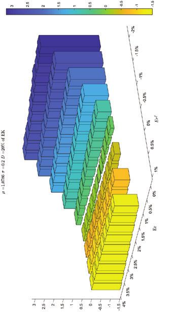
Mean utility, linear production with aggregate risk
= 1.0786, σ = 0.2, D = 5% of EK
3%
2.5%
2%
0.8
1.5%
0.6
1%
0.4
0.5%
0.2 0%
0 −0.5%
−0.2 −1%
−1.5%
−1.5% −2%
4% 3.5%
−0.5%−1%
3% 2.5% 2%
1.5% 1% 0.5% 0% 1% 0.5% 0%
ER ER
Figure 7. Welfare Effects of a Transfer of 5 Percent of Saving (Linear Production Function)
the coefficient of relative risk aversion of 122, which is clearly implausible. One of
the reasons why the model fails so badly is the symmetry in the degree of uncer-
tainty facing labor and capital, and the absence of price risk associated with holding
shares (as capital fully depreciates within the 25-year period). If we take instead σ to
reflect the standard deviation of annual rates of stock returns, say 15 percent a year
(its historical mean), and assume stock returns to be uncorrelated over time, then
σover the 25-year period is equal to 75 percent, implying values of γ around 2.5.
There is no satisfactory way to deal with the issue within the model, so as an uneasy
compromise, I choose σ = 20%. Given σ, γ is determined for each pair of average
risky and safe rates.25
I then consider the effects on steady-state welfare of an intergenerational transfer.
The basic results are summarized in Figures 7 to 10.
Figure 7 shows the effects of a small transfer (5 percent of (pre-transfer) average
saving) on welfare for the different combinations of the safe and the risky rates
(reported, for convenience, as net rates at annual values, rather than as gross rates
at 25-year values), in the case where η = ∞and, thus, production is linear. In this
case, the derivation above showed that, to a first order, only the safe rate mattered.
This is confirmed visually in the figure. Welfare increases if the safe rate is negative
(more precisely, if it is below the growth rate, here equal to 0), no matter what the
average risky rate.
Figure 8 looks at a larger transfer (20 percent of saving), again in the linear
production case. For a given ER f, a larger ERleads to a smaller welfare increase if
welfare increases, and to a larger welfare decrease if welfare decreases. The reason
is as follows. As the size of the transfer increases, second period income becomes
less risky, so the risk premium decreases, increasing ER ffor given average ER. In
25
Extending the model to allow uncertainty to differ for capital and labor is difficult to do (except for the case
where production is linear and one can easily capture capital or labor augmenting technology shocks).VOL. 109 NO. 4 BLANCHARD: PUBLIC DEBT AND LOW INTEREST RATES 1215
Mean utility, linear production with aggregate risk
= 1.0786, σ = 0.2, D = 20% of EK
3%
2.5%
3%
2.5% 2%
2%
1.5%
1.5%
1% 1%
0.5%
0% 0.5%
−0.5%
0%
−1%
−1.5% −0.5%
4%
3.5% 3%
2.5% 2% −1.5% −2% −1%
−1%
0% −0.5%
1.5%
1%
0.5% 0% 0.5% −1.5%
ER 1% ER f
Figure 8. Welfare Effects of a Transfer of 20 Percent of Saving (Linear Production Function)
the limit, a transfer that led people to save nothing in the form of capital would elim-
inate uncertainty about second period income, and thus would lead to E R f = ER.
The larger ER, the faster ER increases with a large transfer; for ERhigh enough ,
f
and for Dlarge enough, ER fbecomes larger than 1, and the transfer becomes welfare
decreasing.
In other words, even if the transfer has no effect on the average rate of return to
capital, it reduces the risk premium, and thus increases the safe rate. At some point,
the safe rate becomes positive, and the transfer has a negative effect on welfare.
Figures 9 and 10 do the same, but now for the Cobb-Douglas case. They yield
the following conclusions. Both effects are now at work, and both rates matter. A
lower safe rate makes it more likely that the transfer will increase welfare; a higher
risky rate makes it less likely. For a small transfer (5 percent of saving), a safe rate
2 percent lower than the growth rate leads to an increase in welfare so long as the
risky rate is less than 2 percent above the growth rate. A safe rate 1 percent lower
than the growth rate leads to an increase in welfare so long as the risky rate is less
than 1 percent above the growth rate. For a larger transfer (20 percent of saving),
which increases the average R fcloser to 1, the trade-off becomes less attractive. For
welfare to increase, a safe rate 2 percent lower than the growth rate requires that
the risky rate be less than 1.5 percent above the growth rate; a safe rate of 1 percent
below the growth rate requires that the risky rate be less than 0.7 percent above the
growth rate.
I have so far focused on intergenerational transfers, such as we might observe in
a pay-as-you-go system. Building on this analysis, I now turn to debt, and proceed
in two steps, looking first at the effects of a permanent increase in debt, then looking
at debt rollovers.
Suppose the government increases the level of debt and maintains it at this higher
level forever. Depending on the value of the safe rate every period, this may require
either issuing new debt when R ft < 1and distributing the proceeds as benefits, or
retiring debt, when R ft > 1and financing it through taxes. Following Diamond,You can also read