Marginalized Stochastic Natural Gradients for Black-Box Variational Inference
←
→
Page content transcription
If your browser does not render page correctly, please read the page content below

Marginalized Stochastic Natural Gradients for Black-Box Variational Inference

                                     Geng Ji 1 2 Debora Sujono 2 Erik B. Sudderth 2

                         Abstract                                 update single (or small blocks of) variational parameters,
                                                                  while holding all others fixed to their current values. Al-
     Black-box variational inference algorithms use               though CAVI updates can be effective for simple models
     stochastic sampling to analyze diverse statisti-             composed from conjugate priors, for many models the ex-
     cal models, like those expressed in probabilistic            pectations required for exact CAVI updates are intractable:
     programming languages, without model-specific                they may require complex integrals for continuous variables,
     derivations. While the popular score-function es-            or computation scaling exponentially with the number of
     timator computes unbiased gradient estimates, its            dependent discrete variables.
     variance is often unacceptably large, especially in
     models with discrete latent variables. We propose            Variational algorithms for models with non-conjugate con-
     a stochastic natural gradient estimator that is as           ditionals have been derived via hand-crafted auxiliary vari-
     broadly applicable and unbiased, but improves                ables that induce looser, but more tractable, bounds on the
     efficiency by exploiting the curvature of the vari-          data log-likelihood (Jordan et al., 1999; Winn & Bishop,
     ational bound, and provably reduces variance                 2005). Such bounds typically require complex derivations
     by marginalizing discrete latent variables. Our              specialized to the parametric structure of specific distri-
     marginalized stochastic natural gradients have in-           butions (Albert & Chib, 1993; Jaakkola & Jordan, 1999;
     triguing connections to classic coordinate ascent            Polson et al., 2013), and thus do not easily integrate with
     variational inference, but allow parallel updates            general-purpose probabilistic inference systems.
     of variational parameters, and provide superior              To address these limitations, several authors have explored
     convergence guarantees relative to naive Monte               stochastic gradient algorithms that directly optimize a repa-
     Carlo approximations. We integrate our method                rameterized bound involving the log-likelihood gradient
     with the probabilistic programming language Pyro             or score function (Paisley et al., 2012; Wingate & Weber,
     and evaluate real-world models of documents, im-             2013; Ranganath et al., 2014), as in the classic REINFORCE
     ages, networks, and crowd-sourcing. Compared                 policy gradient algorithm (Williams, 1992). Unlike other
     to score-function estimators, we require far fewer           black-box variational methods such as automatic differenti-
     Monte Carlo samples and consistently conver-                 ation variational inference (ADVI, Kucukelbir et al. (2017))
     gence orders of magnitude faster.                            that require specific variable reparameterizations (Kingma
                                                                  & Welling, 2014; Rezende et al., 2014), REINFORCE pro-
                                                                  vides unbiased gradients for all models including the many
1. Introduction                                                   practically important ones with discrete latent variables.
Variational inference is widely used to estimate the poste-       Due to its simplicity and generality, REINFORCE has be-
rior distributions of hidden variables in probabilistic models    come the “standard” variational inference algorithm for a
(Wainwright & Jordan, 2008). Many previous studies have           number of probabilistic programming languages (PPLs) in-
found that variational inference can have dramatic com-           cluding Edward and TensorFlow Probability (Tran et al.,
putational advantages compared to MCMC methods like               2016; 2018), WebPPL (Goodman & Stuhlmüller, 2014;
Gibbs samplers (Gopalan & Blei, 2013; Gan et al., 2015;           Ritchie et al., 2016), Pyro (Bingham et al., 2019), and
Gopalan et al., 2016; Ji et al., 2019). Variational bounds are    Gen (Cusumano-Towner et al., 2019). However, its gradient
usually optimized via coordinate ascent variational infer-        estimates may have extremely high variance. An official
ence (CAVI, Jordan et al. (1999)) algorithms that iteratively     WebPPL tutorial1 warns that REINFORCE will produce
   1
                                                                  poor results for the LDA topic model (Blei et al., 2003) due
     Facebook AI 2 Department of Computer Science, University     to its discrete assignment variables: “Because WebPPL’s
of California, Irvine. Correspondence to: Geng Ji ,
Debora Sujono .                                  implementation of variational inference works much bet-
                                                                     1
                                                                       http://probmods.github.io/ppaml2016/chapters/
Proceedings of the 38 th International Conference on Machine
                                                                  4-3-variational.html
Learning, PMLR 139, 2021. Copyright 2021 by the author(s).
Marginalized Stochastic Natural Gradients for Black-Box Variational Inference
                                                                   1   import torch, pyro
ter with continuous random choices than discrete ones,”            2   from pyro import distributions as dist
                                                                   3
they produce an alternative model representation by “ex-           4   class BN:
                                                                   5       def __init__(self, hyperparams):
plicitly integrating out the latent choice of topic per word”      6           self.b, self.W1, self.c1, self.W2, self.c2 = hyperparams
                                                                   7           self.D_H2, self.D_H1 = self.W2.shape
so that ADVI may be used. However, this requires model-            8
                                                                   9       @abstractmethod
specific derivations that are not generally tractable; a better   10       def squash_fun(self, x):
                                                                  11           raise NotImplementedError
black-box variational method for discrete and other non-          12
                                                                  13       def model(self, data):
reparameterizable latent variable models is sorely needed.        14           dat_axis = pyro.plate('dat_axis', data.shape[0], dim=0)
                                                                  15           top_axis = pyro.plate('top_axis', self.D_H2, dim=1)
Titsias & Lázaro-Gredilla (2015); Tucker et al. (2017);          16           mid_axis = pyro.plate('mid_axis', self.D_H1, dim=1)
                                                                  17           bot_axis = pyro.plate('bot_axis', data.shape[1], dim=1)
Grathwohl et al. (2018); Liu et al. (2019); Yin & Zhou            18           with dat_axis, top_axis:
(2019); Dong et al. (2020) have proposed variance reduction       19
                                                                  20
                                                                                   z_top = pyro.sample('z_top',
                                                                                                        dist.Bernoulli(self.squash_fun(self.b)))
methods for REINFORCE that partially address this issue.          21
                                                                  22
                                                                                   wz_top = z_top @ self.W2 + self.c2
                                                                               with dat_axis, mid_axis:
                                                                  23               z_bot = pyro.sample('z_bot',
In this paper, we analyze the poor convergence behavior of        24
                                                                  25
                                                                                                        dist.Bernoulli(self.squash_fun(wz_top)))
                                                                                   wz_bot = z_bot @ self.W1 + self.c1
REINFORCE variational gradients on discrete probabilis-           26
                                                                  27
                                                                               with dat_axis, bot_axis:
                                                                                   pyro.sample('x', dist.Bernoulli(self.squash_fun(wz_bot)),
tic models, and contrast it with a natural gradient variant       28                           obs=data)
                                                                  29
that makes use of local curvature information. Unlike sev-        30   class NoisyOrBN(BN):
                                                                  31       def squash_fun(self, x):
eral previous applications of natural gradients in variational    32           return torch.ones([]) - torch.exp(-x)
                                                                  33
inference (Sato, 2001; Hoffman et al., 2013) where expecta-       34   class SigmoidBN(BN):
                                                                  35       def squash_fun(self, x):
tions are computed analytically, we propose a Monte Carlo         36           return torch.sigmoid(x)

variant inspired by the successes of natural policy gradients
in reinforcement learning (Kakade, 2001; Schulman et al.,          Figure 1. Pyro specification of three-layer Bayesian networks. By
2015). To avoid the large-variance estimators induced by           defining different squashing functions (lines 31 and 35), the noisy-
rare configurations of discrete variables, we marginalize          OR topic model and sigmoid belief network are easily created from
                                                                   the base class. “Plate” variables are conditionally independent.
their values in the associated gradient dimensions, produc-
ing an estimator with provably lower variance.
                                                                   specification, appropriate inference code can be automati-
Like REINFORCE, our marginalized stochastic natural                cally generated, enabling rapid model exploration even for
gradients (MSNG) do not require model-specific deriva-             non-expert users. For variational inference with discrete
tions, do not require gradients of the log-probability, and        latent variables, the standard choice for most PPLs is REIN-
are guaranteed to converge with appropriate learning rates.        FORCE. But as we show in Sec. 5, REINFORCE converges
As observed for more general stochastic optimization prob-         very slowly for all models reviewed in this section, motivat-
lems (Thomas et al., 2020), MSNG convergence is dramati-           ing the novel algorithms developed in Sec. 4.
cally accelerated via the interplay of variance reduction and
geometry adaptation. MSNG updates intuitively reduce to a          2.1. Deep Noisy-OR and Sigmoid Belief Networks
weighted combination of current variational parameters and
unbiased Monte Carlo estimates of ideal CAVI updates.              Noisy-OR and sigmoid belief networks both generate data
                                                                   via layers of binary latent variables. See Fig. 1 for compact,
We integrate our MSNG method with the PPL Pyro (Bing-              integrated Pyro code defining these models.
ham et al., 2019). On real-world models of documents,
images, networks, and crowd-sourcing, it consistently con-         Like the logical OR operator, the noisy-OR conditional
verges orders of magnitude faster than REINFORCE while             distribution (Horvitz et al., 1988) assumes the activation of
requiring far fewer samples to estimate expectations. Com-         a binary variable is independently influenced by the state of
pared to baselines variational methods using hand-crafted          each parent. As shown in Eq. (1), if a parent k ∈ P(i) is
auxiliary bounds, MSNG updates are equivalent or even              active (zk = 1), it will activate its child i with probability
superior in terms of predictive accuracy and robustness to         1 − exp(−wki ), regardless of the states of other parents:
                                                                                                            X
initialization, while being easier to derive and implement.         p(zi = 1 | zP(i) ) = 1 − exp −w0i −                 wki zk .
                                                                                                                              k∈P(i)
                                                                                                                                               (1)
2. Discrete Latent Variable Models
                                                                   Inactive parents have no influence on zi , and a small “leak”
We begin by reviewing five probabilistic models that gen-          probability 1 − exp(−w0i ) allows nodes to occasionally
erate observed data x via discrete latent variables z, from        activate even when all parents are off. The noisy-OR distri-
some joint distribution p(z, x) = p(z)p(x | z). We specify         bution has been widely used in bipartite graphs for medical
these models in Pyro, a popular PPL that provides flexible         diagnosis, like the QMR-DT system, where observed symp-
but precise semantics for defining probabilistic models and        toms in the bottom layer may be caused by multiple latent
performing inference queries (Bingham et al., 2019). The           diseases (Shwe et al., 1991). More recently, Google (Mur-
grand promise of PPLs is that given a generative model             phy, 2012, Sec. 26.5.4), Liu et al. (2016), and Ji et al. (2019)
Marginalized Stochastic Natural Gradients for Black-Box Variational Inference

use deep noisy-OR Bayesian networks to model topic inter-         3. Limitations of Existing VI Algorithms
actions within documents, in which observed word tokens
are generated by their hierarchical latent topic ancestors.       Given any latent variable model p(z, x) = p(z)p(x | z), our
                                                                  goal is to infer the posterior distribution p(z | x). For com-
Sigmoid belief networks (Neal, 1992) are layered binary           plex models, exact posterior inference is usually intractable
generative models where the activation probability of a node      and approximations are thus needed. The popular mean field
                                                       1
is determined by the sigmoid function σ(r) = 1+exp(−r)       .    variational inference method seeks an approximate poste-
The activation zij of node j in layer i depends on the states     rior q(z) from a tractable family with simpler dependencies
of nodes in the preceding layer zi+1 :                            by maximizing the evidence lower bound (ELBO):
                                   T
           p(zij = 1 | zi+1 ) = σ(wij zi+1 + cj ).         (2)      L(x; q) = Eq(z) [log p(z, x) − log q(z)] ≤ log p(x). (4)
The possibly sparse weight vector wij determines which            Maximizing the ELBO minimizes the Kullback-Leibler di-
parents directly influence the activation of zij . Gan et al.     vergence of q(z) from the true posterior p(z | x). In this
(2015) use two layers of binary latent variables to generate      work, weQmake a “naive” mean-field approximation in which
binary digit images x observed at the finest scale.               q(z) = i q(zi ) is fully factorized.
                                                                  We next review two classic families of VI algorithms for
2.2. Categorical and Binary Relational Models                     optimizing the ELBO with respect to q(z). Their limitations
Stochastic block models (SBM, Holland et al. (1983)) use          motivate the new algorithms we develop in Sec. 4.
categorical latent variables to capture community member-
ships underlying network or relational data. Each entity i is     3.1. Coordinate Ascent Variational Inference
assigned a community zi ∼ Categorical(π). The probability         The classic CAVI algorithm (Jordan et al., 1999; Winn &
that a link xij exists between entities i and j is given by the   Bishop, 2005) tightens variational bounds by updating sin-
interaction probability p(xij = 1|zi = k, zj = `) = wk` .         gle factors q(zi ) of the variational posterior via Eq. (5),
We assume relations are undirected, so the link matrix x and      where p(zi | z−i , x) is the complete conditional (Blei et al.,
connectivity probability matrix w are both symmetric.             2017) given all other variables z−i and observations x:

In addition to stochastic block models, we also consider                    q(zi ) ∝ exp Eq(z−i ) [log p(zi | z−i , x)] .     (5)
a simplified version of the binary latent feature relational      The expectation Q  is with respect to the variational distribu-
model of Miller et al. (2009). Each entity i is described by      tions q(z−i ) = j6=i q(zj ) for all other variables at the
a set of D hidden binary features zid ∼ Bernoulli(ρ). The         current iteration. For instance, suppose zi is binary and
probability that an undirected link xij between entities i and    q(zi ) is Bernoulli with logit (natural) parameter τi :
j is present depends on the set of shared features:                                µi
                                                                    τi , log          , µi = Eq(zi ) [zi ] = q(zi = 1). (6)
                                  XD                                             1 − µi
     p(xij = 1 | z) = Φ w0 +              wd zid zjd .      (3)
                                     d=1                          Eq. (5) then simplifies to matching the variational logit to
In Eq. (3), Φ is the probit function (standard normal CDF).       the expected logit of the complete conditional:
                                                                                           "                         #
Weight wd controls the change in link probability when enti-                                     p(zi = 1 | z−i , x)
ties share feature d. Φ(w0 ) is the (small) probability of link              τi = Eq(z−i ) log                         .      (7)
                                                                                                 p(zi = 0 | z−i , x)
occurrence when no features are shared. See the supplement
for Pyro specifications of these relational models.               Note that CAVI updates only have strong guarantees when
                                                                  run sequentially: all dependent variational parameters in
                                                                  q(z−i ) must be held fixed when q(zi ) is updated. This con-
2.3. Annotation Models
                                                                  dition is generally required for CAVI updates to monotoni-
Annotation models are used to measure the quality of crowd-       cally increase the ELBO and converge to a (local) maximum.
sourced data labeled by a large collection of unreliable          For large or complex models with many dependent latent
annotators, and correct label errors. We apply the anno-          variables, CAVI iterations may thus be relatively slow.
tation model of Passonneau & Carpenter (2014) to word
                                                                  Another limitation of CAVI is that while it provides a uni-
sense annotation. Each item i belongs to a true category
                                                                  form way to optimize the ELBO, it is not computationally
zi ∈ {1, . . . , K}, where πk is the prior probability of cate-
                                                                  tractable for many models with high-degree variable rela-
gory k. Observation xij ∈ {1, . . . , K} represents the label
                                                                  tionships. In particular, for non-conjugate conditionals like
that annotator j assigns to item i. The probability that anno-
                                                                  those in Eqs. (1,2,3), computing the expectations in Eq. (7)
tator j assigns the label ` to an item whose true category is
                                                                  requires enumerating the exponentially many joint configu-
k depends on the annotator’s reliability within that category:
                                                                  rations of variables in the Markov blanket of zi .
p(xij = `|zi = k) = θjk` , where θjk ∼ Dirichlet(βk ). The
observation matrix x is sparse because each annotator only        Such expectations may sometimes be avoided by intro-
labels a small subset of all items.                               ducing auxiliary variables into the probabilistic model via
Marginalized Stochastic Natural Gradients for Black-Box Variational Inference

data augmentation tricks (Albert & Chib, 1993; Polson              While broadly applicable, REINFORCE has notoriously
et al., 2013), or directly modifying the variational objec-        slow convergence because its gradient estimates have high
tive (Jaakkola & Jordan, 1999; Šingliar & Hauskrecht, 2006).      variance. The update of Eq. (8) already improves on the
While these approaches lead to tractable CAVI updates, the         most basic REINFORCE implementation by ignoring fac-
resulting bounds are looser than Eq. (4), and often require        tors in the joint log-probability that do not depend on zi .
complex derivations specialized to narrow model families.          This modification is equivalent to exactly marginalizing,
                                                                   or “Rao-Blackwellizing” (Ranganath et al., 2014), condi-
Ye et al. (2020) recently applied a stochastic extension of
                                                                   tionally independent variables that are outside the Markov
CAVI, which we refer to as SCAVI, to NMR spectroscopy.
                                                                   blanket of zi . Pyro model specifications allow this simple
The SCAVI method can be applied to more general mod-
                                                                   form of “Rao-Blackwellization” to be exploited by all infer-
els, and simply approximates the expectation in Eq. (5) via
                                                                   ence algorithms we compare, including REINFORCE. We
Monte Carlo sampling from q(z−i ). While simple and intu-
                                                                   then develop more sophisticated marginalized estimators
itive, the theory supporting SCAVI is weak: Ye et al. (2020)
                                                                   that dramatically reduce gradient variance.
show convergence only in the impractical limit where the
number of Monte Carlo samples per iteration approaches             One can also introduce control variates, which preserve
infinity, and only when variables are updated sequentially.        target expectations but approximately cancel noise, into
                                                                   REINFORCE gradient estimators to further reduce variance.
3.2. Gradient-based Variational Inference                          Wingate & Weber (2013), Ranganath et al. (2014), and
                                                                   Ritchie et al. (2016) set the control variate to be the zero-
Variational bounds may also be optimized via stochastic gra-       mean score function scaled by a carefully-chosen constant
dient ascent. REINFORCE optimizes Eq. (4) using unbiased           called the baseline (Greensmith et al., 2004). More complex
stochastic gradients computed via Monte Carlo sampling             control variates include (Paisley et al., 2012; Tucker et al.,
from q(z). This method is derived by rewriting the ELBO’s          2017; Grathwohl et al., 2018).
gradient as an expectation of q(z) that depends on the gra-
dient of log q(z), so REINFORCE is also known as the               Using the Gumbel-Max trick (Yellott Jr, 1977; Papandreou
score-function estimator (Zhang et al., 2018).                     & Yuille, 2011), Jang et al. (2017) and Maddison et al.
                                                                   (2017) propose continuous relaxations of discrete (CON-
For simplicity, we describe how REINFORCE is applied               CRETE) variables. For a surrogate ELBO that replaces
to binary variables zi . We parameterize q(zi ) using natural      discrete distributions with continuous CONCRETE relax-
parameters τi (6) to avoid optimization constraints. RE-           ations, gradients may then be computed by automatic dif-
INFORCE computes an unbiased estimate of the ELBO’s                ferentiation. For models where fractional approximations
                                                (m)
gradient with respect to τi using M samples zi ∼ q(z):             of discrete variables induce valid likelihoods, this approach
           M                                                       often leads to low-variance gradient estimates. However, the
  ∂L    1 X ∂ log q(zi )
      ≈                                 ·                    (8)   gradients are biased with respect to the non-relaxed ELBO
  ∂τi   M m=1   ∂τi               (m)
                                 zi                                of the true discrete model, and good performance requires
                           (m)
                    log p(zi
                                      (m)            (m)
                                 | z−i , x) − log q(zi

                                                           ) ,     careful tuning of temperature hyperparameters.

where p(zi | z−i , x) is the complete conditional, and the         4. Marginalized Stochastic Natural Gradients
score-function can be written as
           ∂ log q(zi )                                            We now develop a widely-applicable variational method that
                        = σ(−τi )zi · (−σ(τi ))1−zi .      (9)     overcomes weaknesses of prior work summarized in Sec. 3.
               ∂τi
                                                                   We first adapt natural gradients to develop a REINFORCE-
An important advantage of Eq. (8), as well as REINFORCE            like estimator that leverages the local curvature of the ELBO.
gradients with respect to all other distributions, is that it      We then provably reduce estimator variance, and acceler-
only requires model log-densities log p(z, x) to be evalu-         ate convergence, by marginalizing discrete latent variable
ated at particular points. REINFORCE is thus a black box           zi when estimating ∂L/∂τi . Unlike SCAVI, our MSNG
variational inference (BBVI) method that may be applied            method allows variational parameters to be updated in paral-
to different probabilistic models without specialized deriva-      lel, and has convergence guarantees even when finite sample
tions (Ranganath et al., 2014). Unlike ADVI (Kucukelbir            sets are used to approximate expectations.
et al., 2017) and some other VI algorithms, it does not re-
quire the model log-probability to be differentiable, and may      4.1. Stochastic Natural Gradients
thus be applied to discrete variables which cannot be exactly
                                                                   The natural gradient adjusts the direction of the traditional
reparameterized for unbiased gradient estimation (Kingma
                                                                   gradient by accounting for the information geometry of its
& Welling, 2014; Rezende et al., 2014). Note that the Stan
                                                                   parameter space, and leads to faster convergence in maxi-
PPL (Carpenter et al., 2017), which integrates ADVI, inflex-
                                                                   mum likelihood estimation problems (Amari, 1998). We use
ibly prohibits discrete latent variables.
Marginalized Stochastic Natural Gradients for Black-Box Variational Inference

stochastic natural gradients (SNG) to optimize the ELBO              theoretical studies is that the gradient estimator g(z, τ ) of
by multiplying the standard REINFORCE gradient with the              function L(τ ) is unbiased and has bounded variance:
inverse Fisher information matrix (Amari, 1982; Kullback                            Ez [g(z, τ )] = ∇L(τ ),                      (13)
& Leibler, 1951) of the variational distribution q(z). For                                                    2     2
naive mean-field approximations, the Fisher information                             Ez [kg(z, τ ) − ∇L(τ )k ] ≤ δ ,              (14)
matrix is block-diagonal because the variational parameters          where Eq. (14) bounds the sum of variance across all the
associated with different variables are uncorrelated.                gradient dimensions. Various results then show that smaller
                                                                     δ values lead to guarantees of faster convergence rates.
We first consider binary hidden variables zi . The Fisher
information matrix F (τi ) of a Bernoulli distributon q(zi ),        We thus improve SNG by reducing the variance of the gra-
with natural parameter τi defined as in Eq. (6), is                  dient estimator: when estimating the gradient for varia-
     F (τi ) = Eq(zi ) (∇τi log q(zi ))(∇τi log q(zi ))T
                                                                   tional parameter τi , we analytically marginalize the corre-
                                                                     sponding discrete variable zi . Via the Rao-Blackwell Theo-
             = σ(τi )σ(−τi ).                               (10)
                                                                     rem (Casella & Robert, 1996), this marginalization provably
By introducing the mean parameter µi , we compute the                reduces the sampling variance of gradient estimation.
regular ELBO gradient with respect to τi via the chain rule:
   ∂L      ∂L ∂µi             ∂L

                                             ∂ log q(zi )            Again focusing on binary latent variables, we explicitly
        =            , where       = Eq(z)                · (11)     marginalize out zi from the partial derivative in Eq. (11):
   ∂τi     ∂µi ∂τi            ∂µi                ∂µi

                                     ∂µi                               ∂L              ∂log q(zi )
                                                                              = Eq(z)                log p(zi | z−i , x) − log q(zi )
    log p(zi | z−i , x) − log q(zi ) ,       = σ(τi )σ(−τi ).           ∂µi                 ∂µi
                                         ∂τi
                                                                        µi
When we compute the natural gradient, the Jacobian ma-               =     · Eq(z−i ) log p(zi = 1 | z−i , x) − log µi +
                                                                        µi
trix ∂µ i
      ∂τi in Eq. (11) cancels with the inverse of the Fisher            1 − µi
information matrix F (τi ) of Eq. (10). Then using a                            · Eq(z−i ) log p(zi = 0 | z−i , x) − log(1 − µi )
REINFORCE-like unbiased estimate for the gradient ∂µ         ∂L
                                                                 ,      µi − 1
                                                               i
our SNG ascent update for τi becomes                                                  p(zi = 1 | z−i , x)
                                                                     = Eq(z−i ) log                         − τi .              (15)
                             ∂L            ∂L                                         p(zi = 0 | z−i , x)
   τinew = τi + αF −1 (τi )      = τi + α                   (12)
                            ∂τi            ∂µi                       Given this identity, our marginalized stochastic natural gra-
                 M            (m)    (m)               (m)           dient (MSNG) variational update becomes:
             α X log p(zi | z−i , x) − log q(zi )
    ≈ τi +                                                   .                                      ∂L             ∂L
             M m=1 z (m) σ(τi ) − (1 − z (m) )σ(−τi )                     τinew = τi + αF −1 (τi )      = τi + α
                         i                   i                                                      ∂τi            ∂µi
       (m)                 (m)
Here zi ∼ q(zi ) and z−i ∼ q(z−i ) are M samples from

                                                                                                  p(zi = 1 | z−i , x)
the variational posterior, and α is the learning rate.                 = τi + α Eq(z−i ) log                             − τi
                                                                                                  p(zi = 0 | z−i , x)

Stochastic natural gradient updates are guaranteed to con-                                 p(zi = 1 | z−i , x)
                                                                       = αEq(z−i ) log                           + (1 − α)τi (16)
verge to a (local) optimum of the ELBO, like REINFORCE                                     p(zi = 0 | z−i , x)
and related stochastic gradient methods, because the inverse                     M                    (m)
                                                                              1 X        p(zi = 1 | z−i , x)
Fisher information matrix pre-multiplying the noisy gradi-             ≈α            log                       + (1 − α)τi . (17)
                                                                             M m=1                    (m)
ent is positive definite (Bottou, 1998). Hoffman et al. (2013)                           p(zi = 0 | z−i , x)
also use natural gradients for variational inference, but con-       Eq. (16) intuitively updates natural parameters via an aver-
sider a fundamentally different source of randomness. Our            age, with weights determined by the learning rate α, of the
SNG method uses samples from the variational distribution            previous τi and the CAVI update (7). Standard CAVI must
to approximate intractable expectations for high-degree or           compute expectations exactly to ensure convergence, which
non-conjugate models. Hoffman et al. (2013) instead con-             may not be possible for models with many dependent contin-
sider conditionally conjugate models where CAVI updates              uous or discrete variables. In contrast, even with finite sam-
have simple closed forms, but sample mini-batches of data            ples, the MSNG update of Eq. (17) gives unbiased estimates
to allow efficient learning from big datasets.                       of stochastic natural gradients. Our gradient-based optimiza-
                                                                     tion perspective also justifies parallel variational parameter
4.2. Variance Reduction and Connections to CAVI                      updates; while this may cause CAVI to diverge, MSNG
                                                                     is convergent with appropriate learning rates α. Thus like
Stochastic gradient descent can achieve the minimax op-
                                                                     REINFORCE, MSNG updates all parameters in parallel
timal convergence rate for both convex and non-convex
                                                                     and only requires pointwise evaluation of log-probabilities,
problems (Nemirovsky & Yudin, 1983; Ghadimi & Lan,
                                                                     enabling black-box variational inference.
2012; Rakhlin et al., 2012; Ghadimi & Lan, 2013; Singer
& Vondrák, 2015; Arjevani et al., 2019; Drori & Shamir,             Fig. 2 illustrates the advantages of MSNG over REIN-
2020). One of the most common assumptions made in these              FORCE on a toy noisy-OR model. Based on the contour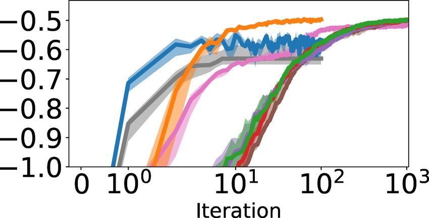
Marginalized Stochastic Natural Gradients for Black-Box Variational Inference
1.0 0 1 import torch
2 from pyro import poutine
3
−2
z1 z2
0.8 4 class MSNG:
5 ...
−4 6 def step(self, *args, **kwargs):
0.6
7 log_p = {}
μ1
−6 8 for group in self.variational_params:
0.4 9 log_p[group] = torch.zeros_like(self.variational_params[group])
x 0.2
−8
10
11 for s in range(self.num_samples):
12 # Sample z from the variational distribution
−10 13 guide_trace = poutine.trace(self.guide).get_trace(*args, **kwargs)
0.0 14
0.0 0.2 0.4 0.6 0.8 1.0 15 # Iterate over each variable (each group is a tensor,
μ2 16 # so variational_params[group][idx] is the actual individual variable)
17 for group in self.variational_params:
18 for idx in self._get_indices(group):
(a) Noisy-OR model (b) ELBO contour plot 19 # Remember actual sampled value of z_i
20 k0 = 1 * guide_trace.nodes[group]['value'][idx]
1.0 1.0 1.0 1.0 21
22 for k in range(self._get_K(group)):
23 # Condition z_i = k
0.8 0.8 0.8 0.8
24 guide_trace.nodes[group]['value'][idx] = torch.tensor(k)
25 model = poutine.replay(self.model, trace=guide_trace)
0.6 0.6 0.6 0.6 26 model_trace = poutine.trace(model).get_trace(*args, **kwargs)
27
μ1
μ1
28 # Compute log p(z_i = k, z_j, x)
0.4 0.4 0.4 0.4 29 model_log_p = self._compute_log_p(model_trace, group, idx)
30 log_p[group][idx][k] += model_log_p
31
0.2 0.2 0.2 0.2 32 # Change value of z_i back to k0
33 guide_trace.nodes[group]['value'][idx] = k0
0.0 0.0 0.0 0.0 34
0.0 0.2 0.4 0.6 0.8 1.0 0.0 0.2 0.4 0.6 0.8 1.0 35 for group in log_p:
μ2 μ2 36 # Compute log odds ratio
37 tau = log_p[group] / self.num_samples
38 tau_K = tau.index_select(-1, torch.tensor(self._get_K(group) - 1))
(c) REINFORCE (d) MSNG (ours) 39 tau -= tau_K
40
41 # Natural gradient ascent update
42 tau0 = self.variational_params[group]
43 self.variational_params[group] = (1 - lr) * tau0 + lr * tau
Figure 3. Pyro implementation of MSNG. This inference code
works for any discrete-variable model specified by valid Pyro
model and guide functions. See the supplement for further details.
algorithms) initially drop. But after only a few iterations,
(e) ELBO trace plot of MSNG, REINFORCE, and SCAVI MSNG robustly increases the ELBO again. Fig. 2(e) also
demonstrates that SCAVI (blue) lacks convergence guar-
Figure 2. (a): Graphical illustration of a toy noisy-OR model with
antees: even after achieving high ELBO values, “unlucky”
two latent variables z and one observation x = 1. (b): Contour
samples may regularly cause divergence.
plot of the model’s ELBO as a function of µ1 and µ2 . The yellow
star indicates the global maximum. Although the likelihood is 4.3. Generalization to Categorical Variables
symmetric with respect to z1 and z2 , the prior of z1 is higher, so
to explain x = 1, the optimal µ∗1 ≈ 0.99 and µ∗2 similar to its Our MSNG algorithm may be easily extended to general
prior. (c): The probability of ELBO increase after a REINFORCE categorical latent variables zi taking one of K discrete
gradient update of Eq. (8). (d): The probability of ELBO increase
after a MSNG update of Eq. (17). (e): ELBO trace plot of different h natural parameter of q(zi ) now becomes
states. The i a vec-
methods, with initial µ1 = 0.5, µ2 = 0.9. In (c-e), the sampling tor τi , log µµiK
i1
, . . . , log µµiK
ik
, . . . , log µµiK−1
iK
of length
budget M = 2, and the learning rate α = 0.5 in (c) and (d). K − 1. The MSNG update for each entry τik is
M (m)
new 1 X p(zi = k | z−i , x)
plot of the ELBO in Fig. 2(b), this is a simple optimization τik = α log (m)
+ (1 − α)τik .
problem with a global maximum indicated by the yellow star. M m=1 p(zi = K | z−i , x)
However, due to its high variance, the noisy REINFORCE A detailed derivation of this update is in the supplement,
gradient is more likely to decrease the ELBO than increase and Fig. 3 shows our general-purpose Pyro implementation.
it at every point in the blue region of Fig. 2(c). In contrast,
Our categorical MSNG update again has connections to
the variance of MSNG in Fig. 2(d) is much smaller, and the
exact CAVI updates (5), and is equivalent to the binary
promising red area around the global maximum makes it
MSNG update (17) when K = 2. Sato (2001) and Hoffman
more likely to “attract” variational parameters towards the
et al. (2013) discuss connections between natural gradients
global optimum. The ELBO trace plot in Fig. 2(e) verifies
and CAVI for continuous, conditionally conjugate models.
this, where MSNG (orange) converges much faster than RE-
INFORCE even with a well-tuned learning rate (red). We To enable black-box application of our MSNG variational
can see that many REINFORCE iterations with relatively inference method, our experiments focus on models where
high ELBO values actually decrease the ELBO, as predicted all latent variables are discrete. While the SNG estimator is
by the blue region around the optimum in Fig. 2(c). Notice easily generalized to continuous latent variables, methods
that we adversarially pick our initialization from the blue for (approximate) black-box marginalization of continuous
region in Fig. 2(d), so the ELBOs of MSNG (and other variables is left as a promising area for future research.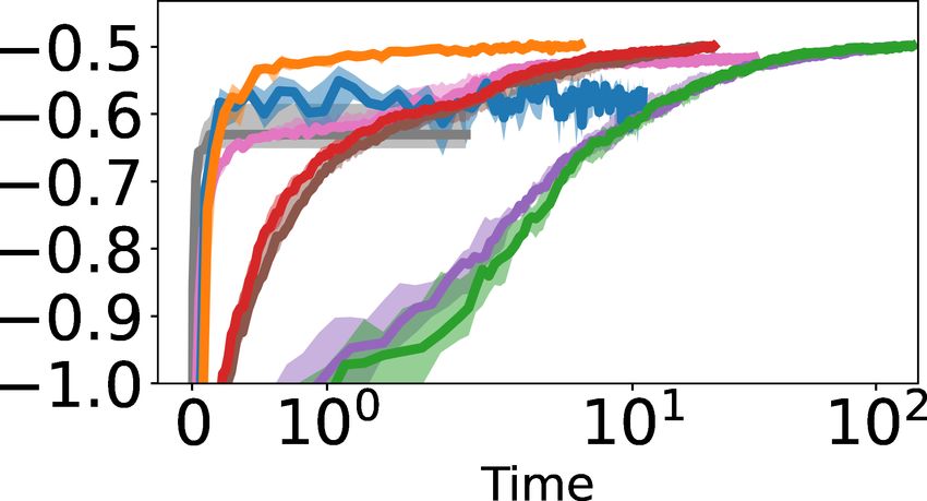
Marginalized Stochastic Natural Gradients for Black-Box Variational Inference

5. Experiments                                                   various relations between 14 countries between 1950 and
                                                                 1965 (Rummel, 1976). We choose the “conference” rela-
We compare our proposed MSNG algorithm with seven                tion, which consists of symmetric connections indicating if
other variational methods: the non-marginalized stochastic       two countries co-participate in any international conference.
natural gradients (SNG) of Sec. 4.1, standard score-function     The second dataset is about NeurIPS coauthorship (Glober-
gradients (REINFORCE), their improved versions with con-         son et al., 2007), where a link indicates two individuals
trol variates (SNG+CV and REINFORCE+CV), the heuris-             being coauthors of a paper in one of the first 17 NeurIPS
tic SCAVI method that approximates CAVI expectations in          conferences. Following Miller et al. (2009) and Palla et al.
Eq. (5) with Monte Carlo samples, the CONCRETE relax-            (2012), we model the 234 most connected authors. Model
ation based on Gumbel-Max sampling, and model-specific           parameters and Pyro specifications for these two models are
auxiliary-variable methods (AUX, for binary models only).        provided in the supplement, as well as an AUX algorithm
AUX methods are taken from prior work for noisy-OR (Ji           derived by us for the probit latent-feature model.
et al., 2019) and sigmoid belief networks (Gan et al., 2015),
and derived by us (extending Albert & Chib (1993)) for the       Annotation models for crowd-sourcing data. We test the
binary relational model’s probit likelihood.                     annotation model of Passonneau & Carpenter (2014) on two
                                                                 publicly available Amazon Mechanical Turk datasets (Snow
We integrate the black-box methods MSNG, SNG(+CV),               et al., 2008). The first dataset, on Recognizing Textual En-
and SCAVI into Pyro to make fair comparisons with the            tailment (RTE), has 800 questions and 164 annotators. For
already-supported REINFORCE(+CV) and CONCRETE.                   each question, the annotator is presented with two sentences
We use Pyro’s standard decaying average baseline2 to weight      to make a binary choice (K = 2) of whether the second
control variates, with the default decay rate of 0.9. MSNG       hypothesis sentence can be inferred from the first. The sec-
is also compatible with control variates, but it does not need   ond dataset, on Word Sense Disambiguation (WSD), has
a baseline CV because the latent variable associated with        177 questions and 34 annotators. The annotator is asked to
the score function in each dimension has been marginalized.      choose the most appropriate sense of a particular word in a
More experimental details are provided in the supplement.        sentence out of K = 3 possible options.

5.1. Models and Datasets                                         For the annotation model, we use the conjugacy of Dirichlet
                                                                 priors to analytically marginalize the unknown rater accu-
Noisy-OR topic graphs for text data. Following Ji et al.         racy distributions θjk . This leads to a “collapsed” variational
(2019), we infer topic activations in a noisy-OR topic model     bound that depends only on the posteriors q(zi ) for the
of documents from the “tiny” version of the 20 newsgroups        true category of each question (item). Collapsing induces
dataset collected by Sam Roweis. We use the same model           high-order dependencies that make classic CAVI updates
architecture, which has 44 latent topic nodes within two         intractable, but we show that our black-box MSNG updates
layers, and 100 observed token nodes. The edge weights w         are effective, while being simpler than previous collapsed
are learned on the training set through the full-model varia-    variational inference algorithms (Teh et al., 2007). See the
tional training method, with auxiliary bounds for noisy-OR       supplement for details about model hyperparameters.
likelihoods, described in the original paper. Their values are
then fixed as we compare the different variational inference     5.2. Comparison of Variational Inference Results
algorithms on 100 randomly subsampled test documents.
                                                                 Figs. 4 and 5 show the median ELBOs of different methods
Sigmoid belief networks for image data. On the binarized         across repeated runs, where the randomness is caused by
MNIST training dataset, we learn the edge weights w of a         Monte Carlo sampling (for stochastic methods) and the or-
three-layer fully-connected sigmoid belief network using the     der of parameter updates (for sequential methods). Like Gan
public data-augmented variational training code by Gan et al.    et al. (2015), the ELBOs are evaluated via Monte Carlo sam-
(2015). The top two layers each have 100 hidden nodes, and       pling. The algorithms compared with MSNG can be split
the observed bottom layer corresponds to the 28 × 28 pixels.     into four groups: unbiased gradient-based methods, the
Similar to noisy-OR topic model experiments, we fix the          heuristic SCAVI method, model-dependent AUX methods,
edge weight when testing the different inference algorithms      and the biased CONCRETE relaxation using continuous
on 100 images randomly selected from the MNIST test set.         variables. For clarity, we focus on one at a time below.
Fig. 1 shows Pyro specifications of our belief networks.
                                                                 MSNG converges much faster, and requires fewer sam-
Relational models for network data. We apply the two re-         ples, than competing unbiased BBVI methods. The con-
lational models described in Sec. 2.2 to two network datasets    vergence speed of a stochastic gradient method is influ-
used by Miller et al. (2009). The first dataset describes        enced by the learning rate and the sampling budget. We
   2
   https://pyro.ai/examples/svi part iii.html#                   find that MSNG is less sensitive to learning rates, and for
Decaying-Average-Baseline                                        all but the probit relational model, we choose a fixed rate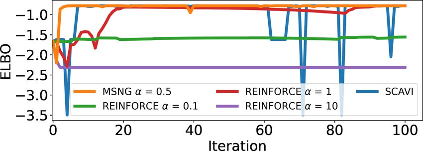
Marginalized Stochastic Natural Gradients for Black-Box Variational Inference

         MSNG          SNG         SNG + CV          REINFORCE          REINFORCE + CV            SCAVI        CONCRETE          AUX

    (a) Newsgroups (noisy-OR)             (b) MNIST (sigmoid)                (c) Countries (probit)           (d) NeurIPS (probit)

Figure 4. Improvement of ELBO (vertical axis) versus runtime (top row) and iteration (bottom row) on various models with binary
variables. Lines show the median, while shaded regions show the 25th and 75th percentiles, across 10 repeated runs.

         MSNG            SNG           SNG + CV            REINFORCE            REINFORCE + CV            SCAVI           CONCRETE

        (a) RTE (annotation)             (b) WSD (annotation)               (c) Countries (SBM)               (d) NeurIPS (SBM)

Figure 5. Improvement of ELBO (vertical axis) versus runtime on various models with categorical variables (performance versus iterations
is in the supplement). Lines show the median, while shaded regions show the 25th and 75th percentiles, across 10 repeated runs.

via grid search. SNG and REINFORCE (with or without                   and relational models of the larger NeurIPS data, neither
control variates) and CONCRETE show greater sensitiv-                 is able to effectively improve the ELBO with a budget of
ity, so as suggested by Ranganath et al. (2014) we use                M = 100 samples. Meanwhile, methods with control vari-
AdaGrad (Duchi et al., 2011) to adapt learning rates for              ate (SNG+CV and REINFORCE+CV) are able to make
SNG(+CV), REINFORCE(+CV), CONCRETE, and MSNG                          faster improvement to the ELBO, even with 10 times fewer
(probit only). For each method, we evaluate sample sizes              samples. Finally, MSNG always converges much faster than
of M ∈ {1, 10, 100}, and then report results for the variant          the other methods, even with just 1 sample per iteration.
that converges with lowest runtime. This leads to a sample
                                                                      Fig. 6 visualizes MNIST digit completion results using
size of M = 1 for MSNG; 100 for SNG and REINFORCE;
                                                                      the sigmoid belief network. REINFORCE and REIN-
and 10 (noisy-OR, sigmoid, Countries probit) or 100 (all
                                                                      FORCE+CV are clearly worse than MSNG, with even 10
else) for SNG+CV, REINFORCE+CV, and CONCRETE.
                                                                      or 100 times more samples. This performance is consistent
In Figs. 4 and 5, all methods share the same initialization,          with ELBO values of different methods in Fig 4(b).
and we run them until convergence or for a maximum of
                                                                      MSNG is more stable than SCAVI. With only one sample,
1,000 iterations. Across all eight model-dataset combina-
                                                                      the heuristic SCAVI method is also able to quickly improve
tions, a general trend of optimization speed is MSNG
                                                                      the ELBO in the first few iterations. But its ELBO values in
SNG+CV ≥ REINFORCE+CV  SNG ≥ REINFORCE.
                                                                      the final iterations are usually worse than MSNG, as shown
Note that plots use a logarithmic horizontal scale, and
                                                                      in Fig. 4 and 5, as well as tables in the supplement that report
MSNG often converges tens or even hundreds of times faster
                                                                      detailed results for each dataset. Unlike MSNG, SCAVI is
than other stochastic gradient methods, in terms of both
                                                                      not guaranteed to converge, as shown in the examples in
clock time and number of iterations. Marginalization and
                                                                      Fig. 7. We also observe that while SCAVI may increase
natural gradients are both important for peak performance.
                                                                      the ELBO faster in the first few iterations, it often runs
In simple problems such as the deep belief networks and               slower than MSNG when measured by the actual clock
relational models of the small countries data, SNG con-               time. This is because SCAVI has to sequentially update
verges faster than REINFORCE, showing the benefit of                  variational parameters, but MSNG is able to compute the
natural gradients. In harder cases like the annotation models         gradient updates for all variables in parallel.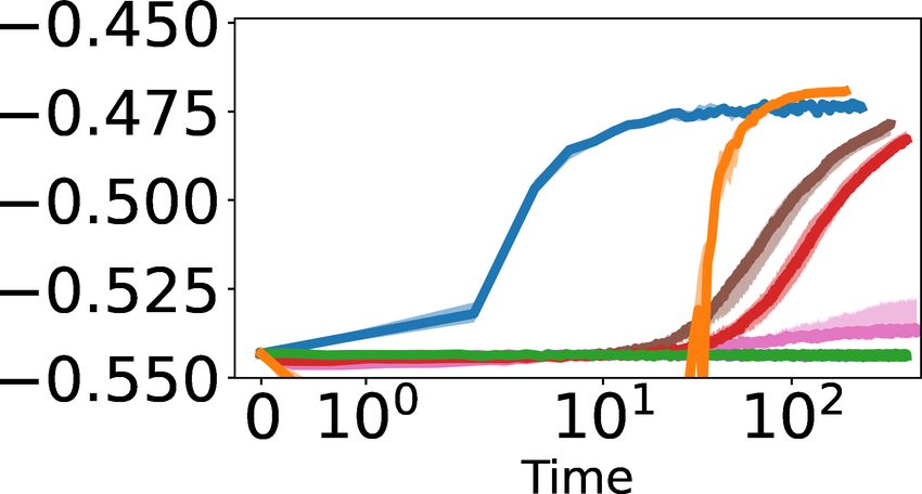
Marginalized Stochastic Natural Gradients for Black-Box Variational Inference
                                                                               MSNG        REINFORCE        REINFORCE + CV       SCAVI

                       (a) Original images

  (b) Digit completion: bottom parts of the images are missing
                                                                                   MNIST (sigmoid)                Countries (probit)
                                                                       Figure 7. ELBO trace plots of MSNG and other black-box varia-
                      (c) MSNG (1 sample)
                                                                       tional algorithms. Unlike the curves in Fig. 4 that are summarized
                                                                       across data and repeated runs, the ELBO here is just for one
                                                                       MNIST image (left) and a single run of the probit relation model
                 (d) REINFORCE (100 samples)                           (right), in order to reveal the non-convergence of SCAVI.

                                                                       models in Fig. 4(c-d) and Fig. 5(c-d) as an example. While
              (e) REINFORCE + CV (10 samples)                          the simple Countries data does not show a clear preference
                                                                       between the two models, the more complicated NeurIPS
                                                                       author data strongly favors the more powerful probit latent-
                      (f) SCAVI (1 sample)                             feature model over the stochastic block model.
                                                                       Biased CONCRETE updates achieve inferior ELBOs.
                                                                       CONCRETE updates more rapidly increase the ELBO than
                 (g) CONCRETE (10 samples)                             REINFORCE(+CV) in the first few iterations, but much
Figure 6. Digit completion results on binarized MNIST images.          of this advantage is lost when considering computation
We use upper halves of the images as observations to infer q(z),       time. Unlike all other methods we consider, CONCRETE
and fill in the lower halves by averaging 100 samples of x drawn       must (automatically) differentiate the model log-likelihood,
from q(z)p(x|z). The number of samples used during inference           which has time and memory overhead. CONCRETE is com-
(shown in the parentheses after each method) is matched to the         parable to MSNG and SCAVI for the annotation model; we
settings for Fig. 4(b). For all methods, the number of inference       hypothesize this is because the likelihood depends only on
iterations is 50, and the initial value for each latent node is 0.5.   histograms of many discrete variables, so continuous relax-
                                                                       ations are more accurate. But for other models, perhaps due
MSNG optimizes tighter bounds and is more robust to
                                                                       to its biased ELBO surrogate and sensitivity to the tempera-
initialization than AUX. In Fig. 4(b-d), model-dependent
                                                                       ture hyperparameter, CONCRETE results are inconsistent
AUX methods all converge to lower ELBO values than
                                                                       and often dramatically inferior to MSNG. Supplement Ta-
MSNG. This is likely because these methods all optimize
                                                                       bles D.1 and D.2 contain more detailed comparisons.
looser variational bounds than the original ELBO.
Another possible reason is that by introducing more param-             6. Discussion
eters into the objective, the optimization surface becomes             We have developed marginalized stochastic natural gradients
more complicated, and algorithms become more likely to                 (MSNG) for black-box variational inference in probabilistic
be trapped in local optima during sequential updates. Ran-             models with discrete latent variables. The MSNG method
domizing update order does not avoid this issue, as shown              has better theoretical guarantees, and converges much faster,
by the quantiles of AUX performance.                                   than REINFORCE. Unlike model-specific auxiliary meth-
                                                                       ods, MSNG directly optimizes a tighter likelihood bound,
In an additional experiment reported in the supplement,
                                                                       and is more robust to initialization in spite of being simpler
as suggested by Gan et al. (2015), we use the marginal
                                                                       to derive and implement. While our experiments focused
prior (as approximated by Monte Carlo) of each variable
                                                                       on models with only discrete variables, SNG updates are
in the sigmoid BN to initialize q(z). This engineering does
                                                                       easily extended to models that mix discrete and continuous
make AUX converge to better ELBOs than the uniform
                                                                       variables, and we are exploring applications to other model
initialization of Fig. 4(b), but MSNG is more robust and
                                                                       families. Our Pyro-integrated MSNG code provides a com-
converges to superior ELBOs for both initializations.
                                                                       pelling method for scalable black-box variational inference.
Finally, compared to hand-crafted auxiliary-variable algo-
rithms, the black-box property of MSNG allows for easy                 Acknowledgements
integration with PPL for convenient model selection. Users             This research supported in part by NSF CAREER Award No. IIS-
can easily and quickly fit different models on the same                1758028, NSF RI Award No. IIS-1816365, and a Facebook Proba-
dataset, and pick the best performing candidate with the               bility and Programming research award. We thank Prof. Alexander
highest ELBO values. Take the results of the two relational            Ihler for insightful suggestions in early stages of this work.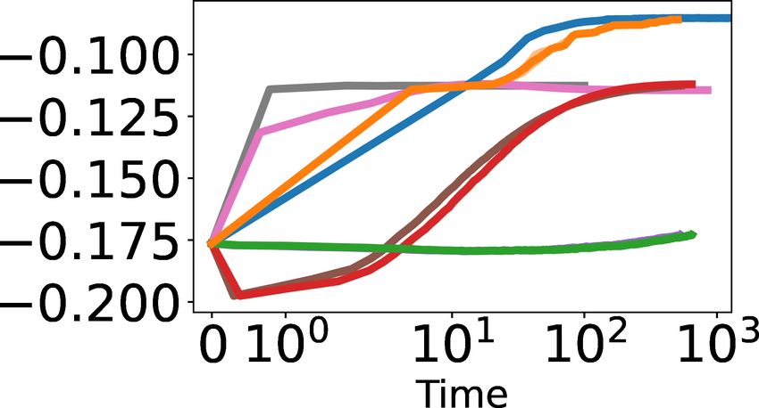
Marginalized Stochastic Natural Gradients for Black-Box Variational Inference

References                                                      Duchi, J., Hazan, E., and Singer, Y. Adaptive subgradient
                                                                  methods for online learning and stochastic optimization.
Albert, J. H. and Chib, S. Bayesian analysis of binary and
                                                                 Journal of machine learning research, 12(7), 2011.
  polychotomous response data. Journal of the American
  Statistical Association, 88(422):669–679, 1993.               Gan, Z., Henao, R., Carlson, D., and Carin, L. Learning
Amari, S.-I. Differential geometry of curved exponential          deep sigmoid belief networks with data augmentation. In
 families-curvatures and information loss. The Annals of         Artificial Intelligence and Statistics, 2015.
 Statistics, pp. 357–385, 1982.
                                                                Ghadimi, S. and Lan, G. Optimal stochastic approxima-
Amari, S.-I. Natural gradient works efficiently in learning.      tion algorithms for strongly convex stochastic composite
 Neural computation, 10(2):251–276, 1998.                         optimization I: A generic algorithmic framework. SIAM
                                                                 Journal on Optimization, 22(4):1469–1492, 2012.
Arjevani, Y., Carmon, Y., Duchi, J. C., Foster, D. J.,
  Srebro, N., and Woodworth, B. Lower bounds for                Ghadimi, S. and Lan, G. Stochastic first-and zeroth-order
  non-convex stochastic optimization. arXiv preprint              methods for nonconvex stochastic programming. SIAM
  arXiv:1912.02365, 2019.                                        Journal on Optimization, 23(4):2341–2368, 2013.

Bingham, E., Chen, J. P., Jankowiak, M., Obermeyer, F.,         Globerson, A., Chechik, G., Pereira, F., and Tishby, N.
  Pradhan, N., Karaletsos, T., Singh, R., Szerlip, P., Hors-      Euclidean embedding of co-occurrence data. Journal of
  fall, P., and Goodman, N. D. Pyro: Deep universal prob-         Machine Learning Research, 8:2265–2295, 2007.
  abilistic programming. Journal of Machine Learning
  Research, 20(1):973–978, 2019.                                Goodman, N. D. and Stuhlmüller, A. The Design and Im-
                                                                  plementation of Probabilistic Programming Languages.
Blei, D. M., Ng, A. Y., and Jordan, M. I. Latent Dirichlet        http://dippl.org, 2014.
  allocation. Journal of Machine Learning Research, 3:
  993–1022, 2003.                                               Gopalan, P., Hao, W., Blei, D. M., and Storey, J. D. Scaling
                                                                  probabilistic models of genetic variation to millions of
Blei, D. M., Kucukelbir, A., and McAuliffe, J. D. Varia-          humans. Nature genetics, 48(12):1587, 2016.
  tional inference: A review for statisticians. Journal of
  the American Statistical Association, 112(518):859–877,       Gopalan, P. K. and Blei, D. M. Efficient discovery of over-
  2017.                                                           lapping communities in massive networks. Proceedings
                                                                  of the National Academy of Sciences, 110(36):14534–
Bottou, L. Online learning and stochastic approximations.        14539, 2013.
  On-line learning in neural networks, 17(9):142, 1998.
                                                                Grathwohl, W., Choi, D., Wu, Y., Roeder, G., and Duve-
Carpenter, B., Gelman, A., Hoffman, M. D., Lee, D.,
                                                                  naud, D. Backpropagation through the void: Optimizing
  Goodrich, B., Betancourt, M., Brubaker, M. A., Guo,
                                                                  control variates for black-box gradient estimation. In
  J., Li, P., and Riddell, A. Stan: A probabilistic program-
                                                                  International Conference on Learning Representations,
  ming language. Journal of Statistical Software, 76(1):
                                                                  2018.
  1–32, 2017.

Casella, G. and Robert, C. P. Rao-Blackwellisation of sam-      Greensmith, E., Bartlett, P. L., and Baxter, J. Variance
  pling schemes. Biometrika, 83(1):81–94, 1996.                   reduction techniques for gradient estimates in reinforce-
                                                                  ment learning. Journal of Machine Learning Research, 5:
Cusumano-Towner, M. F., Saad, F. A., Lew, A. K., and              1471–1530, 2004.
  Mansinghka, V. K. Gen: A general-purpose probabilis-
  tic programming system with programmable inference.           Hoffman, M. D., Blei, D. M., Wang, C., and Paisley, J.
  In Conference on Programming Language Design and                Stochastic variational inference. Journal of Machine
  Implementation, 2019.                                          Learning Research, 14(1):1303–1347, 2013.

Dong, Z., Mnih, A., and Tucker, G. Disarm: An antithetic        Holland, P. W., Laskey, K. B., and Leinhardt, S. Stochastic
  gradient estimator for binary latent variables. In Advances     blockmodels: First steps. Social networks, 5(2):109–137,
  in Neural Information Processing Systems, 2020.                1983.

Drori, Y. and Shamir, O. The complexity of finding station-     Horvitz, E. J., Breese, J. S., and Henrion, M. Decision theory
  ary points with stochastic gradient descent. In Interna-        in expert systems and artificial intelligence. International
  tional Conference on Machine Learning, 2020.                    Journal of Approximate Reasoning, 2(3):247–302, 1988.
Marginalized Stochastic Natural Gradients for Black-Box Variational Inference
Jaakkola, T. S. and Jordan, M. I. Variational probabilistic Paisley, J. W., Blei, D. M., and Jordan, M. I. Variational
inference and the QMR-DT network. Journal of Artificial Bayesian inference with stochastic search. In Interna-
Intelligence Research, 10:291–322, 1999. tional Conference on Machine Learning, 2012.
Jang, E., Gu, S., and Poole, B. Categorical reparameteriza- Palla, K., Knowles, D. A., and Ghahramani, Z. An infinite
tion with gumbel-softmax. In International Conference latent attribute model for network data. In International
on Learning Representations, 2017. Conference on Machine Learning, 2012.
Ji, G., Cheng, D., Ning, H., Yuan, C., Zhou, H., Xiong,
Papandreou, G. and Yuille, A. L. Perturb-and-map random
L., and Sudderth, E. B. Variational training for large-
fields: Using discrete optimization to learn and sample
scale noisy-OR Bayesian networks. In Conference on
from energy models. In International Conference on
Uncertainty in Artificial Intelligence, 2019.
Computer Vision, 2011.
Jordan, M. I., Ghahramani, Z., Jaakkola, T. S., and Saul,
L. K. An introduction to variational methods for graphical Passonneau, R. J. and Carpenter, B. The benefits of a model
models. Machine Learning, 37(2):183–233, 1999. of annotation. Transactions of the Association for Com-
putational Linguistics, 2:311–326, 2014.
Kakade, S. M. A natural policy gradient. Advances in
Neural Information Processing Systems, 2001. Polson, N. G., Scott, J. G., and Windle, J. Bayesian in-
ference for logistic models using Pólya–Gamma latent
Kingma, D. P. and Welling, M. Auto-encoding variational
variables. Journal of the American statistical Association,
Bayes. In International Conference on Learning Repre-
108(504):1339–1349, 2013.
sentations, 2014.
Kucukelbir, A., Tran, D., Ranganath, R., Gelman, A., and Rakhlin, A., Shamir, O., and Sridharan, K. Making gradient
Blei, D. M. Automatic differentiation variational infer- descent optimal for strongly convex stochastic optimiza-
ence. Journal of Machine Learning Research, 18(1): tion. In International Conference on Machine Learning,
430–474, 2017. 2012.
Kullback, S. and Leibler, R. A. On information and suf- Ranganath, R., Gerrish, S., and Blei, D. M. Black box vari-
ficiency. The annals of mathematical statistics, 22(1): ational inference. In Artificial Intelligence and Statistics,
79–86, 1951. 2014.
Liu, J., Ren, X., Shang, J., Cassidy, T., Voss, C. R., and Han, Rezende, D. J., Mohamed, S., and Wierstra, D. Stochastic
J. Representing documents via latent keyphrase inference. backpropagation and approximate inference in deep gen-
In International Conference on World Wide Web, 2016. erative models. In International Conference on Machine
Liu, R., Regier, J., Tripuraneni, N., Jordan, M. I., and Learning, 2014.
McAuliffe, J. Rao-Blackwellized stochastic gradients
Ritchie, D., Horsfall, P., and Goodman, N. D. Deep amor-
for discrete distributions. In International Conference on
tized inference for probabilistic programs. arXiv preprint
Machine Learning, 2019.
arXiv:1610.05735, 2016.
Maddison, C. J., Mnih, A., and Teh, Y. W. The concrete
distribution: A continuous relaxation of discrete random Rummel, R. J. Attributes of nations and behavior of na-
variables. In International Conference on Learning Rep- tion dyads, 1950-1965. Inter-university Consortium for
resentations, 2017. Political Research, 1976.
Miller, K., Jordan, M. I., and Griffiths, T. L. Nonparametric Sato, M.-A. Online model selection based on the variational
latent feature models for link prediction. In Advances in Bayes. Neural Computation, 13(7):1649–1681, 2001.
Neural Information Processing Systems, 2009.
Schulman, J., Levine, S., Abbeel, P., Jordan, M., and Moritz,
Murphy, K. P. Machine Learning: A Probabilistic Perspec- P. Trust region policy optimization. In International
tive. MIT press, 2012. Conference on Machine Learning, 2015.
Neal, R. M. Connectionist learning of belief networks.
Artificial Intelligence, 56(1):71–113, 1992. Shwe, M. A., Middleton, B., Heckerman, D. E., Hen-
rion, M., Horvitz, E. J., Lehmann, H. P., and Cooper,
Nemirovsky, A. S. and Yudin, D. B. Problem complexity and G. F. Probabilistic diagnosis using a reformulation of
method efficiency in optimization. Society for Industrial the INTERNIST-1/QMR knowledge base. Methods of
and Applied Mathematics, 1983. Information in Medicine, 30(4):241–255, 1991.Marginalized Stochastic Natural Gradients for Black-Box Variational Inference
Singer, Y. and Vondrák, J. Information-theoretic lower Ye, L., Beskos, A., De Iorio, M., and Hao, J. Monte Carlo
bounds for convex optimization with erroneous oracles. co-ordinate ascent variational inference. Statistics and
In Advances in Neural Information Processing Systems, Computing, pp. 1–19, 2020.
2015.
Yellott Jr, J. I. The relationship between Luce’s choice ax-
Šingliar, T. and Hauskrecht, M. Noisy-OR component analy- iom, Thurstone’s theory of comparative judgment, and the
sis and its application to link analysis. Journal of Machine double exponential distribution. Journal of Mathematical
Learning Research, 7:2189–2213, 2006. Psychology, 15(2):109–144, 1977.
Snow, R., O’connor, B., Jurafsky, D., and Ng, A. Y. Cheap Yin, M. and Zhou, M. ARM: Augment-REINFORCE-
and fast–but is it good? evaluating non-expert annota- merge gradient for stochastic binary networks. In Inter-
tions for natural language tasks. In Empirical Methods in national Conference on Learning Representations, 2019.
Natural Language Processing, 2008.
Zhang, C., Bütepage, J., Kjellström, H., and Mandt, S. Ad-
Teh, Y. W., Newman, D., and Welling, M. A collapsed vari- vances in variational inference. Pattern Analysis and
ational Bayesian inference algorithm for latent Dirichlet Machine Intelligence, 41(8):2008–2026, 2018.
allocation. In Advances in Neural Information Processing
Systems, 2007.
Thomas, V., Pedregosa, F., Merriënboer, B., Manzagol, P.-
A., Bengio, Y., and Le Roux, N. On the interplay between
noise and curvature and its effect on optimization and
generalization. In Artificial Intelligence and Statistics,
2020.
Titsias, M. K. and Lázaro-Gredilla, M. Local expectation
gradients for black box variational inference. In Advances
in Neural Information Processing Systems, 2015.
Tran, D., Kucukelbir, A., Dieng, A. B., Rudolph, M., Liang,
D., and Blei, D. M. Edward: A library for probabilis-
tic modeling, inference, and criticism. arXiv preprint
arXiv:1610.09787, 2016.
Tran, D., Hoffman, M. W., Moore, D., Suter, C., Vasudevan,
S., and Radul, A. Simple, distributed, and accelerated
probabilistic programming. In Advances in Neural Infor-
mation Processing Systems, 2018.
Tucker, G., Mnih, A., Maddison, C. J., Lawson, J., and Sohl-
Dickstein, J. Rebar: Low-variance, unbiased gradient
estimates for discrete latent variable models. In Advances
in Neural Information Processing Systems, 2017.
Wainwright, M. J. and Jordan, M. I. Graphical models, ex-
ponential families, and variational inference. Foundations
and Trends in Machine Learning, 1:1–305, 2008.
Williams, R. J. Simple statistical gradient-following algo-
rithms for connectionist reinforcement learning. Machine
Learning, 8(3-4):229–256, 1992.
Wingate, D. and Weber, T. Automated variational in-
ference in probabilistic programming. arXiv preprint
arXiv:1301.1299, 2013.
Winn, J. and Bishop, C. M. Variational message passing.
Journal of Machine Learning Research, 6:661–694, 2005.You can also read