Impacts of Tide Gate Modulation on Ammonia Transport in a Semi-closed Estuary during the Dry Season-A Case Study at the Lianjiang River in South China
←
→
Page content transcription
If your browser does not render page correctly, please read the page content below
water
Article
Impacts of Tide Gate Modulation on Ammonia
Transport in a Semi-closed Estuary during the Dry
Season—A Case Study at the Lianjiang River
in South China
Changjin Zhao 1 , Hanjie Yang 1 , Zhongya Fan 1, * , Lei Zhu 2 , Wencai Wang 1 and Fantang Zeng 1
 1   National Key Laboratory of Water Environmental Simulation and Pollution Control, Guangdong Key
     Laboratory of Water and Air Pollution Control, South China Institute of Environmental Sciences, Ministry
     of Ecology and Environment, No. 18 Ruihe Road, Guangzhou 510530, China; zhaochangjin@scies.org (C.Z.);
     yanghanjie@scies.org (H.Y.); wangwencai@scies.org (W.W.); zengfantang@scies.org (F.Z.)
 2   School of Marine Science, Sun Yat-sen University, 135 Xingangxi Rd., Guangzhou 510275, China;
     zhulei28@mail.sysu.edu.cn
 *   Correspondence: fanzhongya@scies.org; Tel.: +020-85544702

 Received: 5 June 2020; Accepted: 29 June 2020; Published: 9 July 2020

 Abstract: Recovery of tide-receiving is considered to improve the water quality in the Lianjiang River,
 a severely polluted and tide-influenced river connected to the South China Sea. A tide-receiving
 scenario, i.e., keeping the tide gate open, is compared with the other scenario representing
 the non-tide-receiving condition, i.e., blocking the tide flow during the flood phase, by numerical
 simulations based on the EFDC (Environmental Fluid Dynamics Code) model. The impacts of
 tide receiving were evaluated by the variation in the concentration of ammonia and its exporting
 fluxes, mainly in the downstream part of the river. With more water mass coming into the river,
 in the tide-receiving scenario, the averaged concentration of ammonia reduced by 20–40%, with
 the most significant decrease of 0.64 g m−3 . However, the exporting flux of ammonia has decreased
 in the tide-receiving scenario, as the consequence of the back–forth oscillation of tidal current.
 In the tide-receiving scenario, the time series of ammonia concentration approximately followed
 the tidal oscillation, with increased concentration during the ebb tide and reduction in the flood
 tide. In the non-tide-receiving scenario, the ammonia concentration decreases when the tide gate is
 open which results in further intrusion of seawater. This was followed by an increase in ammonia
 concentration again after the currents shift seaward and water mass with higher concentration
 from the upstream part is transported downstream. Given the identical ammonia input and river
 runoff, the ammonia concentration stays lower in the tide-receiving scenario, except for short periods
 after the tide gate opening and neap tides in the downstream part which lasts for around half
 a day. This study highlights the importance of hydrodynamic condition, specifically tidal oscillation,
 in the semi-diurnal and fortnight cycles, for the transportation of waterborne materials. Furthermore,
 the operation of the tide gate was additionally discussed based on potential varied practical conditions
 and evaluation criteria.

 Keywords: tide gate; ammonia transport; tide-influenced river; estuary

1. Introduction
    The highly urbanized estuary and coastal areas, due to its high industrialization, with dense
popularity and variability of near-coastal systems, are susceptible to multiple pressures induced by
anthropological influence [1–3]. In the last century, the increased demand for agricultural irrigation,

Water 2020, 12, 1945; doi:10.3390/w12071945                                       www.mdpi.com/journal/water
Water 2020, 12, 1945                                                                                  2 of 17

limited availability of freshwater, and the requirement to protect lands from inundation and salty
water intrusion have initiated the building of water infrastructures, such as tide gates, worldwide [4].
Tide gates are generally doors or flaps mounted on the downstream ends of rivers near the sea,
which allow upstream waters to drain while preventing inflows from the sea due to tidal surges or
flood events [5,6]. However, tide gate could disrupt the natural ecosystem by reducing the water
connectivity between the river and sea, which potentially would result in undesirable physical,
chemical, and biological side effects, such as low dissolved oxygen, high nutrients concentration and
intensified algae bloom [7,8], blocked or delayed fish passage [9], invasion of upland plant, and so on.
Additionally, in some areas where local industries have experienced rapid development, the degraded
water connectivity could further deteriorate undesirable water quality [10]. In recent decades, easing
the conflicts between economic development and environmental capacity is not only the urgent desire
of public members to improve life quality, but also an important guarantee for cities and promoting
sustainable economic and social development [11]. Taking account of the pros and cons of coastal
infrastructure, how to utilize or restore the previously constructed tide gate to adapt to the new
requirements of economic and environmentally friendly development, has drawn increasing attention
and been under fierce debate [12].
      To improve the flushing of tide-gate-controlled rivers has long been recognized as an important
part of solving the problem of undesired water quality in poorly water-connected rivers [13,14]. This is
precisely the major concern of this study, the replaned operation of the tide gate at the Haimen Bay
(HMB). The tide gate was firstly built in 1970 at the Lianjiang River in the southern part of China.
It blocked the salty water inflow from the sea and overflow is only allowed when the water head
in the upper stream is too high for the stock. Even though the local development has benefited
from the tide gate’s operation for the past several decades, the operation of the tide gate has resulted
in a longer residual time of pollutants discharged by industries in the river upstream basin, which
has caused critical levels of contamination [15]. To mitigate the severely polluted condition and help
the ecological recovery, the reconstructed two-way tide gate at HMB to recover the tide receiving is
expected to speed up the dispersion and advection of pollutants in the upstream. Besides the expected
positive consequence, some negative impacts are also foreseeable, for example, increasing salty
water intrusion and intensifying flushing of sediments [16]. Identification of the best practice to
improve water quality as well as avoid saltwater intrusion and mitigate possible undesirable influence
in the downstream part, however, is still a matter of further investigation and quantitative analysis.
      To what extent the recovered tide-receiving could influence the pollutants’ concentration and
export flux merits quantization and concrete plan for environmental initiatives. Particularly for
tide-influenced rivers and estuaries, tidal characteristics play an important role in the transport and
concentration of sediments and waterborne materials [17,18]. As a typical tide-influenced river,
the hydrodynamic transport in the Lianjiang River consists of processes characterized by different
time scales. On the time scale of hours, floods and ebbs of semi-diurnal tidal cycles induce back–forth
flow which results in periodical intrusion of seawater and flushing out of river water mass. The daily
tidal cycle is further superposed by a fortnightly change of tide with a period of around half a month.
Furthermore, other physical factors, such as precipitation rate, wind, river discharge varying in seasonal
range in the Lianjiang Basin, will further complicate the situation. The tide flow, with interacting
river runoff, determines the intrusion of salinity, resuspension of particulate matter, and dilution
of pollutants.
      In this study, based on the validated EFDC setup designed for the Lianjiang River, a scenario with
tide-receiving (tide gate is kept open for the whole simulation period) was compared to a scenario
without tide-receiving (i.e., the tide gate is open during the ebb tide, as historically planned). Simulation
time was arranged in the dry season when the river is normally at a greater risk of pollution. Ammonia
nitrogen was selected to represent the transport and distribution of pollutants. Besides the quantitative
assessment of the improvements in the water quality, mechanisms accounting for the spatial and
temporal variability of nitrogen’s distribution is further investigated. The specific questions of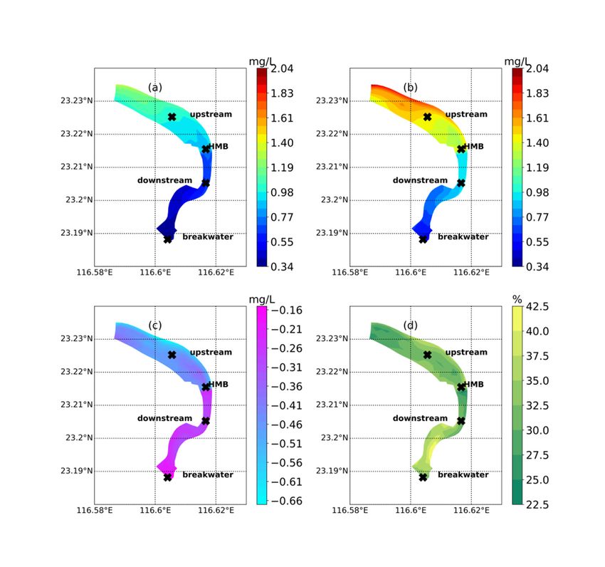
Water 2020, 12, 1945                                                                                 3 of 17

this study plan to resolve are: (1) quantifying the improvements in water quality, spatially and
temporally, resulted from the tide receiving. (2) Pointing out the difference in time series of currents
and nitrogen, modulated by the operation of the tide gate. (3) Quantifying the difference driven by
the spring–neap cycle.
     In the following sections, we first introduce the local natural and social characteristics of
the Lianjiang River. Second, we provided the setting of the numerical model, the design of scenarios,
and analyzing the routine of results. Third, in the result part, after the validation of the model setup,
the variations of water quality in different scenarios were laid out and discussed. In the discussion
part, we further explored the mechanisms responsible for the dispersion and dilution processes
in the downstream part, in the context of hydrodynamic characteristics. The planning of tide
receiving and its consequences were additionally discussed based on varied practical conditions and
environmental criteria.

2. Materials and Methods

2.1. Study Site
      Lianjiang River is one of the major rivers which flow into the South China Sea on the coast of
eastern Guangdong province. The catchment area of the Lianjiang River is 1353 km2 , with the center
of the basin located at 116.33◦ E, 23.26◦ N. The total population within this area is 4.67 million.
The mainstream, with a length of 71 km, connects to the sea at its southern end the breakwater (Figure 1)
and extends inland at the Puning city at 166.15◦ E, 23.36◦ N. The annual average runoff of the basin
is 1.353 billion m3 and the average annual rainfall is 1618 mm. The runoff and rainfall are unevenly
distributed throughout the year, with less amount in winter and spring and more in summer and
autumn. The seasonal variation in rainfall is related to the typical Southeast Asian monsoon climate.
The southeast wind prevails in summer and northwest wind dominates in winter. The average wind
speed for multiple years is 2.1 m s−1 , with a maximum wind speed of about 26 m s−1 . For the HMB,
in addition to the fluvial influence, the impact of the ocean could further complicate the physical or even
biological conditions. Currents flow along the coast of the Guangdong province, in the south-western
to north-western direction, may add the influence of river runoff of the Pearl River (Figure 1) and
nutrients input along the coast [19–21]. Driven by the south-western monsoon in summer, the Ekman
transport tends to bring the surface water away from the coast. Therefore, the upwelling system
adds a water body with high nutrients, high salinity, and low dissolved oxygen and temperature to
the coastal water in the concerned area [22–24].
      The tide gate at the HMB is a large-scale water conservancy project that was initially designed
to prevent saltwater intrusion and improve the storage of freshwater. The tide gate is located near
Haimen Town at the estuary of Lianjiang River, which is 2 km away from the river mouth (Figure 1).
Since the 1970s, the operation of this tide gate has basically reduced the salty water intrusion caused by
typhoons on more than 300,000 acres of farmland. It has effectively improved the irrigation of 187,000
acres of farmland on both sides of the Lianjiang River and guaranteed the water supply of living and
industry use for more than 1,000,000 people.
      Even though the local development has benefited from the tide gate’s operation, the wetland
ecosystems of the Lianjiang Estuary have been significantly changed. Since the 1990s, due to
the population growth, the development of the textile printing and dyeing industry along the river,
the pollutant loading has exceeded the ecological capacity [25]. The nutrients’ concentration has long
been below the inferior class V according to the Chinese Environmental Quality Standard for Surface
Water (GB3838-2002; chemical oxygen demand (COD) > 40 mg L−1 , NH4 > 2 mg L−1 , total phosphate
(TP) > 0.4 mg L−1 , dissolved oxygen (DO) < 2 mg L−1 ). In the lower reaches of the Lianjiang River,
the water quality has not met the demand for production and living water in fisheries for a long time.
The Lianjiang Estuary wetland ecosystem has almost lost its ecological service functions.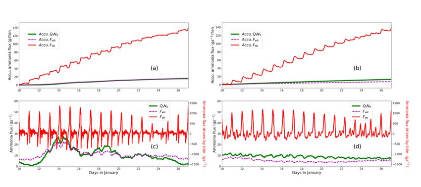
Water 2020, 12, 1945                                                                                            4 of 17
   Water 2020, 12, x FOR PEER REVIEW                                                                               4 of 20

     Figure 1. Bathymetry of the simulation domain. Cross-sections used for time series analysis are marked
     out by black diamonds and for flux calculations by black crosses. Open boundaries of upper and lower
        Figure
     limits      1. Bathymetry
            are depicted          of dot
                         by a black  the and
                                          simulation
                                              a magentadomain.    Cross‐sections
                                                          line, respectively.     used shows
                                                                              The inset for time
                                                                                              the series analysis
                                                                                                  northern part of are
        marked    out by black  diamonds    and  for flux calculations  by black crosses.
     the South China Sea and the Lianjiang Basin which is enclosed by the red rectangle.  Open  boundaries   of upper
        and lower limits are depicted by a black dot and a magenta line, respectively. The inset shows the
     Thenorthern   part of the
          reconstruction     ofSouth  China
                                the tide gateSea  and the
                                                began       Lianjiang of
                                                        in October    Basin
                                                                         2018 which
                                                                               and is enclosedtoby
                                                                                    planned      bethe red rectangle.
                                                                                                    complete    in May
of 2021. Before the restoration, the tide gate was planned to open during the ebb–tidal phase for
        The
draining.    tidethe
          After   gateebbattide,
                             the the
                                 HMB     is a large‐scale
                                     aquifer    area in the water
                                                            upperconservancy      project
                                                                   stream is refilled  withthat  was The
                                                                                             runoff.  initially  designed
                                                                                                            draining  is
   to prevent
more  frequentsaltwater      intrusion
                in flood season     thanandthatimprove    theseason.
                                                 in drought   storageTheof freshwater.  The tide
                                                                            specific operation   of gate  is located
                                                                                                    the tide  gate hasnear
been determined by many anthropogenic factors, such as reservoir operation in the upstream, water 1).
   Haimen   Town    at  the estuary   of  Lianjiang    River, which  is 2 km  away   from   the river mouth    (Figure
   Sincelevel
surface  the 1970s,   the operation
              in the upstream,     andof    this tidefor
                                        demands       gate has basically
                                                         sewage  draining. reduced   therestoration,
                                                                              After the  salty watertheintrusion   caused
                                                                                                           tide gate  is
   by typhoons
proposed          on more
          to be kept           than
                        open for  the300,000
                                      whole dry acres  of farmland.
                                                     season when theItpollution
                                                                         has effectively   improved
                                                                                  risk is severe        the irrigation
                                                                                                  and more     dilution of
and187,000  acresare
     dispersion    of demanded.
                       farmland on both sides of the Lianjiang River and guaranteed the water supply of
   living and industry use for more than 1,000,000 people.
2.2. Numerical  Model the local development has benefited from the tide gate’s operation, the wetland
        Even though
   ecosystems of the Lianjiang Estuary have been significantly changed. Since the 1990s, due to the
     The EFDC model, originally developed at the Virginia Institute of Marine Science and later
   population growth, the development of the textile printing and dyeing industry along the river, the
sponsored by the US Environmental Protection Agency (USEPA), is a modeling package for simulating
   pollutant loading has exceeded the ecological capacity [25]. The nutrients’ concentration has long
2D or 3D hydrodynamic fields coupled with several biogeochemical processes. Multiple modules
   been below the inferior class V according to the Chinese Environmental Quality Standard for Surface
are responsible to resolve varied components in the water environment, such as sediments and
   Water (GB3838‐2002; chemical oxygen demand (COD) > 40 mg L−1, NH4 > 2 mg L−1, total phosphate
benthic substances, toxic contaminants, microalgae growth, and nutrient cycling. It has been applied
   (TP) > 0.4 mg L−1, dissolved oxygen (DO) < 2 mg L−1). In the lower reaches of the Lianjiang River, the
worldwide in various surface water systems, such as rivers [26], lakes [27], estuaries [28], wetlands,
   water quality has not met the demand for production and living water in fisheries for a long time.
and coastal regions [29]. The model solves the vertically hydrostatic, free-surface, turbulent averaged
   The Lianjiang Estuary wetland ecosystem has almost lost its ecological service functions.
equations of motion for a variable-density fluid, using second-order accurate spatial finite-difference
        The reconstruction of the tide gate began in October of 2018 and planned to be complete in May
on a staggered C grid. Vertically, the sigma vertical coordinates are applied. The Mellor–Yamada level
   of 2021. Before the restoration, the tide gate was planned to open during the ebb–tidal phase for
2.5 turbulence closure scheme [30] is used to calculate turbulence parameters. Details of governing
   draining. After the ebb tide, the aquifer area in the upper stream is refilled with runoff. The draining
equations and numerical schemes for the EFDC hydrodynamic model are given by [31]. The code
   is more frequent in flood season than that in drought season. The specific operation of the tide gate
version 7.1 of EFDC was applied in this study. To simulate structural obstacles which blocks flow
   has been determined by many anthropogenic factors, such as reservoir operation in the upstream,
   water surface level in the upstream, and demands for sewage draining. After the restoration, the tide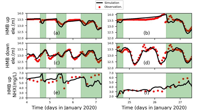
Water 2020, 12, 1945                                                                                  5 of 17

across specified cell faces, in the EFDC model, the “mask.inp” function is designed to insert thin
barriers which have widths much less than cell size or one grid spacing. Particularly, in this study,
to implement the tide gate operation which is varying with time, the “mask.inp” was modified to play
the “blocking” role in appointed time steps.

2.3. Model Setting
      The simulation domain covers nearly a 30 km segment of the downstream part of the Lianjiang
River (Figure 1). To the north, the open boundary of the upstream reaches a Lianjiang sluice
in the mainstream, which is marked out in black dots in Figure 1. To the south, it includes the adjacent
coastal area where the bay connects to the open sea. The magenta line represents the open boundary
of the seaside (Figure 1). Along the river, several major tributaries have been resolved (Figure 1),
with additional runoff and ammonia loading. Locations of the tide gate at the HMB and 2 other
representative cross-sections, namely, the upstream cross-section relative to the HMB (UH) and
the downstream cross-section relative to the HMB (DH), are marked out in black diamonds in Figure 1.
Depicted by black crosses, the cross-sections of HMB and breakwater are used for flux calculation for
the downstream portion (Figure 1). The model was formulated on orthogonal curve coordinate grids,
with a spatial resolution ranging from 100 to 300 m. In total, it has 6264 simulation cells in the horizontal
direction, with 5 layers in the vertical direction in the sigma coordinates. The model time step was 2.5 s
and the output time step is 20 min, which allows for a robust representation of processes of physics and
biogeochemistry. In the water quality module, dissolved oxygen (DO), total phosphate (TP), ammonia
nitrogen (NH4 ), and chemical oxygen demand (COD) were simulated. The benthic flux of ammonia is
14.4 mg m−2 day−1 [32,33] Nitrification and denitrification rates are set to be 0.1 day−1 , 0.09 day−1 [34].
The manning coefficient is set as 0.02.
      In the setup, necessary boundary and initial conditions were prescribed, including bathymetric
information, meteorological conditions, loading of ammonia, and operation of the tide gate.
The bathymetry in the Lianjiang River was measured in 2014 by the Shantou Hydrological Branch
of Guangdong Hydrographic Bureau. The topographic of the study area is interpolated results
of the nautical charts. The meteorological condition was provided by the Chinese Meteorological
Science Data Sharing Service Network (http://data.cma.cn/). The data were originally measured
at the meteorological station (116.58◦ E, 23.27◦ N) near the Lianjiang River. Among the measured
meteorological data, wind, temperature, relative humidity, and water vapor pressure were implemented
in the setup. The boundary of the study area was driven by the water elevation obtained from the Global
Tide Assimilation Data (OTIS) [35], which was developed by Oregon State University in the United
States. Sea surface elevation was prescribed at the open boundary of the with a time step of 1 h, which
was sufficient to represent daily and half-month cycles. The eight most important tidal constituents
(M2 , S2 , N2 , K2 , K1 , O1 , P1 , Q1 ) are considered in the boundary forcing. Principal lunar (M2 ) and
principal solar (S2 ) tides are responsible for most of the sea level variations in the semi-diurnal
period, superposed by the fortnightly modulation due to the beating of the M2 , S2 . Relieving of
diurnal inequality of tides during the neap phase has also been resolved properly. The water quality
module and the field of salinity were initiated by the on-site water quality monitoring data of the area.
Pollutants from tributaries were implemented as point sources entering the mainstream. By taking
account of the distribution of sewage treatment plants and administrative divisions of sewage outlets,
corresponding fluxes of pollutants were generalized into constant values for each tributary to represent
spatial patterns of pollutants loading, particularly for the dry season. The full simulation period
encompasses 35 days, which was initialized on 1 January, 2020 and ended on 5 February, 2020.
The selected period is representative of the dry season of the Lianjiang River, when the polluted
condition is generally more serious and water quality risk is higher than that in the wet season. For the
validation, the simulation is forced with observed river runoff and ammonia concentration in January
of 2020. The river runoff during that period fluctuated between 5–13 m3 s−1 . Ammonia concentration
was in the range of 4–9 mg L−1 . For the scenario analysis, in order to focus on the difference in ammonia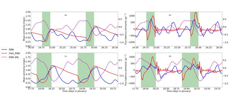
Water 2020, 12, 1945                                                                               6 of 17

concentration and hydrodynamic processes that are caused by the tide gate’s operation, the river
runoff, and ammonia loading were assigned with a constant value. The runoff is 8 m3 s−1 and
the ammonia concentration of the mainstream is 2 mg L−1 . Together with inputs from tributaries,
loading of ammonia is 137.73 g s−1 in scenario runs, which represents the expected condition after
environmental measures are fully implemented. In reality, the operation of the tide gate is decided
considering many factors besides the tidal phase. However, in the scenario runs, the opening of the tide
gate in the non-tide-receiving scenario is arranged during the ebb phase in the dominating high tide,
suggested by the Shantou Water Affairs Bureau.
      Two scenarios were designed to evaluate the impacts of tide receiving. One was run with the tide
gate opening for the whole period, which is called the tide-receiving scenario. In the other scenario,
the tide gate was operated during the ebb–tidal phases, which was called the non-tide-receiving scenario.

2.4. Analysis Methods
     Following the method proposed by Lerczak et al. and Zhou et al. [36,37], the transport of ammonia
is decomposed into a seaward advection due to net outflow, estuarine transport with seaward flow at
surface and landward flow near the bottom, and tidal oscillation.
                             Z
                       Ns ≈ h (u0 N0 + ue Ne + ut Nt )dAi = Q f N0 + Fe + Ft                       (1)

      The component with subscript t varies predominantly on tidal scales. While components with
subscript 0 and ε vary on subtidal time scales. Angled brackets indicate a low-pass, subtidal temporal
filter, of which the details are described in [38].
      To quantify the extent to which the water column is stratified, the stratification index (N) is
calculated based on the difference in salinity between bottom and surface:

                                                         δS
                                                   N=                                                 (2)
                                                         S0

where the S0 is the vertically averaged salinity and the δS is the difference in salinity between surface
and bottom. The water column is mixed when N < 0.1. When N is in the range of 0.1–1, the water
column is determined as partially mixed. When the N is higher than 1, there is evident stratification
resulted from salty water intrusion.
      Model results were evaluated quantitatively using 2 skill metrics, namely correlation coefficient
(r) and simulation skills (SS) defined by Warner et al. [39]. In Equations (3) and (4), X is the variable
and X is the corresponding mean value. Better agreement between model results and observations
will yield a skill approaching one, and vice versa.
                                      PN
                                        i=1 (Xmod − Xmod )(Xobs − Xobs )
                           r=                                                                         (3)
                                                      2 PN                 2 1/2
                                [ N
                                 P
                                   i=1 (Xmod − Xmod )    i=1 (Xobs − Xobs ) ]
                                                   PN
                                                     i=1 |Xmod   − Xobs |2
                             SS = 1 − PN                                                              (4)
                                          i=1   (|Xmod − Xmod | + |Xobs − Xobs |)

3. Results

3.1. Validation
     Surface elevation has been sampled since November 2019, in two monitoring stations located
200 m upstream and downstream to the HMB tide gate, respectively, with a temporal interval of
4 h. In the upstream station, ammonia has also been monitored. After data quality control and
checking for data continuity of input variables, such as the record of tide gate operation, ammonia,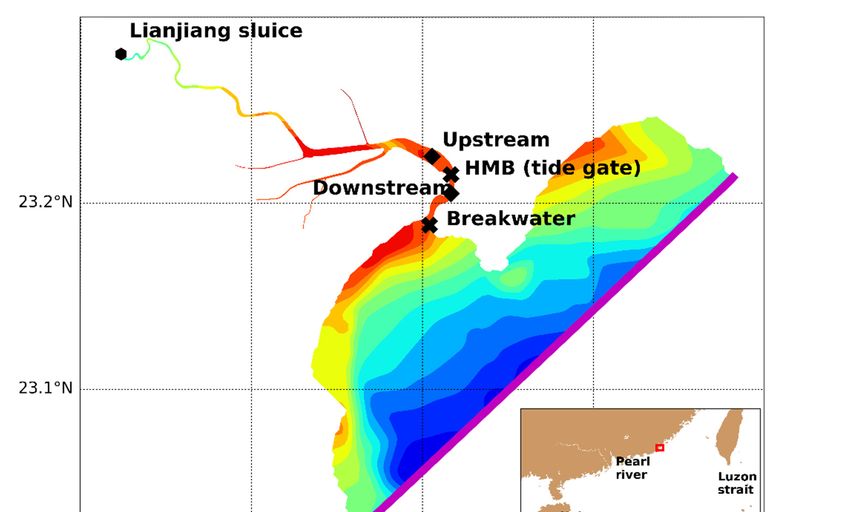
is shown in Figure 2 and quantified model skill results are listed in Table 1.

       Table 1. Statistical summary of the difference between observation and results of the simulation,
       using correlation coefficient (r) and model skills (SS).

Water 2020, 12, 1945                                               Time                      7 of 17
                        Variable       Station       2020.1.4–1.7 2020.1.24–1.27
                                                        r      SS       r     SS
and runoff in upstream, observed data from 4–7th and 24–28th in January were selected to represent
                       Elevation      HMB     up      0.87    0.96    0.89   0.95
hydrodynamic and biochemical conditions in neap/spring tidal phase. The result of the comparison is
                       Elevation model
shown in Figure 2 and quantified    HMB skilldown
                                              results 0.85    0.93
                                                      are listed      0.901.
                                                                 in Table    0.95
                       Ammonia        HMB up          0.20 0.38       0.41   0.15

        Figure 2. Comparison between simulation results and observed data. Water surface elevation in the
      Figure 2. Comparison between simulation results and observed data. Water surface elevation
        upstream (a, b) and downstream (c, d) part of the HMB tide gate were plotted in the first and second
      in the upstream (a,b) and downstream (c,d) part of the HMB tide gate were plotted in the first and
        row. Fluctuations of ammonia were shown in the last row (e, f). Time series of neap and spring
      second row. Fluctuations of ammonia were shown in the last row (e,f). Time series of neap and spring
        phases were arranged in the left and right panel, respectively.
      phases were arranged in the left and right panel, respectively.

      The 1.
     Table simulation     is able toofcapture
              Statistical summary               the basic
                                        the difference      fluctuation
                                                         between        of ammonia
                                                                 observation           and
                                                                             and results     surface
                                                                                         of the      elevation,
                                                                                                simulation, usingwhich
 are correlation
     influencedcoefficient
                   by the amount       of input
                              (r) and model  skillsin(SS).
                                                       the upstream and modulated by tide gate operation and
 propagation of tidal waves. When the tide gate was closed, the river runoff accumulated in the
                                                              Time
 upstream of the HMB and water surface was gradually elevated      (Figure 2a, b). When the tide gate
                                   Station
 was open, the tidalVariable
                      oscillation was detectable 2020.1.4–1.7     2020.1.24–1.27
                                                  also in the upstream     part. The ammonia in the
                                                          r        SS         r        SS
                        Elevation       HMB up           0.87      0.96      0.89      0.95
                        Elevation      HMB down          0.85      0.93      0.90      0.95
                        Ammonia         HMB up           0.20      0.38      0.41      0.15

      The simulation is able to capture the basic fluctuation of ammonia and surface elevation, which
are influenced by the amount of input in the upstream and modulated by tide gate operation and
propagation of tidal waves. When the tide gate was closed, the river runoff accumulated in the upstream
of the HMB and water surface was gradually elevated (Figure 2a,b). When the tide gate was open,
the tidal oscillation was detectable also in the upstream part. The ammonia in the upstream part also
experienced an increase after tide receiving, mainly due to the transport of ammonia from the further
upstream part where industrial and domestic sewage was discharged into the river. However, there are
discrepancies in the ammonia concentration which mainly originated from boundary conditions. First,
there were omissions in the records of operation of the tide gate. Even though these omissions did
not happen in the time series which we used here, the influence on the transport and transformation
of nitrogen in the whole simulation could not be excluded. Second, the loading of river runoff,
nitrogen, and other contaminants from other tributaries was prescribed by constant values due to
lacking continuous observations. This could contribute to the discrepancy of the definite amplitude
of ammonia. However, the simulation is able to reflect the major variation in the hydrodynamic and
biochemical processes, which depends on reasonable parameters’ setting and reliable boundary forcing.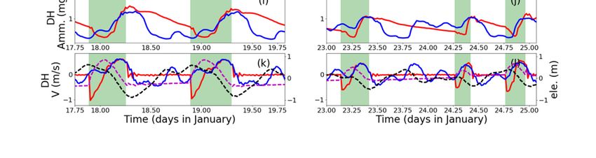
Water 2020, 12, 1945                                                                                            8 of 17

3.2. Variation of Ammonia Concentration
      Given the improved sea–river connection under the identical inputs of ammonia load and river
runoff, the concentration in the upstream part of the river has been reduced (Figure 3a–c). The descend
range decreased gradually from upstream to downstream, from 0.64 mg L−1 to 0.15 mg L−1 (Figure 3c).
The proportion of reduction shows the highest value in the downstream part near the breakwater (40%)
(Figure 3d). The downstream portion relative to HMB experienced a relatively marginal reduction
of 22% (Figure 3d). The most contaminated area is located in the north-eastern direction of the UD
cross-section, with an ammonia concentration of 1.4 mg L−1 in the tide-receiving scenario (Figure 3a)
and 2.0 mg L−1 in the non-tide-receiving scenario (Figure 3b). The portion within around 1 km north
to HMB, enveloped by the contour line of 1.0 mg L−1 and 1.4 mg L−1 in the tide-receiving (Figure 3a)
and non-tide receiving (Figure 3b), indicates an inburst of water intrusion from HMB, which results
in a dilution of ammonia concentration. However, in the downstream portion relative to the HMB,
the reduction of ammonia is limited to less than 0.3 mg L−1 (Figure 3c). The strong tidal mixing
homogenizes
Water             the spatial
      2020, 12, x FOR         variation of reduction in the downstream. Nevertheless, the closer to the
                      PEER REVIEW                                                                       river
                                                                                                      9 of 20
                                                                                   −1
mouth, the less amplitude of reduction is displayed, decreasing from 0.3 mg L close to the HMB to
0.15 mg L−1 near the breakwater (Figure 3c).

      Figure 3. The averaged ammonia concentration for a spring–neap tidal cycle in the tide-receiving
      scenario (a), non-tide-receiving scenario (b), and the comparison between the two scenarios
      (tide-receiving
     Figure            scenario-ammonia
              3. The averaged    non-tide-receiving scenario)
                                          concentration for a (c). The relative
                                                              spring–neap       change
                                                                             tidal cycle proportion  is plotted
                                                                                         in the tide‐receiving
      in (d) (tide-receiving scenario minus non-tide-receiving scenario)/non-tide-receiving   scenario).
     scenario (a), non‐tide‐receiving scenario (b), and the comparison between the two scenarios
     (tide‐receiving scenario‐ non‐tide‐receiving scenario) (c). The relative change proportion is plotted in
3.3. Variations in Time Series
     (d) (tide‐receiving scenario minus non‐tide‐receiving scenario)/non‐tide‐receiving scenario).
       As shown in Figure 3, the reduction in ammonia shows different amplitudes and spatial variabilities.
3.3. Variations  in Time
 To further resolve   the Series
                          key processes responsible for spatial and even temporal variability, time series of
 three typical cross-sections, which represent the upstream portion (UH), the downstream portion (DH)
      As shown in Figure 3, the reduction in ammonia shows different amplitudes and spatial
 relative to HMB, and the HMB tide gate were selected for further investigations of the time series related
variabilities. To further resolve the key processes responsible for spatial and even temporal
 to tidal cycle and the operation of the tide gate (Figure 4). The time series of averaged concentration of
variability, time series of three typical cross‐sections, which represent the upstream portion (UH),
 ammonia and flux balance in the downstream part (from HMB to breakwater) are resolved in Figure 5.
the downstream portion (DH) relative to HMB, and the HMB tide gate were selected for further
 The spatial extent and duration of variations in ammonia concentration caused by tide-receiving are
investigations of the time series related to tidal cycle and the operation of the tide gate (Figure 4).
The time series of averaged concentration of ammonia and flux balance in the downstream part
(from HMB to breakwater) are resolved in Figure 5. The spatial extent and duration of variations in
ammonia concentration caused by tide‐receiving are revealed in a Hovmöller diagram built along
the downstream part of the river, covering spring–neap cycles (Figure 6). In Figure 6, data have been
weighted averaged in each cross‐section along the river. The spatial upper limit of this diagram is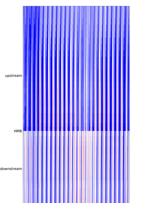
Water 2020, 12, 1945 9 of 17
revealed in a Hovmöller diagram built along the downstream part of the river, covering spring–neap
cycles (Figure 6). In Figure 6, data have been weighted averaged in each cross-section along the river.
TheWater
spatial
2020, upper limit
12, x FOR PEERof this diagram is the last tributary close to the river mouth.
REVIEW 10 of 20
Figure 4. Time series of velocity and ammonia concentration in 3 cross-sections: downstream part
relative
Figureto4.HMB
Time(UH)series(a–d), HMB and
of velocity tide ammonia
gate) (e–h), and downstream
concentration part relativedownstream
in 3 cross‐sections: to HMB (DH) (i–l)
part
(Figure 1). to
relative TwoHMB semi-diurnal
(UH) (a–d),cycles,
HMB tidein the spring
gate) phase
(e–h), and (17.75th–19.75th
downstream partof January)
relative and neap
to HMB (DH)phases
(i–l)
(23rd–26nd
(Figure 1).ofTwo
January), were plotted
semi‐diurnal cycles, inonthe
thespring
left panels
phase and right panels.ofValues
(17.75th–19.75th January)in and
the tide-receiving
neap phases
scenario were plotted in blue curves and the non-tide-receiving scenario in red curves,
(23rd–26nd of January), were plotted on the left panels and right panels. Values in the tide‐receiving with tide gate
opening periods marked out by green shadows. Tidal elevations of HMB were
scenario were plotted in blue curves and the non‐tide‐receiving scenario in red curves, with
Water 2020, 12, x FOR PEER REVIEW plotted together with
tide gate 12 of 20
velocity to show
opening periodsthemarked
tidal phases
out by(c,green
d, g, shadows.
h, k, l). For velocity,
Tidal seaward
elevations is a positive
of HMB valuetogether
were plotted and vicewith
versa.
velocity to show the tidal phases (c, d, g, h, k, l). For velocity, seaward is a positive value and vice
versa.
The opening of the tide gate in the non‐tide‐receiving scenario is arranged in the falling of
high‐high water in each daily cycle. In the non‐tide‐receiving scenario, when the tide gate is closed,
water bodies in the upstream part is blocked from the downstream and experiences gradually
increasing of the ammonia value (Figure 4a,b,e,f). After the tide gate is opened, the concentration in
the upstream increases and drops down in the first half of the opening period and then increases
again. The concentration returns to the prior level after the closing of the tide gate in 2–3 h in the
neap phase (Figure 4b,f) and in around 6 h in the spring phase (Figure 4a,e). Without the modulation
of the tide gate, in the tide‐receiving scenario, the water body mainly fluctuates with tidal velocities,
which brings the water body with high ammonia value seaward in the ebb phases and transport
Figure 5. The averaged concentration of ammonia in the cross-section between the HMB (tide gate)
water body
Figurefrom downstream
5. The with lower of
averaged concentration concentration
ammonia in the landward during
cross‐section flood the
between phases.
HMB The (tidetide‐
gate)or
and breakwater in the neap (a) and spring phase (c). The balance of ammonia flux (seaward flux
tide‐gate‐regulated
and breakwater oscillation
in the neapin (a) ammonia concentration
and spring phase is more
(c). The balance evidentflux
of ammonia in(seaward
the spring phase
flux from
from HMB minus seaward flux from breakwater) during the neap (b) and spring (d) phase. Seaward
(Figures 4a,e,iminus
HMB and 5c) than influx
seaward thefrom
neapbreakwater)
tide (Figures 4b,f,jthe
during and 5a).(b) and spring (d) phase. Seaward
neap
transportation is a positive value. Concentrations andandfluxflux
of ammonia in in
the tide-receiving scenario
When the tide
transportation gate is opened
is a positive in Concentrations
value. the non‐tide‐receiving ofscenario
ammoniaduring the spring phase,
the tide‐receiving scenariothe
are in are
blueinand non-tidal scenario in red. Water surface elevation is also plotted in dash lines in magenta
water body floods landward from the tide gate in the HMB (Figure 4g) and the ammonia
blue and non‐tidal scenario in red. Water surface elevation is also plotted in dash lines in
to indicate the to
tidal phase. theThe
magenta
concentration indicate
decreases from 2.2tide
tidal mg gate
phase. opening
L−1The
to around period
tide gate
0.5 is marked
opening
mg L−1 in 2 out
period by the out
his(Figure
marked green
4e).byInshadow.
the
thegreen
latershadow.
period of
the opening‐gate operation, the HMB experiences an increase in the ammonia concentration, which
is resulted from seaward transport of the polluted water body from the further upstream part. The
landward intrusion in the first half of the tide opening period is not only predominant in the
upstream part relative to the HMB, but also in the downstream part (Figure 4k). The negative flux of
Water 2020, 12, 1945                                                                                                 10 of 17
  Water 2020, 12, x FOR PEER REVIEW                                                                                    13 of 20

     Figure
       Figure6. 6.Hovmöller
                   Hovmöllerdiagram
                                diagramofofthethe
                                                difference
                                                  difference (tide-receiving
                                                                (tide‐receiving scenario
                                                                                   scenariominus
                                                                                              minusnon-tide-receiving
                                                                                                       non‐tide‐receiving
     scenario)  in the concentration  of ammonia     along   the  river.  The  x-axis
       scenario) in the concentration of ammonia along the river. The x‐axis representsrepresents   thethe
                                                                                                        time  evolution
                                                                                                           time evolution
     and
       and    y-axis
         thethe      depicts
                 y‐axis      thethe
                        depicts  location  along
                                    location      thethe
                                              along    river.  The
                                                          river. Thetide  elevation
                                                                       tide          is plotted
                                                                             elevation           in in
                                                                                        is plotted  thethe
                                                                                                         lower panel
                                                                                                           lower     to to
                                                                                                                 panel
     identify tidal phases.
       identify tidal phases.

      The opening of the tide gate in the non-tide-receiving scenario is arranged in the falling of
   4. Discussion
high-high water in each daily cycle. In the non-tide-receiving scenario, when the tide gate is closed,
         Concerning
water bodies    in the theupstream
                            ammoniapartflux is
                                            compromised
                                               blocked from   by the
                                                                  different transportand
                                                                       downstream     processes  that aregradually
                                                                                          experiences      quantified
   by Equation   (1), the  tidal oscillation plays  the  dominant     role and shows  the spring–neap
increasing of the ammonia value (Figure 4a,b,e,f). After the tide gate is opened, the concentration      fluctuation.
in The  instantaneous
    the upstream         ammonia
                   increases         flux driven
                               and drops    downby in the
                                                       the tide
                                                            first(140
                                                                  half Ton/spring–neap  cycle)and
                                                                       of the opening period   is around    one order
                                                                                                   then increases
   larger than that transported by river net‐flow and estuarine circulation (15 Ton/spring–neap cycle,
   Figure 7c, d). Even though the tidal oscillation flux has been modulated by the operation of the tide
Water 2020, 12, 1945 11 of 17
again. The concentration returns to the prior level after the closing of the tide gate in 2–3 h in the neap
phase (Figure 4b,f) and in around 6 h in the spring phase (Figure 4a,e). Without the modulation of
the tide gate, in the tide-receiving scenario, the water body mainly fluctuates with tidal velocities,
which brings the water body with high ammonia value seaward in the ebb phases and transport
water body from downstream with lower concentration landward during flood phases. The tide-
or tide-gate-regulated oscillation in ammonia concentration is more evident in the spring phase
(Figure 4a,e,i and Figure 5c) than in the neap tide (Figure 4b,f,j and Figure 5a).
When the tide gate is opened in the non-tide-receiving scenario during the spring phase, the water
body floods landward from the tide gate in the HMB (Figure 4g) and the ammonia concentration
decreases from 2.2 mg L−1 to around 0.5 mg L−1 in 2 h (Figure 4e). In the later period of the opening-gate
operation, the HMB experiences an increase in the ammonia concentration, which is resulted from
seaward transport of the polluted water body from the further upstream part. The landward intrusion
in the first half of the tide opening period is not only predominant in the upstream part relative to
the HMB, but also in the downstream part (Figure 4k). The negative flux of ammonia (landward)
in the first half of the tide gate opening period and positive flux (seaward) in the second half of the tide
gate opening period are also visible in the flux balance in the downstream portion (Figure 5b,d).
Compared to the regular and obvious change along tidal cycle in the spring phase (Figure 4e,g),
during the neap phase, the asymmetry of the semi-diurnal tide in a lunar day decreases, which results
in less distinction between higher-high tide, lower-high tide and associated tidal currents (Figure 4d,h,l).
The basic variation pattern, i.e., a decrease in ammonia concentration due to landward intrusion of
seawater and an increase in ammonia after the currents shifts seawater still holds for the neap phase.
However, because of the comparably weaker seawater intrusion in the neap tide, the amplitude of
response in ammonia concentration is smaller in neap tide (no more than 0.5 mg L−1 decreased by tidal
cycle and around 0.75 mg L−1 by the operation of tide gate; Figure 4b,f,j and Figure 5a) than spring tide
(around 1mg L−1 driven by tidal cycle or the operation of tide gate; Figure 4a,e,i and Figure 5c).
Besides the similar pattern of the responses of velocity and ammonia concentration in the tide gate
opening period, the most distinct pattern between the upstream and downstream parts in the non-tide
scenario occurs when the tide gate is closed. At the end of the tide gate opening period, the ammonia
concentration at the UB reached 1.75 mg L−1 , which continues its increase for 3 h after the close of
the tide gate (Figure 4a,b,e,f). It maintains a high level of around 2.5 mg L−1 until the next re-opening of
the tide gate. In the downstream part, on the contrary to the situation of upstream which experienced
an accumulation of ammonia in the tide gate closing period, the DH receives dense ammonia flux
in the second half of the tide gate opening period and recover better water quality in the rest part of
a tidal cycle (Figure 4i,j).
Comparing the ammonia concentration between two scenarios, we found that in most part of
the time period, the water quality in the tide-receiving scenario is better than the non-tide-receiving
scenario, which is in agreement with the averaged pattern for a spring–neap cycle (Figure 3c). However,
there are some exceptional conditions when the water quality deteriorates after the tide receiving.
In the UH site, the ammonia concentration is lower in the tide-receiving scenario except for the period
when the reduction of ammonia concentration after the tide gate opening reaches the maximum
(around 18 and 19 January) in the spring phase (Figure 4a,e). This phenomenon lasts for 2–3 h
during the spring phase and could cover the spatial range from the breakwater to the UH section
(Figure 6). This may be also associated with the lower averaged concentration spatially contoured by
1.13 mg L−1 (Figure 3a) and 1.4 mg L−1 (Figure 3b), which depicts the spatial coverage of the obvious
landward intrusion of seawater. Compared to the spring phase, a weaker landward intrusion
and consequential limited reduction of ammonia concentration in the neap phase around the UH
cross-section (Figure 6). The reduction is limited and the ammonia concentration in the non-tide
scenario stays higher in the further UH (Figure 4b). On the contrary, in the downstream part, during
the neap tide, the duration time when the ammonia concentration in the tide-receiving scenario is
higher could last for around half a day at the DH site (Figure 4j, 23.8–24.4 d, January) and otherWater 2020, 12, 1945 12 of 17
downstream portions (Figure 6). The several peaks in the ammonia concentration time series coincide
with the seaward flow (Figure 4l) and seaward flux of ammonia (Figure 5b) input from HMB, which
indicates back–forth oscillation of water body with higher ammonia concentration in the neap tide.
4. Discussion
Concerning the ammonia flux compromised by different transport processes that are quantified
by Equation (1), the tidal oscillation plays the dominant role and shows the spring–neap fluctuation.
The
Waterinstantaneous
2020, 12, x FOR PEERammonia
REVIEWflux driven by the tide (140 Ton/spring–neap cycle) is around 14 one
of 20
order larger than that transported by river net-flow and estuarine circulation (15 Ton/spring–neap
gate, i.e.,
cycle, little
Figure landward
7c,d). Even flux when
though thethe tideoscillation
tidal gate is closed in the
flux has non‐tide‐receiving
been modulated by the scenario (Figure
operation of
7b),tide
the for gate,
a spring–neap cycle, the flux
i.e., little landward accumulative
when the tidefluxes areiscomparable
gate closed in thebetween two scenarios
non-tide-receiving with a
scenario
decrease
(Figure of for
7b), around 8 Ton in the
a spring–neap tide‐receiving
cycle, scenario.
the accumulative The are
fluxes tidecomparable
oscillation transport
between is undermined
two scenarios
during
with the neapof
a decrease phase,
aroundwhich
8 Toncaninbethe
verified by the moderate
tide-receiving scenario.sloping of accumulative
The tide flux driven
oscillation transport is
by tide during
undermined duringthe the
neap phase
neap (24–25th
phase, whichof canJanuary, Figure
be verified 7a,b).
by the Duringsloping
moderate the neap phase, in the
of accumulative
non‐tide‐receiving
flux driven by tide during scenario,thethe seaward
neap phasetransport ammoniaFigure
(24–25th of January, is intensified duringthe
7a,b). During theneap
neapphase,
phase
(Figure
in 7d), which is induced
the non-tide-receiving scenario,by thethe enhanced
seaward stratification
transport of ammonia(Figure 8). However,
is intensified duringthis
theis not
neap
detectable
phase (Figurein the
7d),tide‐receiving
which is inducedscenario.
by the enhanced stratification (Figure 8). However, this is not
detectable in the tide-receiving scenario.
Figure 7. Ammonia flux resulting from tidal oscillation (red line), subtidal estuarine circulation
Figure 7.dash
(magenta Ammonia
line), netflux resulting
outflow (greenfrom tidal
line) in the oscillation (red
tide-receiving line), subtidal
scenario (d) and theestuarine circulation
non-tide-receiving
scenario(c). Accumulative flux since the 10 January for the non-tide-receiving scenario is and
(magenta dash line), net outflow (green line) in the tide‐receiving scenario (d) the
plotted
non‐tide‐receiving scenario(c). Accumulative flux since the 10 January for
in (a) and tide-receiving scenario in (b). A positive value indicates an oceanward flux. the non‐tide‐receiving
scenario is plotted in (a) and tide‐receiving scenario in (b). A positive value indicates an oceanward
flux.predominant contribution from tidal oscillation transport and elevated flux during spring
The
phase are not well in line with the phenomenon observed in other estuary systems, such as Modaomen
EstuaryThe[37]
predominant
and Hudson contribution
River Estuary from tidal
[40], oscillation
where transport
salty water and elevated
intrusion flux during
and material spring
transport are
phase are not well in line with the phenomenon observed in other estuary
more prevalent in the neap phase. In those cases, the stratification is further enhanced in the neap systems, such as
Modaomen
tide and hence Estuary [37] andsalty
aggravating Hudson
waterRiver Estuary
intrusion from [40],
thewhere
bottom salty water intrusion
landward and fluvial and material
materials
transport are more prevalent in the neap phase. In those cases, the stratification
on the surface layer transport seaward [41]. In the Lianjiang River, the major part of the downstream is further enhanced
in the neap
portion tide andmixed,
is partially hence aggravating
except for a saltyshortwater
period intrusion
during from
the ebb the phase
bottom(Figure
landward and Given
8e–h). fluvial
materials
the limited onriver therunoff,
surface layer and
shallow transport seaward
flat estuary shape[41].
andInweak
the Lianjiang River,
stratification, the the major of
transport part of the
material
downstream portion is partially mixed, except for a short period during the
is mainly driven by tide oscillation instead of net outflow and estuary circulation.That is also why ebb phase (Figure 8e–h).
Given
the tidalthe limited river
frequency runoff, shallow
is predominant and
in the flat estuary
variation shape andconcentration
of ammonia weak stratification,
(Figurethe transport
4) and flux
of material is mainly driven by
(Figure 5) in the estuary part of the river.tide oscillation instead of net outflow and estuary circulation.That is
also why the tidal frequency is predominant in the variation of ammonia concentration (Figure 4)
and flux (Figure 5) in the estuary part of the river.Water 2020, 12, 1945 13 of 17
Water 2020, 12, x FOR PEER REVIEW 15 of 20
Figure 8. Time series of stratification index N (calculated by Equation (2)) in 4 cross-sections: UH
Figure 8. Time
(a,b); HMB series
(c,d); DHof(e,f)
stratification index N
and breakwater (calculated
(g,h). by Equation (2))of
Spring (17.75th–19.92th inJanuary)
4 cross‐sections:
and neapUH (a,
phases
b);(23rd–25.07th
HMB (c,d); DH (e,f) and breakwater (g,h). Spring (17.75th–19.92th of January) and neap phases
of January), which contain 2 semi-diurnal cycles, were plotted on the left panels and right
(23rd–25.07th of
panels. Values in January), which contain
the tide-receiving 2 semi‐diurnal
scenario were plottedcycles,
in bluewere plotted
curves onthe
and in thenon-tide-receiving
left panels and
right panels. Values in the tide‐receiving scenario were plotted in blue curves
scenario in red curves, with the tide gate opening period marked out by green shadows. Tidal andelevations
in the
non‐tide‐receiving scenario in red curves, with
of HMB were plotted to show the tidal phases (c,d). the tide gate opening period marked out by green
shadows. Tidal elevations of HMB were plotted to show the tidal phases (c, d).
In this study, the distribution of ammonia was mainly attributed to physical transport and mixing.
In this study,processes,
Biogeochemical the distribution
such as of ammonia was
nitrification, mainly attributed
denitrification [42], andto physical transport
consumption by algaeand [43],
mixing.
may also be responsible for the transform of ammonia [44], but account for limited proportion in by
Biogeochemical processes, such as nitrification, denitrification [42], and consumption this
algae
case.[43],
The may
limitedalsobiogeochemical
be responsibletransformation
for the transform of ammonia[44]
of ammonia , but account
can be verified by the for limited
relationship
proportion in thisand
between salinity case. The limited
ammonia biogeochemical
(Figure transformation
9). If a linear relationship existsofbetween
ammonia can be verified
a dissolved by
constituent
the relationship between salinity and ammonia (Figure 9). If a linear
and salinity which is a conservative indicator of mixing between seawater and freshwater, then relationship exists between a
dissolved constituent
the dissolved constituent and can
salinity which isas
be described a conservative
conservativein indicator
this mixing of mixing
process. between seawater holds
This assumption and
freshwater,
approximately theninthe thedissolved constituent
tide-receiving scenario canin be
thedescribed
downstream as conservative
portion relative in to
this
UH.mixing process.
The correlation
This assumption
between salinity holds approximately
and ammonia fluctuates in around
the tide‐receiving value < in
−0.75, with pscenario theindicating
0.01, downstream portion
that removing
relative to UH.
or addition ofThe correlation
ammonia between
is often salinityminor
a relatively and ammonia fluctuatesthe
process affecting around −0.75, with
distribution P valueto
compared
< physical
0.01, indicating that removing or addition of ammonia is often a relatively
dilution. In both scenarios, the R value increases in the upstream portion relative to HMB. minor process affecting
the
Thedistribution
curve for the compared to physical
tidal scenario dilution.near
also increases In both scenarios,
the river mouththe R value increases
(breakwater), in the
which indicates
upstream portion relative
that the back-force to HMB.
oscillation caused Thebycurve
tide mayfor the tidal
result in scenario also increases
longer residual time fornear the river
ammonia near
mouth
the river mouth and allow other biogeochemical processes to take part in. This is also suggestedinby
(breakwater), which indicates that the back‐force oscillation caused by tide may result
longer residual
the budget time forthat
calculation ammonia
the netnear the river
exported mouthflux
ammonia andinallow other biogeochemical
the tide-receiving scenario isprocesses to
less than that
take part
in the in. This is also suggested
non-tide-receiving scenario by the budget
(Table calculation
2). Furthermore, thethat the net exported
correlation ammonia
is not robust in theflux in
further
the tide‐receiving
upstream portionscenario
relativeistoless
the than that in
UH (data nottheshown),
non‐tide‐receiving
which indicates scenario (Table
that the 2). Furthermore,
behavior of ammonia
the
wascorrelation
subject to is not robust
in-situ uptakein orthe furtherIt upstream
removal. also suggestsportion
that therelative to the UH processes
biogeochemical (data not have
shown),
to be
which indicates that the behavior of ammonia was subject to in‐situ
taken into account if we aim at giving a further quantitative explanation of ammonia or even total uptake or removal. It also
suggests
nitrogen’s that the biogeochemical
budget with more in situ processes
measurements.have to be taken into account if we aim at giving a
further quantitative explanation of ammonia or even total nitrogen’s budget with more in situ
measurements.Water 2020, 12, x FOR PEER REVIEW 16 of 20
Water 2020, 12, 1945 14 of 17
Figure
Figure 9. 9.
TheThe correlation
correlation between
between salinity
salinity and and ammonia
ammonia nitrogen
nitrogen alongalong thefrom
the river riverbreakwater
from breakwater
until
until
the UH the UH cross‐section.
cross-section. The Rofvalues
The R values of and
the tide the non-tide-receiving
tide and non‐tide‐receiving
scenarios scenarios
are plottedare
in plotted
red andin
red respectively.
blue, and blue, respectively. P lower
p values are valuesthan
are lower
0.01. than 0.01.
Table Seaward flux ofof
The2.consequences ammonia andtide
different water mass
gate at the cross-section
operations of HMBand
are mainly breakwater
evaluated by thein dilution
both of
scenarios for a lunar cycle in the spring/neap phase and for a spring–neap cycle.
ammonia concentration. However, there are varieties of criteria for evaluations of the operation
planning which would be considered in the
Concerned Timefuture.
Period With elevated water storage in the river
Spring–Neap Cyclein the
Sections Variable Neap Tide Non-Tide
tide‐receiving scenario, the dense Spring ammonia Tide has Non-Tide
been diluted. The decreased ammonia Tide isNon-Tide
expected to
benefit theAmmonia
recovery FluxofSeaward
the ecological function
(Ton/Lunar Cycle) of the Lianjiang River. Particularly in the
(Ton/Spring–Neap dry season
Cycle)
HMB
when the storage of water in the Lianjiang 10.52 River 13.15
is much lower 4.52 than the 8.56necessary126.23ecological
165.65water
Breakwater 10.85 10.45 6.74 7.93 135.52 144.46
demand. The Flux advantage
Seaward with more (104 available water storage is well beyond
m3 /Lunar Cycle) mere considering
(104 m3 /spring–neap cycle) a
HMB
decrease of pollutants. Even though the water 379.86
196.77 storage has been elevated,
−40.08 361.46 due to the 16,565.13
12,623.16 back–forth
Breakwater 219.34 146.91 −66.88 200.89 13,551.69 14,446.32
currents in the tide‐receiving scenario, the total exported amount of ammonia decreased by 6% at the
cross‐section of the breakwater and 23% at the HMB (Table 2). The downsteam part relative to HMB
The consequences
experiences higher of different tide gate
concentration duringoperations
neap are mainly
tides. In evaluated
this regard, by the dilution
the of ammonia
advantage of the
concentration.
tide‐receivingHowever,
scenario,therewithareno varieties of criteria
control over for evaluations
the natural flow, hasoftothe be operation
reconsidered,planning whichof
in aspects
would be considered
the flux in the future.
of total nitrogen, residualWith
timeelevated water storage
of pollutants and so in on.theIt river in the
is worth tide-receiving
noting scenario,of
that the increase
the dense ammonia
ammonia has been
concentration, or diluted. The decreased
longer duration ammoniaammonia
of higher‐level is expected in theto benefit
downstreamthe recovery
relativeofto
the ecological function of the Lianjiang River. Particularly in the dry
the HMB may influence aquatic agriculture. In the future study, according to varied standardsseason when the storage of wateror
intargets
the Lianjiang River is much
of environmental lower thana the
protection, necessary
variety ecological should
of evaluations water demand.
be further Theexplored,
advantagesuch withas
more available
residual time water storage is
of pollutants, well beyond
duration mere considering
of high‐level concentration a decrease of pollutants.
of specific constituents, Evenand though
export
the water
flux storage has been elevated, due to the back–forth currents in the tide-receiving scenario,
of contaminants.
the total exported amount of ammonia decreased by 6% at the cross-section of the breakwater and 23%
at the HMB
Table (Table 2). The
2. Seaward fluxdownsteam
of ammoniapart and relative
water mass to HMB
at theexperiences
cross‐sectionhigher
of HMBandconcentration
breakwater during
in
both scenarios
neap tides. for a lunar
In this regard, cycle in theof
the advantage spring/neap phase and
the tide-receiving for a spring–neap
scenario, cycle. over the natural
with no control
flow, has to be reconsidered, in aspects of the flux of total nitrogen, residual time of pollutants and so
on. It is worth noting that the increase Concerned of ammonia Time Period
concentration, Neapor longer duration of higher-level
Spring–Neap Cycle
Sections Variable Spring Non‐Tide
ammonia in the downstream relative to the HMB may influence
Non‐Tide aquatic agriculture. In the future
Tide
Tide Tide Non‐Tide
study, according to varied standards or targets of environmental protection,
Ammonia Flux Seaward (Ton/Lunar Cycle)
a variety of evaluations
(Ton/Spring–Neap Cycle)
shouldHMB be further explored, such as residual time of pollutants,
10.52 13.15 duration
4.52 of 8.56
high-level126.23
concentration
165.65 of
specific constituents, and export flux of contaminants.
Breakwater 10.85 10.45 6.74 7.93 135.52 144.46
As the first Fluxto
trial Seaward
evaluate the (104 mof
impact
3/Lunar Cycle)
modulation of the tide gate (10on
4m3/spring–neap cycle)
ammonia transport,
HMB
196.77 379.86 −40.08 361.46 12623.16 16565.13
the operation plan of the tide gate has been219.34
Breakwater
simplified to 146.91
design the non-tide-receiving
−66.88 200.89
scenario.14446.32
13551.69
For the
environmental protection practice in Lianjiang, contingency plans or affirmative action would be taken
depending
As the onfirst
many factors.
trial Even though
to evaluate the impactthe tide gate is mainly
of modulation of theplanned
tide gateto open in the ebb
on ammonia phase, for
transport, the
exporting
operationpollutants
plan of the from
tidethe
gateupstream,
has beenhowever,
simplified tide gate normally
to design would not be switched
the non‐tide‐receiving scenario.on–off
For the
environmental protection practice in Lianjiang, contingency plans or affirmative action would beYou can also read