Urbanization in India: Population and Urban Classification Grids for 2011 - MDPI
←
→
Page content transcription
If your browser does not render page correctly, please read the page content below
data
Data Descriptor
Urbanization in India: Population and Urban
Classification Grids for 2011
Deborah Balk 1,2, * , Mark R. Montgomery 3,4 , Hasim Engin 1 , Natalie Lin 1 , Elizabeth Major 1
and Bryan Jones 1,2
 1   CUNY Institute for Demographic Research, City University of New York, New York, NY 10010, USA;
     hasim.engin@baruch.cuny.edu (H.E.); natalie.lin@baruch.cuny.edu (N.L.);
     elizabeth.major@baruch.cuny.edu (E.M.); bryan.jones@baruch.cuny.edu (B.J.)
 2   Baruch College Marxe School of Public and International Affairs, City University of New York,
     New York, NY 10017, USA
 3   Population Council, New York, NY 10017, USA; mmontgomery@popcouncil.org
 4   Stony Brook University, New York, NY 11794, USA
 *   Correspondence: deborah.balk@baruch.cuny.edu; Tel.: +1-646-660-6762

 Received: 6 December 2018; Accepted: 21 February 2019; Published: 26 February 2019

 Abstract: India is the world’s most populous country, yet also one of the least urban. It has long
 been known that India’s official estimates of urban percentages conflict with estimates derived
 from alternative conceptions of urbanization. To date, however, the detailed spatial and settlement
 boundary data needed to analyze and reconcile these differences have not been available. This paper
 presents gridded estimates of population at a resolution of 1 km along with two spatial renderings of
 urban areas—one based on the official tabulations of population and settlement types (i.e., statutory
 towns, outgrowths, and census towns) and the other on remotely-sensed measures of built-up land
 derived from the Global Human Settlement Layer. We also cross-classified the census data and the
 remotely-sensed data to construct a hybrid representation of the continuum of urban settlement.
 In their spatial detail, these materials go well beyond what has previously been available in the public
 domain, and thereby provide an empirical basis for comparison among competing conceptual models
 of urbanization.

 Dataset: Available at http://www.ciesin.columbia.edu/data/india-census-grids.

 Dataset License: Creative Common License CC-BY.

 Keywords: India; urbanization; population; census; built-up area; Global Human Settlement Layer;
 grid; raster

1. Introduction
      India, the world’s most populous country, is also one of the least urban. At the time of the most
recent census in 2011, 31% of the country’s population lived in urban areas according to the official
statistics [1]. Yet by other accounts, this 31% figure is far too low [2–4]. Such disagreements stem from
different conceptual models of urbanization—the higher percentages are derived from a “statistical”
perspective in which urban-ness is defined in terms of population density, areal contiguity, and the
total population of sufficiently dense contiguous areas. This approach stands in contrast to the official
classifications for India, which blend the statistical perspective with an alternative view that takes
the legal boundaries of urban jurisdictions into account. Both perspectives have merit; but it has
proven difficult to reconcile them because the data needed to do so have not been available in the
public domain.

Data 2019, 4, 35; doi:10.3390/data4010035                                       www.mdpi.com/journal/data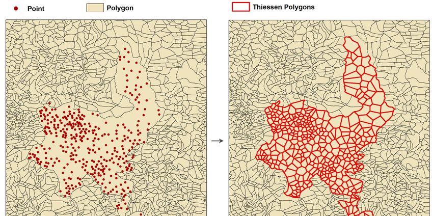
Data 2019, 4, 35                                                                                         2 of 16

     This paper places into the public domain two detailed sets of gridded estimates of urban and
rural areas at 1 km (or finer) resolution. One set is based on India’s official criteria, providing a
spatial representation of urban and rural communities as these are officially defined. The second set
of estimates is informed by the statistical perspective on urbanization, drawing on approaches that
integrate disparate data to indicate urban population [5]; these estimates extend the official criteria via
remotely-sensed measures of the density of structures, obtained from the Landsat imagery processed
by the Global Human Settlement Layer research team [6]. Taken in combination, our estimates
provide what has long been lacking: an empirical basis for a rigorous comparison of competing urban
definitions. We have made available two 2011 snapshots capturing a moment in India’s upward
trajectory of urbanization, which in the coming decades will have wide-ranging consequences for
human well-being and the natural environment [7–11]. To accompany these two urban classification
grids, we also produce a grid of population using the same finely-resolved spatial units—not previously
used as inputs in any other spatial population dataset—so that urban location and population may be
examined together.

2. Data Description
    Before describing the data collection on population and urban classifications in India that we
have produced and disseminated with this article, we should first explain the empirical ingredients.

2.1. Input Data
     Three types of data were needed to generate high-resolution grids of India’s urban areas and
population: Settlement-level demographic data from the 2011 population census; spatial boundaries
that delineate these settlements; and remotely-sensed data on built-up area. Each is described in turn.

2.1.1. Population Census Abstracts
      In a welcome departure from previous practice, India’s Office of the Registrar General and Census
Commissioner has placed into the public domain a very large collection of detailed, settlement-specific
tabulations of 2011 population census data. For the purposes of this research, the key tabulations
come in the form of what are termed primary census abstracts (PCAs)—they cover places ranging in
size from tiny rural villages to small- and medium-sized towns and upward to the largest of India’s
municipalities, providing information on the population of each settlement, its number of households,
and selected additional characteristics. Complementary spatial data—to be described below—are
available for a total of 4041 legally-constituted urban areas (statutory towns), 3893 so-called census towns,
and 640,930 rural villages. The statutory towns are further subdivided into wards, with an abstract
produced for each ward. Some of these wards are additionally designated as outgrowths.
      The four urban categories—statutory towns, wards, outgrowths, and census towns—require a
few words of explanation. Statutory towns are governed by one of the many forms of urban local
governmental authority that exist in India, with the Constitution giving considerable latitude to state
governors in decisions about whether and what type of authority to establish. The legal basis is set out
in the Constitution of India PART IXA–243Q, as follows:

      “Constitution of Municipalities. (1) There shall be constituted in every State, (a) a Nagar
      Panchayat (by whatever name called) for a transitional area, that is to say, an area in transition
      from a rural area to an urban area; (b) a Municipal Council for a smaller urban area; and
      (c) a Municipal Corporation for a larger urban area, in accordance with the provisions of
      this Part: Provided that a Municipality under this clause may not be constituted in such
      urban area or part thereof as the Governor may, having regard to the size of the area and the
      municipal services being provided or proposed to be provided by an industrial establishment
      in that area and such other factors as he may deem fit, by public notification, specify to be an
      industrial township. (2) In this article, ‘a transitional area’, ‘a smaller urban area’ or ‘a larger
Data 2019, 4, 35                                                                                     3 of 16

      urban area’ means such area as the Governor may, having regard to the population of the
      area, the density of the population therein, the revenue generated for local administration,
      the percentage of employment in non-agricultural activities, the economic importance or
      such other factors as he may deem fit, specify by public notification for the purposes of
      this Part.”

      Wards are electoral units that are overseen by statutory-urban governing bodies. There is no
automatic rule by which statutory towns and their constituent wards come into being on the basis
of well-defined demographic and economic criteria. Indeed, a notable and much commented-upon
feature of Indian urbanization has to do with the reluctance of some states to allow their large,
urban-like villages to be legally declared urban. The public finance problem is that an urban authority
may not be eligible for development funds that are earmarked for rural areas, and depending on
circumstance, state governors may be unpersuaded of the potential for obtaining commensurate
urban development funds [2–4]. These dueling political–economy considerations may well combine to
produce under-estimates of India’s urban percentages, an issue that we will investigate in what follows.
      Among all the wards of a statutory town, some can be designated as outgrowths, these being
units which hold a type of dual status. An outgrowth is an area of high-density, arguably urban
settlement that is spatially adjacent to a statutory town, and which would thus seem to be poised
on the threshold of becoming legally urban. However, outgrowths are in fact governed by rural
authorities. The ambiguous status of outgrowths is signified in their PCA identifier codes: outgrowths
are assigned both a village code and a code defining the outgrowth as a ward of the statutory town.
In India’s tabulations of urban population, outgrowths are treated as urban.
      Much like outgrowths, census towns are legally rural settlements, but they are designated as
urban for the purposes of an upcoming census and grouped with statutory urban areas in the official
post-census tabulations. The census-town designation emerges in the course of discussions between
census authorities and state government officials in the lead-up to each new census [12–14]. There
are specific demographic and socioeconomic criteria that are meant to guide the discussions, but
these criteria are evaluated on the basis of data gathered in the previous census, a practice that leaves
ample room for misunderstandings of local trends and variations in judgement [14]. Also, there is no
requirement that once classified as urban in this specialized way for a given census, a census town
must remain so classified for the next decennial census. It seems that the state-specific discussions
effectively begin anew in each census round. The census town–statutory town distinction has been in
place for many decades, and India’s system of identifier codes for settlements has long distinguished
the two.
      Our calculations reveal how important census-town designations are, for example, to the state
of Kerala’s overall percentage urban. The 2011 Census put the urban percentage of India as a whole
at 31.1 percent, with census towns accounting for only 4.2 percentage points of the total. In Kerala,
however, roughly 50.8 percent of the population is urban, a total that is well above the all-India average,
with census towns accounting for almost 29 points of this total. Indeed, had the census towns of
Kerala been ignored, only 21.9 percent of the state’s residents would have been counted as urban.
Since the status of “census town” holds only for a given census, these towns can transition from
rural village to census-urban status and then back, or alternatively can go on to become statutory
urban, a complication that spawns confusion about the longer-term meaning of India’s reported urban
percentages and which obscures the true pace of the country’s urbanization.

2.1.2. Boundary Data
     Although the PCA settlement-level tabulations have been placed in the public domain,
the government of India has not released digital records of settlement boundaries. Boundary data
must be purchased from third-party vendors, who prohibit their redistribution. We use the proprietary
“Village Map” data products (one for each state or union territory, in the WGS 1984 geographic
projection) from ML Infomap LLC to provide the vector settlement boundary input for our new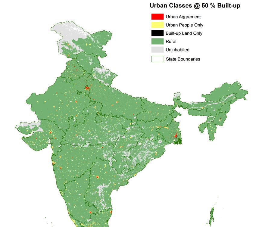
Data 2019, 4, 35 4 of 16
grids. (It is impossible to reconstitute the original boundaries from our new, gridded data products.)
According to the ML Infomap metadata, its “coastal boundaries were aligned with imagery, [with] no
gaps in polygon or no topological errors” and assure an “accuracy of the boundaries to 30–50 m”. These
spatial data include the key identifiers (indicating state, district, subdistrict, and settlement) which
(with some exceptions) allow the boundaries of each settlement to be linked to the corresponding PCA
record and thereby to the full set of PCA demographic indicators. In total, over 650,000 spatial units
have beenDataused to construct the data collection provided in this research, which represents
2018, 3, x FOR PEER REVIEW 4 of 17
more than
a 100-fold increase in the input resolution over the best publicly-available alternative, The Gridded
Populationwhichof the(with someVersion
World, exceptions) allow the [15].
4. (GPWv.4) boundaries
Althoughof eachthesettlement
settlement to boundaries
be linked to are the primarily
corresponding PCA record and thereby to the full set of PCA demographic indicators. In total, over
rendered as vector polygons, in some less populous states, settlements could only be represented in
650,000 spatial units have been used to construct the data collection provided in this research, which
terms of point locations.
represents (Implications
more than of thisinfor
a 100-fold increase theour gridding
input resolution method
over theare
bestdiscussed below).
publicly-available
Tablealternative,
1 below lists, by state
The Gridded as well as
Population forWorld,
of the IndiaVersion
as a whole, the spatial
4. (GPWv.4) inputsthe
[15]. Although that we have used in
settlement
boundaries
this research. are primarily
For statutory rendered
towns, censusas vector
towns, polygons, in some less
and villages the populous
table givesstates,
thesettlements
number of whole
could only be represented in terms of point locations. (Implications of this for our gridding method
settlements available in the spatial data. Many of these settlements are sub-divided into components
are discussed below).
that are specific Tableto1administrative
below lists, by statedistrict
as well asorforsubdistrict, butthe
India as a whole, here weinputs
spatial report only
that the used
we have total number
of settlements. Spatial For
in this research. records
statutoryfortowns,
outgrowths
census towns, are and
alsovillages
available forgives
the table the the
whole
number of of
India.
whole However,
ward-levelsettlements
spatial data available
are in the spatial
only data. from
available Many of MLthese settlements
Infomap are sub-divided
as separate into components
proprietary products. For a
that are specific to administrative district or subdistrict, but here we report only the total number of
subset of 62 cities, including all cities with a population above 1 million, we collected additional
settlements. Spatial records for outgrowths are also available for the whole of India. However, ward-
ward-levellevel
spatial
spatialinformation, as shown
data are only available fromin ML
Figure 1. Indian
Infomap cities
as separate are internally
proprietary products. organized
For a subset in a variety
of ways, andof 62as theincluding
cities, map inall Figure 1 demonstrates,
cities with a population above the1 million,
ratio ofwesettlement-level
collected additionalto ward-level units
ward-level
varies from spatial
one information,
city to the as shown
next. in Figurea1.city
Mumbai, Indianof cities
overare12internally organized in a variety
million inhabitants, consists of ways,
of two distinct
and as the map in Figure 1 demonstrates, the ratio of settlement-level to ward-level units varies from
settlements and 97 wards. Navi Mumbai, a city of just over 1 million in the Greater Mumbai region,
one city to the next. Mumbai, a city of over 12 million inhabitants, consists of two distinct settlements
is 1 settlement
and 97with
wards.89 wards,
Navi Mumbai, giving
a city it
of twice
just overthe ratio in
1 million ofthe
wards
GreatertoMumbai
settlements as1 Mumbai
region, is settlement for about
one-tenth with
of the population.
89 wards, giving itThe
twiceward-level detail
the ratio of wards reveals population
to settlements as Mumbai for and density
about variations
one-tenth of the within
cities and population. The ward-level
helps to identify detail reveals
uninhabited areaspopulation and density
(e.g., large urbanvariations
parks or within cities and
reserved land)helps
that would
to identify uninhabited areas (e.g., large urban parks or reserved land) that would otherwise skew
otherwise skew the density estimates. The distribution of population within cities is a very important
the density estimates. The distribution of population within cities is a very important factor in
factor in assessing population
assessing population exposed
exposed to spatially-specific
to spatially-specific environmental
environmental risks,flooding.
risks, for example, for example, flooding.
Data 1.for
Figure 1.Figure India
Data withwith
for India indications
indicationsfor whichcities
for which cities
we we
had had spatial
spatial ward-level
ward-level data. data.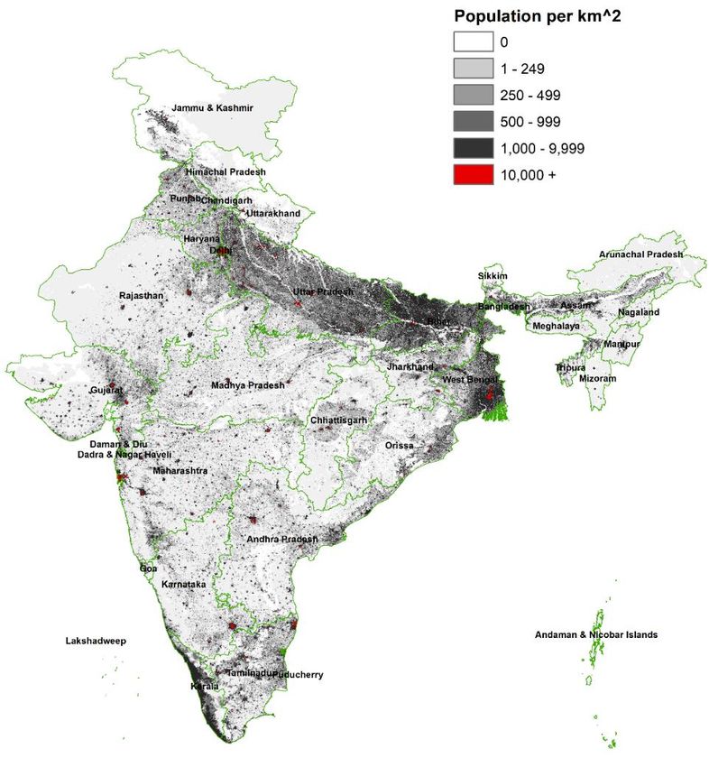
Data 2019, 4, 35                                                                                                          5 of 16

      Table 1. Overview of input vector spatial data, matched with Primary Census Abstracts: Number of
      Spatial Units by Format and Urban Classification Type.

                                                Format                   Urban Classification *
           States & Union Territories                           Statutory    Census                           Village
                                           Polygon     Point                           Ward     Outgrowth
                                                                 Town        Town
             Andamans & Nicobars               -        560          1           4        -          -          555
               Andhra Pradesh              26,927      2090        125         228      287        209        27,800
              Arunachal Pradesh                -       5616         26           1        -          -         5589
                    Assam                  22,746      4137        88          126       89        29         26,395
                     Bihar                 45,159        0         139          60       76          4        44,874
                 Chandigarh                   38         0           1          5        28         2             5
                 Chhattisgarh              18,528      2255        168          14      110         40        20,126
             Dadra & Nagar Haveli             71         0           1           5        -          -           65
                Daman & Diu                   27         0           2           6        -          -           19
                     Delhi                   256         0          3          110        -          -          112
                      Goa                    414         0          14          56        7         7           334
                    Gujarat                19,040        0         195         153      377        127        18,225
                   Haryana                  7080         0          80          74       83         15         6841
              Himachal Pradesh             13,103      7693         56           3        8         8         20,689
              Jammu & Kashmir               6766        241         86          36      232         93         6553
                  Jharkhand                32,884        0          40         188      111          1        32,394
                  Karnataka                30,232        0         220         127      459         69        29,340
                    Kerala                  1871         0         59          461      173        16          1018
                Lakshadweep                    -         27          -           6        -          -           21
               Madhya Pradesh              56,346        0         364         112      295        86         54,903
                 Maharashtra               45,926        0         256         278      898         3         43,665
                   Manipur                   493       2170         28          23        7         7          2582
                  Meghalaya                    -       6861         10          12        -          -         6839
                   Mizoram                     -        853         23           -        -          -          830
                  Nagaland                     -       1454         19           7        -          -         1428
                    Odisha                 53,283        0         107         116      171        57         51,311
                 Puducherry                  101         0           6           4        1         1            90
                    Punjab                 13,055        0         143          74      261        61         12,581
                  Rajasthan                45,287        0         185         112      291        39         44,672
                    Sikkim                   484         0           8          1         -          -          451
                 Tamil Nadu                17,450         0        721         376      373         14        15,979
                    Tripura                  917         0          16          26        -                     875
                Uttar Pradesh              108,336       0         648         267      593         63        106,774
                 Uttarakhand               16,835      293          74         41       49          19        16,793
                 West Bengal               41,482        0         129         781      286         13        40,202
                      Total                625,137    34,250      4041        3893      5265       983        640,930
      * Unpopulated spatial units are indicated by a variety of land-use types (e.g., forest, submerged areas, mountain)
      and are not indicated here. Totals for the urban classes are not mutually exclusive: for a single statutory town with
      many ward-level spatial units, the counts here include both the respective ST and wards totals. Wards also include
      outgrowths (available for all statutory towns and cities), which are also noted in separate column above, as well as
      “regular” wards (available only for selected large cities as shown in Figure 1).

     The original spatial data from ML Infomap were thoroughly cleaned and subjected to multiple
rounds of topological correction. In the course of cross-validating the ML Infomap spatial data
with census information and open-source settlement information, we uncovered numerous although
generally minor flaws in these proprietary data. As described below, we made alterations only where
necessary to achieve a match to the PCA records, and only if authoritative boundary information
lent support to the changes. (Many additional alterations could have made to the original boundary
data but were not due to inconsistencies and deficits in authoritative boundary records in India.)
Furthermore, because district-level boundary data from ML Infomap are used in other 1-km gridded
data products (such as GPW v.4), we decided to make the fewest alterations possible, systematically
adjusting only the settlement polygons that were misaligned with district or state borders.
     In particular, when we attempted to merge ward and outgrowth data from the PCAs with their
corresponding ML Infomap spatial boundaries, it became clear that some wards and outgrowths
(as well as some census towns), were either omitted from, or clearly misrepresented by, the spatial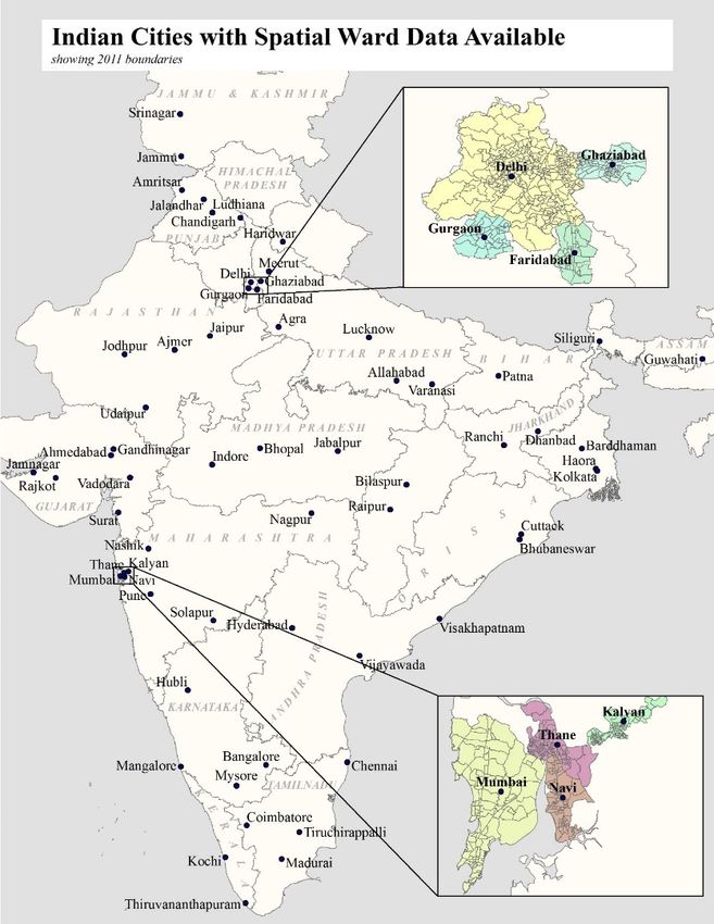
Data 2019, 4, 35                                                                                       6 of 16

data. To achieve adequate linkages, we were required to split and merge ward polygons, and needed
to draw new polygons where the omitted units could be identified with confidence. Publicly available
data, including the District Census Handbooks and Atlases [16,17] of the Indian Census, resources on
Open Street Map, and the ESRI base-map and Google were used in this data-cleaning process. In total,
over 200 new polygons were either created or substantially altered. These corrections made it possible
to achieve a match with the PCA data for nearly all of India’s settlements and outgrowths. Of the
about 1036 outgrowths identified in the PCAs, only seven have not yet been located in the spatial
boundaries data. The populations of these missing outgrowths are known, as are the statutory towns
to which they are adjacent; only their precise spatial locations are yet to be established. (Additionally, a
small number (n = 57) of outgrowths, were aggregated in the ML Infomap spatial data. Maps provided
in the Census Atlases and District Census Handbooks were not sufficiently informative to identify the
individual outgrowth boundaries, leaving us no option but to aggregate, the PCA records to match the
ML Infomap spatial units (n = 11).)
      The ward-level spatial data supplied by ML Infomap for Delhi, New Delhi, and certain cities in
Andhra Pradesh do not always respect the fine partitions by administrative sub-district that are found
in the PCA census records. We hope to resolve this problem in future research, but in the present
data collection we have chosen to represent such problematic statutory towns spatially by their outer
settlement boundaries and use whole-settlement PCA summaries to account for their populations.

2.1.3. Global Human Settlement Layer (GHSL) Data
      Where spatial boundaries for urban settlements are lacking, out of date, or subject to conflicting
interpretations, satellite data can be invaluable in identifying areas of human activity, whether by
indicating built-structures or night-time lights. Such data have been used in recent decades to serve as
proxies for urban areas [18]. Here we employ the Global Human Settlement Layer (GHSL) produced by
the Joint Research Center (JRC) of the European Commission. These data represent a new generation of
global built-up land data products, ranging over 40 years of historic change (1975, 1990, 2000, and 2014;
these are the ‘epochs’ or year on which the satellite observations were made) at fine spatial resolution
(approximately 30 m in original form, aggregated to 250 m). The GHSL rasters were released in World
Molleweide projection (datum: D_WGS_1984). Our research makes use of the 2014 built-up areas for
India, as other studies have also done [19,20] rather than interpolating data from 2000–2014 to match
the 2011 census, despite the possibility that additional built-up areas may have emerged in the three
years since the census was conducted.
      In their original form, the GHSL data are binary, indicating either the presence or absence of
a built structure in each 30 m grid cell [6,18,21–24]. A cell is coded as built-up if it overlaps with a
built structure or impervious surface (but not roads). In the version of GHSL used here, the 30 m
cells were aggregated to a resolution of 250 m and assigned the proportion of built-up land as the
raster value. Recent research has generally confirmed acceptable levels of accuracy of the GHSL except
perhaps in very thinly settled rural regions; for details, see studies of omission errors in the rural
United States [20,24]. While similar validation studies for India have not been undertaken, Corbane
and colleagues [18] report that errors of omission in the newest GHSL product—the one we use here
that is based on Sentinel-1 data in addition to Landsat imagery—are substantially reduced in Asia
from the first generation (Landsat-only version).

2.2. Output Data
      All output are raster-format grids at a spatial resolution of 1 km, with the exception of the urban
cross-classification grid, Census + GHSL, which we produce at a 250 m resolution in line with the 250 m
GHSL data. Table 2 lists the datasets that we have constructed. These are disseminated by state, with
the files identified by use of a two-character state-code at the start of all file names. A list of available
datasets is found in Table 2.
Data 2019, 4, 35                                                                                                          7 of 16

                            Table 2. Overview of key datasets on urbanization in India, 2011.

                                                                       Format
             Theme           Data File           Concept                                Type              Values
                                                                     (Resolution)
                                           De jure population
           Population
                               Pop         as indicated by the      Raster (1 km)      Integer      0–136,626 persons 1
            Counts
                                                 census
                                           Actual land area of
               Area           Area 2                                Raster (1 km)      Integer
                                             each grid cell
                                           Actual land area of
                               Area,          each grid cell
                            delineating    delineating border       Raster (1 km)      Integer
                            border cells   cell (e.g., coastline,
                                            between states)
                                                                                                     Statutory Town,
              Urban           Census       Census designations                                        Census Town,
                                                                        Raster        Categorical
          Classifications     Classes       of settlement type                                      Outgrowth, Village,
                                                                                                       Uninhabited
                                                                                                   Urban Agreement
                                           Census designations       Vector (based
                                                                                                  (UA), Urban People
                                            of settlement type      on 250 m raster
                             Census +                                                             Only (UPO), Built-up
                                             combined with            and variable    Categorical
                              GHSL                                                                Land Only (BULO),
                                               built-up area           resolution
                                                                                                     Rural Extents,
                                               thresholds 3          vector inputs)
                                                                                                     Uninhabited
      1 There are 14 1-km grid cells in India with a population count greater than 100,000 persons. All are found within
      urban areas in the following states: Delhi (3), Gujarat (3), Madhya Pradesh (1), Maharashtra (5), West Bengal (2).
      2 Note that the area grid is supplied as one all-India grid rather than state-specific grids. 3 This data layer was

      produced and disseminated using two built-up area thresholds from the Global Human Settlement Layer (GHSL):
      50% and 1%.

     Figure 2 shows output data for Delhi and surrounding areas (with labels for selected urban areas).
The various panels depict population density alongside two urban classifications: Census Classes
and Census + GHSL (with thresholds of 50 percent and 1 percent built-up shown for comparison).
While broad similarities are evident, these three views—particularly in the most densely populated
areas—suggest different interpretations of urban India, highlighting especially the situations of smaller
urban places whose importance has been emphasized in recent research by Denis and Zerah [25].
To clarify what these maps represent, the methods for generating them are described next. 8 of 17
     Data 2018, 3, x FOR PEER REVIEW

                                   (a)                                                     (b)

                                                         Figure 2. Cont.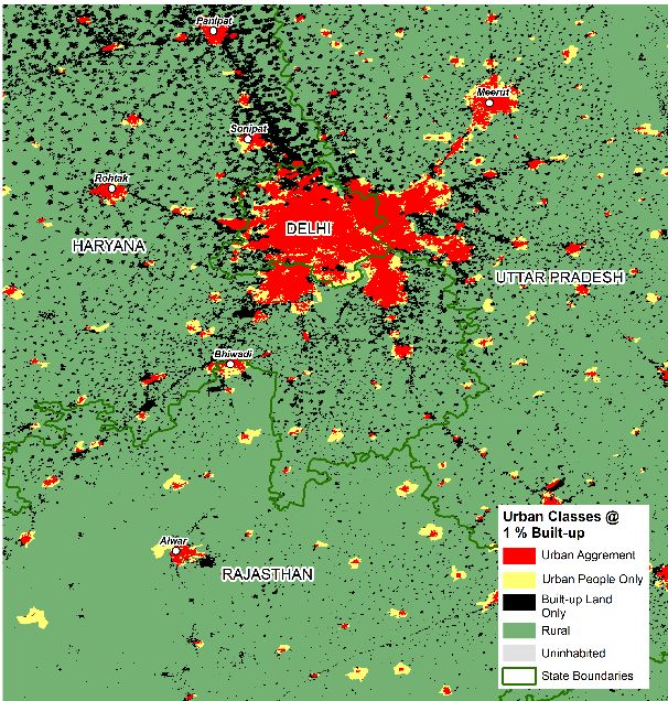
Data 2019, 4, 35                                                                                                       8 of 16
                                (a)                                                      (b)

                                (c)                                                      (d)
      Figure 2. Close-ups of Delhi and surrounding state, 2011: clockwise, the panels indicate (a) population
           Figure 2. Close-ups of Delhi and surrounding state, 2011: clockwise, the panels indicate (a) population
      density, (b) Census
           density,        Classes,
                    (b) Census Classes,  Census
                                     (c)(c) Census++GHSL
                                                    GHSL class at50%
                                                         class at 50%built-up
                                                                       built-up  threshold,
                                                                              threshold, (d) (d) Census
                                                                                             Census       + GHSL
                                                                                                      + GHSL class class
      at 1%atbuilt-up  threshold.
              1% built-up threshold.

3. Methods
    3. Methods
     In constructing   grids
          In constructing    of population
                          grids of populationand
                                               andurban
                                                    urbanareas,
                                                          areas, we
                                                                 we applied
                                                                    applied aa set
                                                                                setofofcommon
                                                                                        commonprinciples
                                                                                               principlesto to all
data all
     production;   and for the
         data production;   andurban   classification
                                  for the             grids, some
                                           urban classification    additional
                                                                 grids,         methodological
                                                                        some additional          considerations
                                                                                           methodological
wereconsiderations
      taken into account.   Theinto
                    were taken   issues  are discussed
                                     account. The issuesin turn.
                                                         are discussed in turn.

     3.1. Matching
3.1. Matching      Spatial
               Spatial     Units
                       Units     withCensus
                              with    CensusTabulations
                                             Tabulations
         As mentioned
     As mentioned      in in Section2.1.2,
                           Section    2.1.2,modifications
                                            modifications to
                                                           tosome
                                                              somespatial
                                                                     spatialboundaries
                                                                              boundaries werewere
                                                                                               necessary to
                                                                                                   necessary to
    properly  link the  detailed PCA   census tabulations with the correct spatial units. (As some  readers
properly link the detailed PCA census tabulations with the correct spatial units. (As some readers may
    may be aware, the input data from ML Infomap includes population attributes. We did not use those
be aware, the input data from ML Infomap includes population attributes. We did not use those census
    census data in this research, but rather, after validating census codes and adding missing units,
data in this research, but rather, after validating census codes and adding missing units, particularly
    particularly for those classified as “outgrowths”, we re-matched the PCA records to the spatial
for those classified as “outgrowths”, we re-matched the PCA records to the spatial boundaries as
described here.) The match of PCAs to the spatial data was made on the following identifiers common
to the two databases: (1) state, district, subdistrict (e.g., tehsil), and settlement codes, (2) ward codes
where applicable, and (3) outgrowth identifiers. In cases of conflicting information between the PCAs
and the spatial information, we gave precedence to the information supplied in the PCAs but checked
each potentially problematic match.
     One complication in the ML Infomap spatial boundary data is that outgrowths are listed under
their rural village identifier codes only. Fortunately, the PCA data on outgrowths include both the
urban ward codes and rural village codes, thus enabling a match with the spatial records. A further
complication is that in 207 cases, an outgrowth was split between a rural village component and a
second component that (although also legally rural) was the part designated as an outgrowth of an
adjacent statutory town. Case-by-case inspection showed that a combination of PCA and spatial-data
variables could identify each of the two parts of such outgrowths. The PCA records report population
and other census information separately for the two components of the divided outgrowths, so there
would appear to be no risk of double-counting population and other PCA attributes.

3.2. On the Use of Thiessen Polygons
     Generally, spatial data on settlement boundaries are available in polygon form. However, some
more remote or less populous states have regions in which settlements are represented by points
instead of polygons. To create spatially contiguous data that can be gridded, for the point-format
would appear to be no risk of double-counting population and other PCA attributes.
3.2. On the Use of Thiessen Polygons
Generally, spatial data on settlement boundaries are available in polygon form. However, some
Data 2019, 4, 35 9 of 16
more remote or less populous states have regions in which settlements are represented by points
instead of polygons. To create spatially contiguous data that can be gridded, for the point-format
settlements we applied a geoprocessing tool in ArcGIS to create Thiessen polygons. These polygons
are defined
definedasasthethe area
area thatthat is closest
is closest topoint
to each eachrelative
point relative to points,
to all other all other
andpoints,
serve asand serve as
hypothetical
hypothetical boundaries in the absence
boundaries in the absence of official units. of official units.
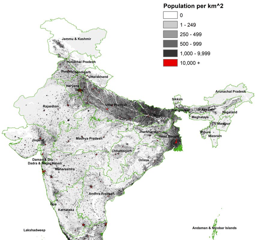
Figure 3 illustrates the transformation
transformation from points to Thiessen polygons. For For aa region in which
points represent settlements,
settlements, the the area of the un-subdivided
un-subdivided regionregion was allocated
allocated according
according to the
placement
placement of the points, producing fictive boundaries boundaries around each each point.
point. For
For states
states with
with both
polygons
polygons and points, the Thiessen polygons were always bounded by the surrounding sub-district
level boundaries.
boundaries. In areas
areas where
wheremany manypoints
pointswere
wereprovided,
provided,we weexpected
expecteda relatively
a relatively small
small margin
margin of
of error.
error. However,
However, forfor sparse
sparse andand typically
typically more
more mountainous
mountainous areas,
areas, somesome large
large areas
areas hadhad relatively
relatively few
few settlement
settlement pointspoints
withinwithin
them, them,
which which
producedproduced less representations
less realistic realistic representations of boundaries.
of boundaries. Examples
Examples of both types of area are
of both types of area are shown in Figure 3. shown in Figure 3.
Figure 3. Transformation of point data to Thiessen polygons.
3.3. Transforming VectorFigure 3. Transformation
Polygons to Raster Gridsof point data to Thiessen polygons.
Because vector
3.3. Transforming polygons
Vector Polygonsaretoirregularly
Raster Gridsshaped, to transform vector data to a uniform grid we
used a proportional allocation rule [26] to deal with contributions from multiple areal units to a single
grid cell, or from a single areal unit to multiple grid cells. This method is widely used in other gridded
population data products [27]. We followed standard practice in removing waterbodies and areas
of permanent ice before creating grids of population distribution and urban areas [27]. (The original
spatial data from ML Infomap also delineated water bodies in some but not all states, or in some but
not all areas within a state. For example, no water is depicted in or around Kolkata, a deltaic city
that is located near several major rivers and their tributaries. Due to these inconsistencies, we used a
different, more systematic water mask.) The 30 m GHSL data layer indicates major areas of surface
water and permanent ice. After simplifying the detailed spatial information in these data (see Figure 4),
we used these spatial data as a water mask. The vast majority (about 90%) of the water bodies that
were indicated in the ML Infomap data were also detected by GHSL (even if not all water bodies were
correctly identified as water by the GHSL). Because water bodies identified in the original ML Infomap
spatial data are uninhabited, any waterbody polygon that was not masked by GHSL remains in our
collection as an uninhabited polygon.
Data 2019, 4, 35 10 of 16
Data 2018, 3, x FOR PEER REVIEW 10 of 17
Figure 4. Original
Figure andand
4. Original simplified data
simplified dataused
usedas
as aa mask toindicate
mask to indicatewater
water (and
(and permanent
permanent ice) areas.
ice) areas.
DataData
that were originally
that were not not
originally in supplied in Geographic
in supplied in Geographic World
World Geodetic
GeodeticSystem
System(WGS)
(WGS)1984 1984 were
transformed from their
were transformed original
from map projection
their original and all
map projection gridding
and waswas
all gridding undertaken
undertaken in in
Geographic
GeographicWGS
1984. WGS
Even1984. Eventhe
though though theunits
raster rasterwere
unitsregular
were regular quadrilateral
quadrilateral grids,
grids, duedue
totothe
theEarth’s
Earth’s curvature
curvature the
the land area of a 30” (nominally, 1 km) grid cell at the southern tip of
land area of a 30” (nominally, 1 km) grid cell at the southern tip of India is greater India is greater than it is it
than at is
theat the
northern tip. For this reason, it is necessary to construct a measure of population density
northern tip. For this reason, it is necessary to construct a measure of population density rather than rather than
population counts. For this, area grids are necessary. Two area grids accompany this data collection:
population counts. For this, area grids are necessary. Two area grids accompany this data collection:
A land area grid which indicates the total land area in each grid cell. (As noted above, water
• A land areaare
bodies grid which indicates the total land area in each grid cell. (As noted above, water
removed).
bodies
are removed).
A land area grid that indicates the land area of a grid cell in a given Indian state. This allows for
• A land
thearea
landgrid
area that indicates
of border zonesthe
(as land area
well as of a grid
in coastal celltoinbea treated
areas) given Indian state. This allows for
fractionally.
the land area of border zones (as well as in coastal areas) to be treated fractionally.
In Figure S1, a flow diagram depicts the processes used to transform vector to raster data from
census data alone. Note the two variants used to construct the population grids and urban
In Figure S1, a flow diagram depicts the processes used to transform vector to raster data from
classification Census Classes grids. The processes used to generate the urban Census + GHSL grids is
census data alone. Note the two variants used to construct the population grids and urban classification
laid out in Balk et al. [18] with the modification that the census units are from the Indian census rather
Census Classes grids. The processes used to generate the urban Census + GHSL grids is laid out in
Balk et al. [18] with the modification that the census units are from the Indian census rather than the
US census. Additional details for the urban grids are described below. The resulting population grid is
shown inDataFigure
2018, 3, x5.
FOR PEER REVIEW 11 of 17
Figure 5.5.Population
Figure density,India
Population density, India 2011.
2011.
3.4. Construction of Urban Classes
We constructed two urban classification grids, one based exclusively on census information and
the other produced by integrating the census classifications with GHSL data.Data 2019, 4, 35 11 of 16
3.4. Construction of Urban Classes
We constructed two urban classification grids, one based exclusively on census information and
the other produced by integrating the census classifications with GHSL data.
3.4.1. Census-Only Grids
The first classification grid, which we denoted as Census Class, is based only on the official census
categorization of settlements. As discussed earlier, these categories include statutory towns (STs),
outgrowths (OGs), census towns (CTs), and rural villages. Wards which are part of a statutory town
for which we had ward-level spatial data, are indicated as components of a statutory town. The census
classification was transformed from polygon to grid format using a majority rule: the classification
indicated in the grid cell is the majority class of the input vector polygons. For example, a cell
comprised of 51% of ST units (by area) and 49% of CT units would be classified as ST. If multiple
settlement classes overlay a cell—usually something that occurs on the outskirts of urban areas—the
maximum contributor was assigned the classification even if the value was less than the majority of
Data 2018,
the 3, x area.
cell’s FOR PEER
TheREVIEW
resulting grid for all India is shown in Figure 6. 12 of 17
Figure
Figure 6. Urban
6. Urban classifications
classifications based
based on on census
census classes,
classes, India
India 2011.
2011.
A summary of the Census Class grid is presented in Table 3. Corresponding to the census’s national
A summary of the Census Class grid is presented in Table 3. Corresponding to the census’s
urban estimates, 31% of India’s population lives in one of the three urban settlement types. Twenty-six
national urban estimates, 31% of India’s population lives in one of the three urban settlement types.
percent of the population lives in areas classified as statutory towns, which make up 2.5% of India’s
Twenty-six percent of the population lives in areas classified as statutory towns, which make up 2.5%
land area. Census towns and outgrowths occupy far less area, and are home to much less of India’s
of India’s land area. Census towns and outgrowths occupy far less area, and are home to much less
urban population, but outgrowths (which occupy less than 0.1% of all land area) are home to more
of India’s urban population, but outgrowths (which occupy less than 0.1% of all land area) are home
than 4 million persons. Average population densities for these three classes indicate a continuum of
to more than 4 million persons. Average population densities for these three classes indicate a
urban locations: notably, outgrowths have population densities above 1200 persons/km2 , more than
continuum of urban locations: notably, outgrowths have population densities above 1200
four times the average for villages.
persons/km2, more than four times the average for villages.
To demonstrate the utility of these spatial data, and to anticipate results from our combined
census–GHSL grid, Table 3 also shows the GHSL built-up percentage of each type of urban area. To
estimate these built-up percentages, we overlay the census data layer with the GHSL built-up raster
and compute the average value for each census class. As with population density, a clear gradient is
seen across the classes. We find that although outgrowths are legally rural, they exhibit built-up
densities characteristic of statutory towns and census towns.Data 2019, 4, 35 12 of 16
To demonstrate the utility of these spatial data, and to anticipate results from our combined
census–GHSL grid, Table 3 also shows the GHSL built-up percentage of each type of urban area.
To estimate these built-up percentages, we overlay the census data layer with the GHSL built-up raster
and compute the average value for each census class. As with population density, a clear gradient
is seen across the classes. We find that although outgrowths are legally rural, they exhibit built-up
densities characteristic of statutory towns and census towns.
Table 3. Population, area, and population density (2011), and estimates of percentage built-up (2014),
by official census classifications, India.
Census Population Area Population Built-Up
Classification Count % km2 % Density %
Statutory Town 318,562,520 26.3% 80,109 2.5% 3977 14.4
Census Town 54,280,980 4.5% 26,234 0.8% 2069 10.2
Outgrowth 4,264,979 0.4% 3436 0.1% 1241 8.7
Village 833,746,498 68.9% 2,850,979 87.2% 292 0.6
Uninhabited 0 0.0% 307,377 9.4% - 0.1
NB: These summaries were produced from the underlying vector data. Statistics based on the gridded products will
differ slightly due to rounding and the majority-rule assignment of each class to a given grid cell.
3.4.2. Census and GHSL-Based Classification
The second classification grid integrates the official census classifications with the GHSL built-up
layer, producing an urban/rural schema that we have described in detail elsewhere [18]. The general
idea is to create a two-way classification of land, with one dimension reflecting the official urban and
rural definitions and the other summarizing the built-up area estimate from GHSL. For the official
classifications, we treat a location as urban if it is classified as an ST, CT or OG, and otherwise take it
to be rural or uninhabited, if designated as such in the boundary data (see Table 1). For the built-up
land layer, we similarly adopt a binary measure based on thresholds of built-up proportions in each
raster cell, classifying each cell as either built-up or not built-up according to its density relative to the
chosen threshold. Two thresholds were considered here: a 50% built-up threshold, which is the most
commonly-cited threshold for defining urban land from GHSL [21] and a 1% threshold, for greater
inclusivity [19].
This combination yields four classes: (1) a class of urban agreement (denoted as UAg), in which
an area is officially classified as urban and also exceeds the GHSL density threshold; (2) a class of
area we denote as urban people only (UPO) for areas that are officially urban but which fall short of
the GHSL threshold; (3) a class of built-up land only (BULO) for areas that are not officially urban but
which nevertheless exceed the density threshold; (4) a rural extent class (RE) for land that is neither
officially urban nor sufficiently built-up; and (5) because the boundary data identified uninhabited areas,
we constructed a separate class for that as well. We integrated the resulting four classes of UAg, UPO,
BULO, and RE (along with uninhabited) to produce a single grid.
To carry out this process, the high-resolution (250 m) GHSL data were vectorized and overlaid
with the census vector data. The final product remains in vector format and can be rendered to a raster
grid at the same 250 m resolution (users may coarsen it to 1 km to match the other grids, and in all
cases will have to decide how to treat mixed-class cells when rasterizing.) The results are presented in
Figure 7.Data 2019, 4, 35 13 of 16
Data 2018, 3, x FOR PEER REVIEW 14 of 17
Figure7.7.Urban
Figure Urbanclassifications
classificationsbased
basedon
oncensus
censusclasses
classescombined with
combined GHSL
with 50%
GHSL built-up,
50% India
built-up, 2011.
India
2011.
A summary of these classes (using both the 50% and 1% built-up thresholds), which shows the
population, land area, and the average built-up fraction, is given in Table 4. As the table shows, areas
A summary of these classes (using both the 50% and 1% built-up thresholds), which shows the
that are both officially urban and sufficiently built-up, that is, areas of urban agreement (UAg), are home
population, land area, and the average built-up fraction, is given in Table 4. As the table shows, areas
to 10.8 percent of India’s population but account for only 0.4% of its land area. These urban-agreement
that are both officially urban and sufficiently built-up, that is, areas of urban agreement (UAg), are
areas, which might be regarded as core-urban locations, are more than 75% built-up, a level well above
home to 10.8 percent of India’s population but account for only 0.4% of its land area. These urban-
the 50% definitional threshold. Their average population density exceeds 10,000 persons/km2 , more
agreement areas, which might be regarded as core-urban locations, are more than 75% built-up, a
than 2.5 times the statutory town average population density. In contrast, about 1 in 5 persons in India
level well above the 50% definitional threshold. Their average population density exceeds 10,000
lives in an area that is officially urban but which is less than 50% built-up; yet such UPOs areas occupy
persons/km2, more than 2.5 times the statutory town average population density. In contrast, about
much more land than do the areas of urban agreement. By definition, UPO areas fall short of the 50%
1 in 5 persons in India lives in an area that is officially urban but which is less than 50% built-up; yet
GHSL threshold, but the degree to which they do is striking: they are less than 5% built-up on average.
such UPOs areas occupy much more land than do the areas of urban agreement. By definition, UPO
Nevertheless, these areas have high population densities, more than 2500 persons/km2 . Finally, areas
areas fall short of the 50% GHSL threshold, but the degree to which they do is striking: they are less
that are built-up but not officially classified as urban (BULO) are home to only 5.5 million residents
than 5% built-up on average. Nevertheless, these areas have high population densities, more than
across India. Although not as dense as UAg or UPO areas, the population densities in these areas
2500 persons/km2. Finally,2 areas that are built-up but not officially classified as urban (BULO) are
exceed 1000 persons/km . The presence of BULO areas varies considerably across states, supporting
home to only 5.5 million residents across India. Although not as dense as UAg or UPO areas, the
recent research findings that indicate considerable state-specific variation in urbanization (perhaps due
population densities in these areas exceed 1000 persons/km2. The presence of BULO areas varies
to state-specific incentives or development initiatives); in some states, urbanization is both widespread
considerably across states, supporting recent research findings that indicate considerable state-
and decentralized, occurring outside major cities [25].
specific variation in urbanization (perhaps due to state-specific incentives or development
Table 4 and Figures 2 and 5, and Figure S2 reveal that these classifications are sensitive to the
initiatives); in some states, urbanization is both widespread and decentralized, occurring outside
built-up threshold.
major cities [25].
Table 4 and Figures 2, 5, and S2 reveal that these classifications are sensitive to the built-up
threshold.Data 2019, 4, 35 14 of 16
Table 4. Population, area, and population density (2011), and estimates of percentage built-up (2014),
according to urban classification based on Census + GHSL (satellite-derived) built-up area data, India.
Population Area Population Built-Up
Threshold Urban Classification
Count % km2 % Density %
Urban Agreement (UAg) 130,203,192 10.8% 12,569 0.4% 10,359 78.3
Urban People Only (UPO) 246,902,934 20.4% 96,238 3.0% 2566 4.7
50 Built-Up Land Only (BULO) 5,554,092 0.5% 5061 0.2% 1097 66.8
Rural Extent (RE) 828,194,760 68.4% 2,830,261 87.5% 293 0.4
Uninhabited - 290,373 9.0% 0.1
Urban Agreement (UAg) 241,523,146 19.9% 40,706 1.3% 5933 35.3
Urban People Only (UPO) 135,582,980 11.2% 68,101 2.1% 1991 0.0
1 Built-Up Land Only (BULO) 86,191,197 7.1% 140,894 4.4% 612 11.3
Rural Extent (RE) 747,557,654 61.7% 2,697,763 83.4% 277 0.0
Uninhabited - 287,038 8.9% 0.0
As Tables 3 and 4, and Figures 6 and 7 show, the two different urban classes reveal different aspects
of urbanization. The availability of both official and remotely-sensed measures will enable a wide
community of users to examine India’s complex patterns of urbanization in fine-grained spatial detail.
4. User Notes
These data were constructed to nest into many of the more commonly used global gridded data
products at a 1-km resolution (such as the Gridded Population of the World (GPW) version 4 [28]). The
data also nest directly into existing gridded projections of future population under scenarios such as the
Shared Socioeconomic Pathways (SSPs) [29] when aggregated to 7.50 resolution [30]. In the case of the
latter, the improvements over existing Indian spatial population data offered by this product, as well
as the new, spatially explicit information contained in urban classification grids, may improve the
ability of the research community to produce scenario-based projections of population/urbanization
outcomes for India, a country of substantial importance in the global-change community.
Supplementary Materials: The following are available online at http://www.mdpi.com/2306-5729/4/1/35/s1.
Figure S1: Process for Population Grid and Urban Census Class Grid, Figure S2.: Urban Classifications based on
Census Classes combined with GHSL 1% Built-Up, India 2011.
Author Contributions: Conceptualization, D.B. and M.R.M.; methodology, D.B., M.R.M. and H.E.; software and
programming, M.R.M., N.L., H.E., E.M. and B.J.; validation, N.L. and B.J.; formal analysis, D.B. and M.R.M.; data
curation, D.B., M.R.M., N.L., H.E. and E.M.; writing—original draft preparation, D.B. and M.R.M.; writing—review
and editing, D.B., M.R.M., B.J. and E.M.; visualization, D.B. and E.M.; supervision, project administration, and
funding acquisition, D.B., M.R.M. and B.J.
Funding: This work was funded in large part by the US National Science Foundation award #1416860 to the City
University of New York, the Population Council, the National Center for Atmospheric Research (NCAR), and the
University of Colorado at Boulder, with additional support from the Andrew Carnegie Fellowship (G-F-16-53680)
from the Carnegie Corporation of New York to Deborah Balk and the European Commission Contract number
2018.CE.16.BAT.050 to Bryan Jones, Deborah Balk, and Mark Montgomery.
Acknowledgments: ML Infomap data were obtained from the Princeton University Library and the Baruch
College Library, when Balk was affiliated with both institutions. We are indebted to T. Wangyal Shawa and
Frank Donnelly, two invaluable and resourceful spatial librarians at Princeton University and Baruch College,
respectively. We thank Khizra Ahmed and Anastasia Clark for research assistance with data acquisition, curation
and documentation, and programming support.
Conflicts of Interest: The authors declare no conflict of interest.
References
1. Census of India. Available online: http://www.censusindia.gov.in/DigitalLibrary/MFTableSeries.aspx
(accessed on 4 December 2018).
2. Bhagat, R.B.; Mohanty, S. Emerging Pattern of Urbanization and the Contribution of Migration in Urban
Growth in India. Asian Popul. Stud. 2009, 5, 1744–1749. [CrossRef]Data 2019, 4, 35 15 of 16
3. Denis, E.; Marius-Gnanou, K. Toward a Better Appraisal of Urbanization in India. Cybergeo Eur. J. Geogr.
2011, 59. [CrossRef]
4. Deuskar, C.; Stewart, B. Measuring Global Urbanization using a Standard Definition of Urban Areas: Analysis
of Preliminary Results. In Proceedings of the Land and Poverty Conference 2016: Scaling up Responsible
Land Governance, Washington, DC, USA, 14–18 September 2016.
5. Balk, D.; Pozzi, F.; Yetman, G.; Deichmann, U.; Nelson, A. The distribution of people and the dimension of
place: Methodologies to improve the global estimation of urban extents. In Proceedings of the International
Society for Photogrammetry and Remote Sensing, Urban Remote Sensing Conference, Tempe, AZ, USA,
14–16 March 2005.
6. Pesaresi, M.; Huadong, G.; Blaes, X.; Ehrlich, D.; Ferri, S.; Gueguen, L.; Halkia, M.; Kauffmann, M.; Kemper, T.;
Lu, L.; et al. A global human settlement layer from optical HR/VHR RS data: Concept and first results.
IEEE J. Sel. Top. Appl. Earth Obs. Remote Sens. 2013, 6, 2102–2131. [CrossRef]
7. IPCC. Climate Change 2014: Impacts, Adaptation, and Vulnerability. Part A: Global and Sectoral Aspects.
Contribution of Working Group II to the Fifth Assessment Report of the Intergovernmental Panel on Climate Change;
Field, C.B., Barros, V.R., Dokken, D.J., Mastrandrea, M.D., Bilir, T.E., Chatterjee, M., Ebi, K.L., Estrada, Y.O.,
Genova, R.C., et al., Eds.; Cambridge University Press: Cambridge, UK, 2014.
8. IPCC. Climate Change 2014: Impacts, Adaptation, and Vulnerability. Part B: Regional Aspects. Contribution of Working
Group II to the Fifth Assessment Report of the Intergovernmental Panel on Climate Change; Barros, V.R., Field, C.B.,
Dokken, D.J., Mastrandrea, M.D., Bilir, T.E., Chatterjee, M., Ebi, K.L., Estrada, Y.O., Genova, R.C., et al., Eds.;
Cambridge University Press: Cambridge, UK, 2014.
9. Jha, A.K.; Bloch, R.; Lamond, J. Cities and Flooding: A Guide to Integrated Urban Flood Risk Management for the
21st Century; The World Bank: Washington, DC, USA, 2012.
10. World Bank. World Bank’s India Disaster Risk Management Program; Working Paper 102550: Washington, DC,
USA, 2016.
11. Revi, A.; Satterthwaite, D.E.; Aragón-Durand, F.; Corfee-Morlot, J.; Kiunsi, R.B.R.; Pelling, M.; Roberts, D.C.;
Solecki, W. Urban areas. In Climate Change 2014: Impacts, Adaptation, and Vulnerability. Part A: Global and
Sectoral Aspects. Contribution of Working Group II to the Fifth Assessment Report of the Intergovernmental Panel on
Climate Change; Field, C.B., Barros, V.R., Dokken, D.J., Mastrandrea, M.D., Bilir, T.E., Chatterjee, M., Ebi, K.L.,
Estrada, Y.O., Genova, R.C., et al., Eds.; Cambridge University Press: Cambridge, UK, 2014; Chapter 8;
pp. 535–612. [CrossRef]
12. Kundu, A. India’s Sluggish Urbanization and Its Exclusionary Development. In Urban Growth in Emerging
Economies: Lessons from the BRICS; McGranahan, G., Martine, G., Eds.; Routledge: New York, NY, USA, 2014;
pp. 191–232.
13. Kundu, A.; Saraswati, L.R. Changing Patterns of Migration in India: A Perspective on Urban Exclusion.
In International Handbook of Migration and Population Distribution; White, M.J., Ed.; Springer: Dordrecht,
The Netherlands, 2016; Chapter 15; pp. 311–332.
14. Pradhan, K.C. Unacknowledged Urbanisation: The New Census Towns in India. An Introduction to the
Dynamics of Ordinary Towns. In Subaltern Urbanisation in India; Denis, E., Zerah, M.H., Eds.; Springer:
New Delhi, India, 2017; Chapter 2; pp. 39–66. [CrossRef]
15. Center for International Earth Science Information Network—CIESIN—Columbia University. Gridded
Population of the World, Version 4 (GPWv4): Population Count; NASA Socioeconomic Data and Applications
Center (SEDAC): Palisades, NY, USA, 2016. [CrossRef]
16. District Census Handbooks. Available online: www.censusindia.gov.in/2011census/dchb/DCHB.html
(accessed on 4 December 2018).
17. Census of India 2011: Administrative Atlas, Office of the Registrar General & Census Commissioner, India.
Available online: www.censusindia.gov.in/2011census/maps/atlas/administrative_atlas.html (accessed on
4 December 2018).
18. Corbane, C.; Pesaresi, M.; Politis, P.; Syrris, V.; Florczyk, A.J.; Soille, P.; Maffenini, L.; Burger, A.; Vasilev, V.;
Rodriguez, D.; et al. Big earth data analytics on Sentinel-1 and Landsat imagery in support to global human
settlements mapping. Big Earth Data 2017, 1, 118–144. [CrossRef]
19. Balk, D.; Leyk, S.; Jones, B.; Montgomery, M.; Clark, A. Understanding Urbanization: A study of census and
satellite-derived urban classes in the United States, 1990–2010. PLoS ONE 2018, 13, e0208487. [CrossRef]
[PubMed]You can also read