Determination of the Regularization Parameter to Combine Heterogeneous Observations in Regional Gravity Field Modeling - MDPI
←
→
Page content transcription
If your browser does not render page correctly, please read the page content below
remote sensing
Article
Determination of the Regularization Parameter to
Combine Heterogeneous Observations in Regional
Gravity Field Modeling
Qing Liu 1, * , Michael Schmidt 1 , Roland Pail 2       and Martin Willberg 2
 1    Deutsches Geodätisches Forschungsinstitut der Technischen Universität München (DGFI-TUM), Arcisstr. 21,
      80333 Munich, Germany; mg.schmidt@tum.de
 2    Institute for Astronomical and Physical Geodesy, Technical University of Munich, Arcisstr. 21,
      80333 Munich, Germany; roland.pail@tum.de (R.P.); martin.willberg@tum.de (M.W.)
 *    Correspondence: qingqing.liu@tum.de

 Received: 16 April 2020; Accepted: 17 May 2020; Published: 19 May 2020

 Abstract: Various types of heterogeneous observations can be combined within a parameter
 estimation process using spherical radial basis functions (SRBFs) for regional gravity field refinement.
 In this process, regularization is in most cases inevitable, and choosing an appropriate value
 for the regularization parameter is a crucial issue. This study discusses the drawbacks of two
 frequently used methods for choosing the regularization parameter, which are the L-curve method
 and the variance component estimation (VCE). To overcome their drawbacks, two approaches for the
 regularization parameter determination are proposed, which combine the L-curve method and VCE.
 The first approach, denoted as “VCE-Lc”, starts with the calculation of the relative weights between
 the observation techniques by means of VCE. Based on these weights, the L-curve method is applied
 to determine the regularization parameter. In the second approach, called “Lc-VCE”, the L-curve
 method determines first the regularization parameter, and it is set to be fixed during the calculation
 of the relative weights between the observation techniques from VCE. To evaluate and compare
 the performance of the two proposed methods with the L-curve method and VCE, all these four
 methods are applied in six study cases using four types of simulated observations in Europe, and their
 modeling results are compared with the validation data. The RMS errors (w.r.t the validation data)
 obtained by VCE-Lc and Lc-VCE are smaller than those obtained from the L-curve method and
 VCE in all the six cases. VCE-Lc performs the best among these four tested methods, no matter
 if using SRBFs with smoothing or non-smoothing features. These results prove the benefits of the
 two proposed methods for regularization parameter determination when different data sets are to
 be combined.

 Keywords: regional gravity field modeling; spherical radial basis functions; combination of
 heterogeneous observations; regularization parameter; VCE; the L-curve method

1. Introduction
     Gravity field modeling is a major topic in geodesy, and it supports many applications, including
physical height system realization, orbit determination, and solid earth geophysics. To model the
gravity field, approaches need to be set up to represent the input data as well as possible. The global
gravity field is usually described by spherical harmonics (SH), due to the fact that they fulfill the
Laplacian differential equation and are orthogonal basis functions on a sphere; see, e.g., [1,2] for more
detailed explanations. However, the computation of the corresponding spherical harmonic coefficients
requires a global homogeneous coverage of input data. As this requirement cannot be fulfilled,

Remote Sens. 2020, 12, 1617; doi:10.3390/rs12101617                       www.mdpi.com/journal/remotesensing
Remote Sens. 2020, 12, 1617                                                                          2 of 25

SHs cannot represent data of heterogeneous density and quality in a proper way [3,4]. Regional gravity
refinement is, thus, performed for combining different observation types such as airborne, shipborne,
or terrestrial measurements, which are only available in specific regions. Different regional gravity
modeling methods have been developed during the last decades, e.g., the statistical method of Least
Squares Collocation (LSC) [5–7], the method of mascons (mass concentrations) [8–10], and the Slepian
functions [11,12]. The method based on SRBFs will be the focus of this work.
      The fundamentals of SRBFs can be found among others in [13–15]. SRBFs are kernel functions
given on a sphere which only depend on the spherical distance between two points on this sphere [16].
They are a good compromise between ideal frequency localization (SHs) and ideal spatial localization
(Dirac delta functions) [17,18]. Due to the fact that SRBFs are isotropic and characterized by
their localizing feature, they can be used for regional approaches to consider the heterogeneity of
data sources; examples are given by [4,19,20]. Li et al. [21] listed the advantages of using SRBFs in
regional gravity field modeling: they can be directly established at the observation points without
gridding, and they are computationally easy to implement. There are four major factors in SRBF
modeling that influence the accuracy of the regional gravity model [22,23]: (1) the shape, (2) the
bandwidth, (3) the location of the SRBFs, and (4) the extension of the data zone for reducing the
edge effects. Tenzer and Klees [24] compared the performance of different types of SRBFs using
terrestrial data and concluded that comparable results could be obtained for each tested type of SRBFs.
Naeimi et al. [23] showed that SRBFs with smoothing features (e.g., the cubic polynomial function) or
without (the Shannon function) deliver different modeling results. Bentel et al. [25] studied the location
of the SRBFs, which depends on the point grids; the results showed that the differences between SRBFs
types are much more significant than the differences between different point grids. Another detailed
investigation about the location of SRBFs can be found in [26], where the bandwidth of the SRBFs was
also studied, and methods for choosing a proper bandwidth were introduced. Lieb [27] discussed the
edge effects and provided a way to choose area margins in order to minimize edge effects.
      After setting up the aforementioned four factors, heterogeneous data sets can be combined within
a parameter estimation process. Regional gravity modeling is usually an ill-posed problem due
to (1) the number of unknowns related to the basis functions, i.e., here the SRBFs; (2) data gaps;
and (3) the downward continuation. Thus, regularization is in most cases inevitable in the parameter
estimation process. Bouman 1998 [28] discussed and compared different regularization methods,
including Tikhonov regularization [29], truncated singular value decomposition [30], and iteration
methods [31]. We apply the Tikhonov regularization in this study, which can be interpreted as an
estimation including prior information [32]. Instead of minimizing only the residual norm, the norm
of the estimated coefficients is minimized in this procedure. Moreover, it is realized by introducing an
additional condition (also called penalty term) containing the regularization parameter. Choosing an
appropriate value for the regularization parameter is, however, a crucial issue.
      Different methods have been developed for estimating the regularization parameter in the
last decades, such as the L-curve criterion [33,34], the variance component estimation (VCE) [32,35,36],
the generalized cross-validation (GCV) [37–41], and Akaike’s Bayesian information criterion [42–46].
Recently, some new methods have been proposed [47–50], and a summary of existing methods
can be found in [28,51–53]. As two of the most commonly used methods for determining the
regularization parameter, the L-curve method and VCE have been applied in numerous studies for
different research fields. Ramillien et al. [54] applied the L-curve method for the inversion of surface
water mass anomalies; Xu et al. [53] used the L-curve method for solving atmospheric inverse problems;
Xu et al. [55] applied VCE for the geodetic-geophysical joint inversion; and Kusche [56], Bucha et al. [57],
and Wu et al. [58] used VCE in global and regional gravity field modeling; similar applications can be
found in the references therein.
      The L-curve method is a graphical procedure. The plot of the solution norm versus the
residual norm displays an “L-shape” with a corner point, which corresponds to the desired
regularization parameter. Koch and Kusche [32] demonstrated that the relative weighting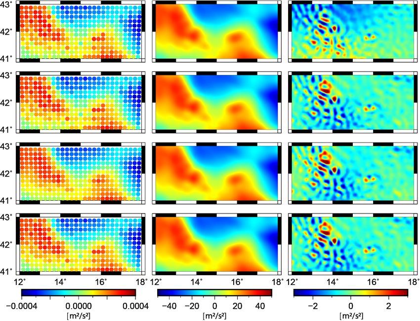
Remote Sens. 2020, 12, 1617                                                                                3 of 25

between different observation types, as well as the regularization parameter, could be determined
simultaneously by VCE. The prior information is added and regarded as an additional
observation technique, and thus the regularization parameter can be interpreted as an additional
variance component. However, in this case, the prior information is required to be of random
character [32]. In most of the regional gravity modeling studies, a background model serves as
prior information. In this case, the prior information has no random character, and the regularization
parameter generated by VCE is not reliable [59]. Lieb [27] presented a case that shows the instability
of VCE. Naeimi [60] showed that VCE delivers larger geoid RMS errors than the L-curve method,
based on GRACE and GOCE data.
     As VCE does not guarantee a reliable regularization solution, and the L-curve method (or other
conventional regularization methods) cannot weight heterogeneous observations [61], the purpose
of this paper is to combine VCE and the L-curve method to improve the stability and reliability
of the gravity solutions. The idea of combining VCE for weighting different data sets only, and a
method for determining the regularization parameter was introduced in the Section “future work” of
both works in [59,60], but have not yet been applied in any further publications. The study in this
manuscript is also inspired by the authors of [62,63]; the formal combines VCE for VLBI intra-technique
combination and GCV for regularization; the latter combines a U-curve method for determining the
regularization parameter and discriminant function minimization (DFM) for estimating the relative
weighting between GPS and InSAR data. Our novel contribution focus on applying this idea for
combining heterogeneous observations in regional gravity field modeling. Thus, we introduce and
discuss in this paper two methods that combine VCE for determining the relative weighting between
different observation types and the L-curve method for determining the regularization parameter,
denoted as “VCE-Lc” and “Lc-VCE”, depending on the order of the applied procedures. Numerical
experiments are carried out to compare their performance to the original L-curve method and VCE.
     This work is organized as follows. Section 2 presents the fundamental concepts of SRBFs, different
types of gravitational functionals, and their adapted basis functions. The parameter estimation,
the Gauss–Markov model as well as the combination model are also introduced. Section 3 is dedicated
to the regularization method, the L-curve method, VCE, and the two proposed combination methods.
In Section 4, the study area, the data used in this study, and the model configuration are explained.
Section 5 discusses the results. The performance of these four regularization methods is compared.
Finally, the summary and conclusions are given in Section 6.

2. Regional Gravity Field Modelling Using SRBF
    In general, a spherical basis function B(x, xk ) related to a point Pk with position vector xk on a
sphere Ω R with radius R and an observation point P with position vector x can be expressed by

                                               ∞                 n +1
                                                   2n + 1       R
                                B(x, xk ) =   ∑ 4π              r
                                                                        Bn Pn (r T r k )                      (1)
                                              n =0

Ref. [4], with x = r · r = r · [cos φ cos λ, cos φ sin λ, sin φ] T , where λ is the spherical longitude, φ is the
spherical latitude, xk = R · r k , Pn is the Legendre polynomial of degree n, and Bn is the Legendre
coefficient which specifies the shape of the SRBF. When Bn = 1 for all n, B( x, xk ) represents the Dirac
delta function, which has ideal spatial localization. With the spherical basis function (1), a harmonic
signal F (x) given on the sphere Ω R or in the exterior space of Ω R , can be described as

                                                         K
                                              F (x) =   ∑ dk B(x, xk ),                                       (2)
                                                        k =1

where K is the number of basis functions. The unknown coefficients dk can be evaluated from
the observations. As will be shown in the following subsection, using these coefficients, any functional
of F (x) can be described.
Remote Sens. 2020, 12, 1617 4 of 25
2.1. Gravity Representations
Various functionals can be derived from the gravitational potential V or from the disturbing
potential T based on field transformations. The corresponding kernels can be derived from the
definition (1) of the basis functions, and are listed in Table 1.
Disturbing potential: The disturbing potential T is defined as the difference between the gravity
potential W and the normal gravity potential U,
T = W − U, (3)
where the latter is the potential related to the level ellipsoid. The gravity potential W consists of
two parts: the gravitational potential V and the centrifugal potential Z, i.e.,
W = V + Z. (4)
Combining Equation (3) and Equation (4) yields [2]
T = V − U + Z. (5)
The disturbing potential T can be represented by
K
T (x) = ∑ dk B(x, xk ). (6)
k =1
Gravitational potential difference: The satellite gravity field mission Gravity Recovery and
Climate Experiment (GRACE) [64] consists of two satellites A and B. The main observable is the exact
separation distance between the two satellites and its rate of change [65]. Several GRACE products
exist (level 0 to level 2) [66,67]; the gravitational potential V can be computed from the level 2 products.
In many studies (see, e.g., [20,27,60,68]), the differences between the gravitational potential values V of
A and B are used as observations ∆V, i.e., ∆V (x A , xB ) = V (x A ) − V (xB ). Including the measurement
error e, the observation equation reads
K
∆V (x A , xB ) + e(x A , xB ) = V (x A ) − V (xB ) + e(x A , xB ) = ∑ d k B (x A , x B , xk ). (7)
k =1
Gravity disturbance: The gravity disturbance is used in airborne and terrestrial gravity
field determination. The gravity disturbance vector δg is expressed as the gradient of the disturbing
potential T
T
∂T ∂T ∂T
δg = , , = gradT. (8)
∂x ∂y ∂z
In spherical approximation, the magnitude of the gravity disturbance can be written as
∂T
δg = − = − Tr , (9)
∂r
its observation equation reads
K
δg(x) + e(x) = ∑ dk Br (x, xk ). (10)
k =1
Gravity gradient: Equipped with a 3-axis gradiometer, the satellite mission Gravity Field
and Steady-State Ocean Circulation Explorer (GOCE) [69] observed the gravity gradients Vab with
a, b ∈ { x, y, z}, i.e., all second-order derivatives of the gravitational potential VRemote Sens. 2020, 12, 1617 5 of 25
Vxx Vxy Vxz
V = Vyx Vyy Vyz (11)
Vzx Vzy Vzz
with Vxy = Vyx , Vxz = Vzx , Vyz = Vzy and trace V = 0 due to the Laplacian differential equation.
∂2 V
The observation data of GOCE used in this study are simulated as the radial component Vrr = ∂r2
,
and the observation equation reads
K
Vrr (x) + e(x) = ∑ dk Brr (x, xk ). (12)
k =1
For each type of gravitational functional, the adapted basis functions are derived by the zeroth,
first, or second order derivatives of Equation (1), and they are listed in Table 1. Basis functions adapted
to other functionals of the disturbing potential which are not used here can be found in [20,27,70].
Table 1. Kernels, i.e., the adapted basis functions for different gravitational functionals.
Gravitational Functionals Adapted Basis Function B(x, xk )
n +1
Disturbing potential B(x, xk ) = ∑∞ 2n+1 R
n=0 4π r Bn Pn (r T r k )
n +1 n +1
B (x A , x B , xk ) = ∑ ∞ 2n+1 R T T
ine Gravitational potential difference n=0 4π Bn { r A Pn (r A r k ) − rRB Pn (r B r k )}
n +1
ine Gravity disturbance Br (x, xk ) = ∑∞ 2n+1 (n+1) R
n=0 4π r r Bn Pn (r T r k )
n +1
ine Gravity gradients Brr (x, xk ) = ∑∞ 2n+1 (n+1)(n+2) R
n=0 4π r2 r Bn Pn (r T r k )
2.2. Types of Spherical Radial Basis Functions
Different types of SRBFs can be found among others in [4,68]; the frequently used types
include the Shannon function, the Blackman function, the cubic polynomial (CuP) function, and the
Poisson function. Two types of band-limited SRBFs are used in this work, one without smoothing
features (Shannon function), i.e., their shape coefficients (Legendre coefficients) equal to 1 for all
frequencies within a certain bandwidth, and the other one with smoothing features (CuP function).
The Shannon function has the simplest representation; its Legendre coefficients are given by
(
1 for n ∈ [0, Nmax ]
Bn = (13)
0 else
In case of the CuP function, the Legendre coefficients are given by a cubic polynomial, namely,
(
n
(1 − Nmax )2 (1 + N2n ) for n ∈ [0, Nmax ]
Bn = max (14)
0 else
Nmax is a certain degree to which the SRBFs are expanded, representing the cut-off degree.
These two functions for Nmax = 255 are plotted in Figure 1, the top sub-plot and the bottom one
visualize the characteristics in the spatial and the spectral domain, respectively. In the spatial domain,
the Shannon function shows the sharper transition but also the stronger oscillations compared to
the CuP function. In the spectral domain, the Shannon function is characterized by its exact band
limitation without any smoothing features. The CuP function, however, has a smoothing decay.
In this study, we apply both the Shannon function and the CuP function in the same experiments to
test the performance of our proposed regularization methods.Remote Sens. 2020, 12, 1617 6 of 25
Figure 1. The different spherical radial basis functions (SRBFs) in the spatial domain (top, ordinate
values are normalized to 1) and the spectral domain (bottom) for Nmax = 255.
2.3. Parameter Estimation
To determine the unknown coefficients dk in Equation (2), parameter estimation [36] is used
in this study. This process allows the combination of different types of observations with varying
resolutions, accuracies and distributions [71].
2.3.1. Gauss–Markov Model
For one single observation F ( x), the observation equation reads
K
F (x) + e (x) = ∑ dk B(x, xk ), (15)
k =1
B(x, xk ) represents the adapted SRBFs as listed in Table 1. Collecting the observations F (x1 ), F (x2 ), . . . ,
F (xn ) in the n × 1 observation vector f , the Gauss–Markov model
f + e = Ad (deterministic part) with D (f ) = σ2 P−1 (stochastic part) (16)
can be set up. In the deterministic part, e = [e(x1 ), e(x2 ), . . . , e(xn )] T is the n × 1 vector of the
observation errors and A = [ B(x, xk )] is the n × K design matrix containing the corresponding
basis functions. In the stochastic part, D (f ) is the n × n covariance matrix of the observation vector f
with σ2 being the unknown variance factor and P being the given positive definite weight matrix.
Due to the three reasons mentioned in the introduction, namely, (1) the number of unknowns
related to the basis functions, (2) data gaps, and (3) the downward continuation, the normal equation
matrix N = AT PA is ill-posed or even singular. For handling this problem, we introduce an additional
linear model
µd + ed = d with D (µd ) = σd2 P−
d
1
(17)
as prior information. µd is the K × 1 expectation vector of the coefficient vector d, ed is the corresponding
error vector, and D (µd ) is the K × K covariance matrix of the prior information with σd2 the unknown
variance factor and Pd the positive definite weight matrix. Combining the two models (16) and (17)
yields the extended linear model
" # " # " # " #! " # " #
f e A f −1 0
2 P 2 0 0
+ = d with D =σ + σd (18)
µd ed I µd 0 0 0 P− d
1Remote Sens. 2020, 12, 1617 7 of 25
Now the least-squares adjustment can be applied and leads to the normal equations
!
1 T 1 b = 1 AT Pf + 1 Pd µ
2
A PA + 2 Pd d d (19)
σ σd σ2 σd2
The variance factors σ2 and σd2 can either be chosen or estimated within a VCE, and the solution reads
b = (AT PA + λPd )−1 (AT Pf + λPd µ )
d (20)
d
b) = σ2 (AT PA + λPd )−1 ,
D (d (21)
wherein λ = σ2 /σd2 can be interpreted as the regularization parameter, see [4,32]. When µd is set to the
zero vector, Equation (20) reduces to the Tikhonov regularization, and the regularization parameter λ
can be determined by the L-curve method.
2.3.2. Combination Model
To combine different types of heterogeneous data sets for regional gravity field modeling,
combination model (CM) needs to be set up (see, e.g., [4,32]). In general, let f l with l = 1, . . . , L
be the observation vector of the l th observation technique, such as f l = [ Fl (x1 ), Fl (x2 ), . . . , Fl (xnl )] T , el
and Al are the corresponding error vector and the design matrix. Note that for different techniques,
the data are observed as different gravitational functionals and thus, the adapted SRBFs as discussed in
the Section 2.1 must be applied accordingly, Al = [ Bl (x, xk )]. For the combination of the L observation
techniques, an extended Gauss–Markov model can be formulated by including the additional linear
model (17) for the prior information
σ12 P1−1
0 0 ... 0
f1 e1 A1 f1 .. .. ..
f e A
2 2 2
f 0
2 σ22 P2−1 . . .
. . .
. + . = . · d with D .. = .. .. .. ..
. . . . . 0 . . .
(22)
. .. ..
f L e L A L f L .
σL2 P− 1
. . . L 0
µd ed I µd
0 0 ... 0 σd2 P−
d
1
Ref. [27], where Pl is the nl × nl positive definite weight matrix of the lth observation technique.
Applying the least-squares method to Equation (22), the extended normal equations read
!
L L
1 T 1 1 1
∑ ( σ2 Al Pl Al ) + σ2 Pd db = ∑ ( σ2 AlT Pl f l ) + σ2 Pd µd . (23)
l =1 l d l =1 l d
The values for the variance factors can either be chosen or estimated by VCE (refer to Section 3.2).
Consequently, the solution of Equation (23) reads
! −1 !
L L
1 1 1 1
d
b= ∑ ( σ2 AlT Pl Al ) + σ2 Pd ∑ ( σ2 AlT Pl f l ) + σ2 Pd µd . (24)
l =1 l d l =1 l d
The covariance matrix of the unknown parameter vectors reads
! −1
L
1 1
D (d
b) = ∑ ( σ2 AlT Pl Al ) + σ2 Pd . (25)
l =1 l d
Equation (24) can be rewritten asRemote Sens. 2020, 12, 1617 8 of 25
! −1 !
L L
d
b= ∑ (ωl AlT Pl Al ) + λPd ∑ ωl AlT Pl f l + λPd µd , (26)
l =1 l =1
such that λ = b σ12 /b
σd2 is the regularization parameter, and the factors ω1 = b σ12 /b
σ12 = 1,
ω2 = b 2 2
σ2 , . . . , ω L = b
σ1 /b 2 2
σL express the relative weights of the observation vector f l with respect
σ1 /b
to f 1 .
3. Determination of the Regularization Parameter
A critical question of regularization is the selection of an appropriate regularization parameter
λ [72]. In the following, the L-curve method and the VCE will be explained in more detail. Finally,
two new proposed methods are presented as combinations of VCE and the L-curve method.
3.1. L-Curve Method
The L-curve is a graphical procedure for regularization [28,33,34,73]. The norm of the regularized
solution kdbλ − µ k is plotted against the norm of the residuals kb
d ek = k Adbλ − f k by changing
the numerical value for the regularization parameter λ. Moreover, the plot shows a typical
L-curve behavior, i.e., it looks like the capital letter “L” (see Figure 2). The corner point in this L-shaped
curve means a compromise of the minimization of the solution norm (which measures the regularity
of the solution) and the residual norm (which quantifies the quality of fit to the given data), and thus
can be interpreted as the “best fit” point that corresponds to the desired regularization parameter.
It should be mentioned that if the L-curve method is to be applied when different types of
observations are combined, the relative weights ωl in Equation (24) need to be chosen. However, as it
is not possible to know the accurate weights, the solution delivered by the L-curve method alone is,
thus, not reliable.
Figure 2. An example of the L-curve function.
3.2. Variance Component Estimation
Variance component estimation not only estimates the relative weighting between each data
set but also determines the regularization parameter simultaneously. The variance components are
estimated by an iterative process [20,32]. It starts from initial values for σl2 , σd2 , and ends in the
convergence point. The estimations readRemote Sens. 2020, 12, 1617 9 of 25
elT Pl b
el
σl2 =
b b
rl
edT Pd bed
(27)
σ2 =
b b
d rd
el and b
where the residual vectors b ed are given as
(
b− f
el = Al d
b l (28)
ed = d − µd
b b
and rl , rd are the partial redundancies, which are the contributions of the observations f l and the
prior information µd to the overall redundancy of Equation (22). The redundancy numbers rl , rd are
computed following Koch and Kusche [32],
rl = nl − trace( 12 AlT Pl Al N −1 )
σl
(29)
rµ = K − trace( 12 Pd N −1 )
σ d
where nl denotes the number of observations in the l th data set, K is the number of coefficients, and
!
L
1 T 1
N = ∑ ( 2 Al P l Al ) + 2 P d . (30)
l =1 σl σd
Starting with initial values for σl2 , σd2 , an initial solution for d
b can be calculated, and it leads to the new
estimations for b 2
σl , b 2
σd in Equation (27). The procedure iterates until the convergence point is reached.
As in the model represented by Equation (17) the prior information is regarded as an additional
type of noisy observation, µd is expected to be of stochastic character. However, when the background
model serves as prior information, µd is a deterministic vector. Consequently, ed = d − µd is
also deterministic, and the requirements for the Equation (17) are in fact not fulfilled. Thus, in this case
the regularization parameter λ generated by VCE is not reliable.
3.3. Combination of VCE and the L-Curve Method
To overcome the drawbacks in the L-curve method and in the VCE for combining heterogenous
observations, two methods are proposed and applied in this study, namely, VCE-Lc and Lc-VCE.
3.3.1. VCE-Lc
Figure 3 illustrates the procedure of the VCE-Lc. In the first step, the VCE is applied to determine
the relative weights between the observation types. This step gives the relative weighting factors ωl ,
and a regularization parameter λVCE simultaneously, after the iteration converges. In the second step,
the weighting factors ωl are kept, but the regularization parameter λVCE is not used. Instead, a new
regularization parameter is regenerated using the L-curve method. The corner point in the plot of the
regularized solution norm kd bλ − µ kP against the the residual norm kb
d d
ek = k Ad
bλ − f kP corresponds
to the new regularization parameter. In this case, the L-curve method is applied based on the variance
σl2 of each observation type generated by VCE. The corner point in Figure 2 corresponds to the
factors b
new regularization parameter λL-curve .
Thus, the final solution is computed using Equation (26) with the weights ωl from VCE and the
new regularization parameter λL-curve from the L-curve criterion.Remote Sens. 2020, 12, 1617 10 of 25
Figure 3. Analysis and synthesis for combining different types of observations based on the VCE-Lc.
3.3.2. Lc-VCE
Figure 4 illustrates the procedure of the Lc-VCE. In contrast to the VCE-Lc, in the Lc-VCE the
L-curve method is applied first based on chosen values for the relative weights ωl in Equation (24).
A regularization parameter λL-curve is obtained in the first step, and it is used for defining the value of
σd2 in the variance component estimation.
In the second step, the VCE is applied with initial values σ12 = σ22 = . . . = σL2 and σd2 = σ12 /λL-curve .
After each iteration within the VCE, the value of σd2 is set to σ12 /λL-curve again, with the new value of
σ12 obtained in this iteration. In this case, the regularization parameter λ calculated from the L-curve
method will be kept, but the relative weighting factors ωl are recomputed in each iteration step.
The final solution is computed using Equation (26) with the relative weights ωl and the regularization
parameter λL-curve .
Figure 4. Analysis and synthesis for combining different types of observations based on the Lc-VCE.Remote Sens. 2020, 12, 1617 11 of 25
It is worth clarifying that the solution obtained from the Lc-VCE is not unique. Due to the fact
that the regularization parameter λL-curve is fixed during VCE, the results change when λL-curve refers
to different observation techniques. To be more specific, as already mentioned in the last paragraph,
the value of σd2 is set to σ12 /λL-curve after each iteration. Thus, the value of σd2 changes by setting
different observation types as σ12 , and the results of Equation (24) change, consequently.
To summarize, the purpose of these two proposed methods is to benefit from the L-curve method
and VCE, and thus to overcome the drawbacks when using each method individually. VCE-Lc fixes the
relative weights of each observation technique first and tries to find a “best fit” regularization parameter,
whereas Lc-VCE fixes the regularization parameter first and then tries to find the relative weights for
each observation technique.
4. Numerical Investigation
4.1. Data Description
The data used in this study are provided by the ICCT (Inter-Commission Committee on Theory)
Joint Study Group (JSG) 0.3 “Comparison of current methodologies in regional gravity field modelling”,
part of the IAG (International Association of Geodesy) programme running from 2011 to 2015.
The observation data are simulated from the Earth Gravitational Model EGM2008 [74] and are
provided along with simulated observation noise. In this study, all observations are simulated
in the sense of disturbing gravity field quantities, i.e., functionals of the disturbing potential T:
disturbing potential differences ∆T for GRACE, the first order radial derivatives Tr for the terrestrial
and airborne observations as well as the second order radial derivatives Trr for GOCE. The standard
deviations of the given white noise are 8 · 10−4 m2 /s2 for GRACE, 10 mE for GOCE, 0.01 mGal for the
terrestrial data and 1 mGal for the airborne data. The study area chosen here is “Europe”, where the
validation data are also simulated from the EGM2008 and provided on geographic grid points in terms
of disturbing potential values T.
Figure 5 illustrates the available observation data as well as the validation data. The two validation
areas are presented with black rectangles: the larger area (Synthesis Data I) has a spatial resolution
of 300 × 300 and is simulated with a maximum degree of 250; the smaller area (Synthesis Data II)
has a spatial resolution of 50 × 50 and with a maximum degree of 2190. Four types of observations
are included:
1. GRACE data: provided along the real satellite orbits of GRACE (green tracks in Figure 5), with a
time span of one month.
2. GOCE data: provided along the real satellite orbits of GOCE (red tracks), covering a full repeat
cycle of 61 days.
3. Terrestrial data: provided in a regular grid on the surface of the topography (DTM2006.0 [75])
with two different resolutions: one over an area of 20◦ × 30◦ (latitude × longitude) with a grid
spacing of 30’ (blue dots) and the other one over an inner area of 6◦ × 10◦ with a grid spacing of
5’ (yellow highlighted area).
4. Airborne data: provided on two different flight tracks: one over the Adriatic Sea (magenta striped
area) and the other one over Corsica connecting Southern Europe with Northern Africa (cyan
striped area).Remote Sens. 2020, 12, 1617 12 of 25
Figure 5. The study area as well as the GRACE, GOCE, terrestrial and airborne observations
This study uses simulated data to take advantage of the availability of validation data. As this is a
conceptual study to compare different methods, it is important to have an accurate validation data
serving as the “true value” so that the gravity modeling result from each method can be evaluated
and compared. Although validation when using real data is also possible, e.g., by comparing to
GNSS/leveling data or to existing regional gravity models in the same region, the accuracy of the
validation data then needs to be assessed beforehand.
4.2. Model Configuration
A Remove–Compute–Restore approach [76,77] is applied in this study, i.e., from each type
of observation, the background model EGM2008 up to spherical harmonic degree 60 is removed and
restored in the synthesis step. The background model serves additionally as prior information, and thus
the vector d of the unknown coefficients contains the gravity information referring to a reference field
(background model) up to degree and order 60. Koch and Kusche [32] pointed out that in this case,
the expectation vector µd can be set to the zero vector [4,27]. We assume that the coefficients have the
same accuracy and are uncorrelated; thus, Pd = I, where I denotes the identity matrix. Further, we set
Pl = I by assuming the measurement errors to be uncorrelated and the same type of observations to
have the same accuracy. These assumptions are commonly used in the existing publications for both
simulated and real data, since it is usually difficult to acquire the realistic full error variance-covariance
matrix, and examples can be found in, e.g., [27,57,58].
As discussed in Section 3.1, the values of σl2 need to be chosen beforehand for the L-curve method.
In studies where different observation types are involved, one might conduct an analysis on the
relative weighting between the data sets in order to apply the L-curve method. Thus, in this study,
empirically chosen values of σl2 are used for each observation type to have a more realistic result for the
L-curve method. Lieb et al. [20] pointed out that the variance factors σl2 depend on the measurement
accuracy, but also on the number, the spectral resolution, and the spatial distribution of the data.
By using only the noise levels of each data set for calculating the variance factors, the σl2 values should
be 0.64 · 10−6 for the GRACE data, 10−22 for the GOCE data, 10−10 for the airborne data, and 10−14
for the terrestrial data. However, Lieb (2017) showed that the airborne and terrestrial data are less
sensitive in the low-frequency part, and their weights could degrade up to six orders of magnitude
when the maximum degree of expansion is low. Taking both factors into consideration, the values
of σl2 are chosen as 10−6 for the GRACE data, 10−22 for the GOCE data, and 10−8 for the terrestrial
data and the airborne data in this study. It is worth mentioning that these values of σl2 are only
approximations, and they are a choice for applying the L-curve method when VCE is not considered.Remote Sens. 2020, 12, 1617 13 of 25
Moreover, the purpose of this study is not to compare between the L-curve method and VCE, but to
compare the two proposed methods with using the L-curve method or VCE individually. The results
for the L-curve method without relative weights (equal weighting between each data set) are also
presented in Section 5.1 as a comparison scenario.
In this study, different observation types are combined in a “one-level” manner, which is also
applied in, e.g., [20,58,68]. The relative weights indicate the contributions of different observation
types [20]. Another way for combining different types of observations is the spectral combination (see,
e.g., in [78–80]), where the (spectral) weights depend on the spectral degree. The spectral weights
at each degree can be incorporated into the (kernel) functions [79], and studies about how to find
the optimal kernels can be found in, e.g., [80,81]. However, details about the spectral combination
technique would go beyond the scope of this study.
Figure 6 presents the computation area ∂ΩC , the observation area ∂ΩO , as well as the investigation
area ∂Ω I . The computation area ∂ΩC should be larger than the observation area ∂ΩO , due to the
oscillations of the SRBFs. The observation area ∂ΩO should be larger than the investigation area ∂Ω I ,
because the unknown coefficients dk cannot be accurately estimated in the border of the observation
area ∂ΩO . Thus, ∂Ω I ⊂ ∂ΩO ⊂ ∂ΩC , and detailed explanations for this extension can be found
in [27,60]. In the analysis step, we estimate the vector db of the unknown coefficients dk related to the
grid points Pk within the computation area ∂ΩC , from the measurements available within the area ∂ΩO .
In the following synthesis step, these coefficients are used for calculating the output gravity functional
within the area ∂Ω I . It has to be mentioned that the points Pk within the computation area ∂ΩC are
defined by a Reuter grid [82]. The Reuter’s algorithm generates a system of homogeneous points on
the sphere [22]. Margins η between the computation area ∂ΩC and the observation area ∂ΩO as well
as between the observation area ∂ΩO and the investigation area ∂Ω I are chosen equally, and they have
to be defined to minimize edge effects in the computation process [20]. In this study, we conducted
the experiments using different margin sizes (from 1◦ to 4◦ ), and the ones (values given in Section 5)
which result in the smallest difference between the estimated disturbing potential and the validation
data are finally chosen.
Figure 6. Extensions for the different areas ∂ΩC of computation, ∂ΩO of observations, and ∂Ω I
of investigation.
The aforementioned four methods for choosing the regularization parameter, i.e., (1) L-curve
method, (2) VCE, (3) VCE-Lc, and (4) Lc-VCE, are applied to six groups of data sets, respectively. The
types of observations involved in the six study cases as well as the corresponding validation data for
each study case are listed in Table 2. These six groups cover the possible combination among the four
data types, to make sure that the comparisons of these four methods are conducted in different data
combination scenario. The computed disturbing potential Tc is compared with the corresponding
validation data Tv and assessed following two criteria:
1. Root mean square error (RMS) of the computed disturbing potential Tc with respect to the
validation data Tv over the investigation area ∂Ω IRemote Sens. 2020, 12, 1617 14 of 25
v
u ∑npoints ( Tv − Tc )2
u
RMS = t (31)
npoints
where npoints is the number of points in the validation data.
2. Correlation coefficient between the estimated coefficients dk collected in the vector d b and the
validation data Tv . It has to be clarified that the estimated coefficients dk and the validation data
Tv are located at different points, and an interpolation is conducted to transit dk to the grid of the
validation data.
The reason that this correlation can be used as a criterion is that the coefficients dk reflect the
energy of the gravity field at their locations. On a sphere embedded in a three-dimensional space,
the energy of a signal F ( x) can be expressed by
Z
E= | F ( x)|2 dΩ R . (32)
ΩR
Combining Equation (2) with Equation (32), it yields
Z K K K Z
E=
ΩR
| ∑ dk B(x, xk )|2 dΩR = ∑ dk ∑ di ΩR
B( x, xk ) B( x, xi )dΩ R . (33)
k =1 k =1 i =1
By inserting the series expansion of the SRBFs (Equation 1) on Ω R to Equation (33) and applying
the addition theorem (details about the equation manipulation can be found in [27]), the energy
contribution Ek (k = 1, 2, . . . , K) at location xk is given as
K Nmax
2n + 1 2
Ek = dk ∑ di ∑ 4π
Bn Pn (riT r k ). (34)
i =1 n =0
When Nmax goes to ∞, and Bn =1 for all n, i.e., in the case of the Dirac delta function, Ek = d2k .
In the case of SRBFs where Nmax 6= ∞, and Bn is not necessarily equal to 1, the relation Ek = d2k
is only approximately valid. However, a higher correlation between the coefficients dk and the
validation data still indicates a better representation of the gravity signal. The same criterion is
used as a quality measure by [23,25].
Table 2. Study cases.
Study Case Data Combination Validation Data
A GRACE + GOCE
B GRACE + Airborne I + Airborne II Synthesis Data I
C GRACE + Terrestrial I
D GOCE + Terrestrial I
ine E Terrestrial II + Airborne I
Synthesis Data II
F GRACE + GOCE + Terrestrial II +Airborne I
5. Results
The experiments are carried out using the Shannon function for both analysis and synthesis.
However, to test the performance of these four methods when a smoothing SRBF is used,
the same experiments are also applied using the CuP function for analysis and synthesis as a
comparison scenario. The maximum degree in the expansion in terms of SRBF is chosen basedRemote Sens. 2020, 12, 1617 15 of 25
on the spatial resolution of the observations [20,57], and it is set to Nmax = 250 for the study cases A
and B; Nmax = 400 for the study cases C and D; Nmax = 2190 for the study cases E; and Nmax = 1050
for the study case F. The margin η between the different areas (Figure 6) is chosen to be 4◦ for the study
cases A, B, C, and D, and 2◦ for the study cases E and F.
For the sake of brevity, only the results of two study cases (case A in Table 3 and case F in Table 4)
are detailed here. Results from the case A and the case F clearly show the drawbacks of VCE and
the L-curve method, respectively. However, results obtained from all study cases, including the RMS
errors and the correlations between the estimated coefficients dk and the validation data Tv of each
method are summarized in the Tables 5 and 6, respectively. The results when using the CuP function
are listed in the Tables 7 and 8.
5.1. Results Using the Shannon Function
5.1.1. Study Case A
GRACE and GOCE observations are combined. Four solutions are estimated according to the
aforementioned four methods for determining the regularization parameter. For each solution, the RMS
error as well as the correlation between the estimated coefficients dk and the validation data Tv are
listed in Table 3. Two scenarios are considered, depending on how the relative weights ωl (or the
variance factors σl2 ) between each observation type are chosen in the L-curve method and Lc-VCE.
In the first scenario, the relative weights ωl are chosen empirically (see Section 4.2). The lowest
RMS error is obtained from the VCE-Lc which is 4.59 m2 /s2 . This method also delivers the highest
correlation between the estimated coefficients dk and the validation data. Lc-VCE gives the second best
RMS value which is 4.61 m2 /s2 (Referring to Section 3.3.2, the solution obtained from Lc-VCE is not
unique, and the results listed here for Lc-VCE are always the best ones, i.e., the solution which gives
the lowest RMS and largest correlation). For each solution, the estimated coefficients dk , the calculated
disturbing potential Tc , as well as its difference to the validation data are plotted in Figure 7. VCE gives
the smallest correlation and the largest difference compared to the validation data. The RMS error
obtained from VCE is 7.84 m2 /s2 , which is ~70% larger than those obtained from VCE-Lc or Lc-VCE.
In reality, it is difficult to choose the empirical weights between different observation
types accurately, as the accuracy of different observation types is not available. As listed in Table 3,
in the second scenario, when no relative weights are applied (equal weighting between data sets),
the performance of the L-curve method decreases, with a 56% increase in RMS error. This increase
demonstrates the importance of accurately weighting different data sets. The result obtained from
the Lc-VCE also decreases slightly, with the RMS error increases from 4.61 m2 /s2 to 5.17 m2 /s2 .
In this scenario, VCE-Lc and Lc-VCE still deliver the lowest and second lowest RMS error, respectively.
The same order applies to the correlation between the estimated coefficients dk and the validation data.
The RMS error from VCE-Lc is 36% and 41% smaller than that delivered by the L-curve method and
VCE, respectively. The RMS error from Lc-VCE is 28% and 34% smaller than that delivered by the
L-curve method and VCE, respectively. VCE still gives the largest RMS error as well as the smallest
correlation, which proves that VCE does not determine the regularization parameter as successful as
the L-curve method, since it gives a worse result than the L-curve method which is based on an equal
weighting between each observation type.Remote Sens. 2020, 12, 1617 16 of 25
Table 3. Results of Study Case A: the root mean square error (RMS) values (unit [m2 /s2 ]) as well as
the correlations for each regularization method, when different relative weights ωl are chosen for the
L-curve method
ωl Chosen Empirically ωl = 1
Regularization Method
RMS Correlation RMS Correlation
L-curve method 4.6185 0.9376 7.2153 0.9078
VCE 7.8374 0.8965 7.8374 0.8965
VCE-Lc 4.5876 0.9384 4.5876 0.9384
Lc-VCE 4.6062 0.9382 5.1655 0.9310
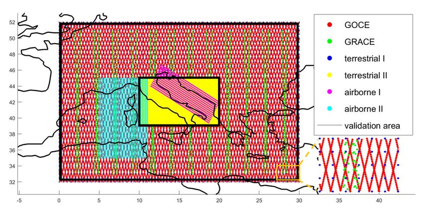
Figure 7. The estimated coefficients dk (left column), the recovered disturbing potential Tc (mid
column), and the differences w.r.t the validation data (right column) for study case A. The results are
obtained using: the L-curve method (first row), VCE (second row), VCE-Lc (third row), and Lc-VCE
(fourth row).
5.1.2. Study Case F
In case F, four data sets (GRACE, GOCE, the terrestrial II, and the airborne I observations)
are combined. Compared to the study case A, the results in the study case F (listed in Table 4)
show a general improvement, in terms of both the two criteria. When the relative weights ωl are
chosen empirically (see Section 4.2), VCE-Lc provides the smallest RMS error 0.84 m2 /s2 , followed byRemote Sens. 2020, 12, 1617 17 of 25
the Lc-VCE. The same order applies to the correlation between the estimated coefficients dk and the
validation data. The L-curve method delivers the largest RMS value with 0.91 m2 /s2 , as well as the
smallest correlation. It shows that the empirically chosen relative weights between different observation
types are not accurate, and it is necessary to estimate the weights with VCE. For each solution,
the estimated coefficients dk , the calculated disturbing potential Tc as well as its difference to the
validation data are plotted in Figure 8. It shows that the L-curve method delivers the largest difference
compared to the validation data.
When no relative weights are applied (equal weighting), the performance of the L-curve
method decreases, with a 61% increase in RMS error. Further, in this case, it delivers the worst results,
with an RMS error 75% larger than the ones obtained by VCE-Lc or Lc-VCE. It shows that when
more types of observation are involved, combining each observation technique with a relative
weight becomes even more important. VCE-Lc again delivers the smallest RMS error as well as
the highest correlation, followed by Lc-VCE.
Table 4. Results of Study Case F: the RMS values (unit [m2 /s2 ]) as well as the correlations for each
regularization method, when different relative weights ωl are chosen for the L-curve method
ωl Chosen Empirically ωl = 1
Regularization Method
RMS Correlation RMS Correlation
L-curve method 0.9106 0.9803 1.4687 0.9766
VCE 0.8410 0.9807 0.8410 0.9807
VCE-Lc 0.8377 0.9916 0.8377 0.9916
Lc-VCE 0.8394 0.9842 0.8403 0.9831
Figure 8. The estimated coefficients dk (left column), the recovered disturbing potential Tc (mid
column), and the differences w.r.t the validation data (right column) for study case F. The results are
obtained using: the L-curve method (first row), VCE (second row), VCE-Lc (third row) and Lc-VCE
(fourth row).Remote Sens. 2020, 12, 1617 18 of 25
5.1.3. Results of All Six Cases
For all the six study cases, the RMS error obtained from each regularization method using the
Shannon function are summarized in Table 5, the correlations between the estimated coefficients and
the validation data are listed in Table 6.
Table 5. RMS values (unit [m2 /s2 ]) of each method for different study cases using the Shannon function.
Regularization Method A B C D E F
L-curve method 4.6185 6.4345 5.0590 4.7712 0.1396 0.9106
VCE 7.8374 15.7168 5.1393 4.7724 0.1421 0.8410
VCE-Lc 4.5876 6.1696 4.9435 4.3974 0.1345 0.8377
Lc-VCE 4.6062 6.1610 4.9554 4.4549 0.1367 0.8394
Table 6. Correlations between the estimated coefficients and the validation data of each method for
different study cases.
Regularization Method A B C D E F
L-curve method 0.9376 0.9159 0.9432 0.9468 0.9923 0.9803
VCE 0.8965 0.7424 0.9430 0.9463 0.9923 0.9807
VCE-Lc 0.9384 0.9194 0.9451 0.9511 0.9923 0.9916
Lc-VCE 0.9382 0.9184 0.9449 0.9499 0.9923 0.9842
Comparing to VCE, the two proposed methods, VCE-Lc and Lc-VCE, give smaller RMS errors as
well as larger correlations in all the six study cases. In study cases A and B, the differences between
the results delivered by VCE and the ones from the proposed methods are large, i.e., the RMS errors
obtained from the VCE-Lc or Lc-VCE are 41% and 61% smaller than the ones obtained by VCE in
case A and B, respectively. It indicates that VCE is unable to regularize the solutions properly in these
two cases. In case A, when GRACE and GOCE are combined, the downward continuation of the
satellite data requires strong regularization. VCE cannot provide sufficient regularization in this case.
This result coincides with the conclusion drawn by Naeimi [60], who showed that VCE gives similar
RMS errors as the L-curve method at the orbit level, but it is not able to provide sufficient regularization
at the Earth surface for the regional solutions based on satellite data. Moreover, the high errors in the
satellite data could be another reason for the large RMS error from VCE in this study case. And if the
data errors are reduced by two orders of magnitude, the RMS error delivered by VCE-Lc or Lc-VCE
becomes 22% smaller than that from VCE in case A. In case B, when the GRACE data are combined
with the two airborne data sets, large data gaps exist along the study area, which also requires
strong regularization. As we have mentioned in the Introduction, data gaps and the downward
continuation are two of the major reasons why regularization is needed in regional gravity field
modeling. Thus, VCE is also not able to provide sufficient regularization in study case B due to both
large data gaps and the downward continuation of the data. The study cases A and B could be two
extreme cases, i.e., in realistic applications of regional gravity field modeling, usually not only satellite
data are used, and data gaps will not be as large as in study case B. However, we present these two
cases here to give a complete view for the comparisons of the four regularization methods in different
combination scenarios.
In the other four cases, when the terrestrial data are included, and there are much less data gaps,
the RMS errors obtained from VCE differ with VCE-Lc and Lc-VCE less. The RMS errors from the
VCE-Lc decrease by 4%, 8%, 5%, and 0.4%, and the RMS errors from the Lc-VCE decrease by 4%, 7%,
4%, and 0.2% in study cases C, D, E, F, compared to the ones obtained from VCE. These results show
a more unbiased view of the benefits of the two proposed approaches compared to VCE, in realistic
applications when different regional gravity observations are involved. Although the improvementsRemote Sens. 2020, 12, 1617 19 of 25
obtained by VCE-Lc or Lc-VCE compared to VCE are not as large as in the cases A and B, the two
proposed methods still deliver smaller RMS errors and higher correlations in all the study cases.
The RMS errors from the VCE-Lc decrease by 0.7%, 4%, 2%, 8%, 4%, and 8%, and the RMS
errors from the Lc-VCE decrease by 0.3%, 4%, 2%, 7%, 2%, and 8% compared to the ones from the
L-curve method, in the six study cases. The improvements of the proposed methods compared
to the L-curve method are not that large because the relative weights between different data sets
were chosen empirically, with the knowledge of the data accuracy. In reality, the relative weights
are not necessarily to be chosen accurately, especially when the accuracy of different real data sets
is not available. Moreover, the results from the L-curve method heavily depend on the chosen
relative weights. As shown in Sections 5.1.1 and 5.1.2, if different data sets are combined without
relative weights (equal weighting), the RMS error from VCE-Lc decreases by 36% and 43% compared
to the L-curve method in case A and F, respectively. These results show that the empirically chosen
weights are important for the L-curve method, and wrongly chosen weights will lead to unreliable
modeling results. VCE-Lc not only reduces the RMS errors compared to the L-curve method, but it
also avoids the need for determining empirical weights, and thus, avoids the effect of wrongly
chosen weights.
As the results delivered by Lc-VCE also change slightly when different relative weights are chosen
(see Sections 5.1.1 and 5.1.2), it is worth mentioning that we have also conducted an iterative procedure
for the Lc-VCE, which means applying the Lc-VCE repeatedly until the regularization parameter
stays unchanged. At each iteration, the L-curve method is applied based on the relative weights
obtained from the last VCE procedure. To be more specific, based on the relative weights obtained
from the Lc-VCE, the L-curve method is applied again to generate the regularization parameter; VCE
is then applied based on this regularization parameter to generate the relative weights, and the L-curve
method is applied again, and so on. The L-curve method and VCE are applied successively until the
regularization parameter and the relative weights do not change anymore. However, no significant
improvements have been observed compared to the results delivered by the Lc-VCE; furthermore, this
iterative procedure is time-consuming. Thus, we do not propose it in this paper.
To summarize, the two proposed methods improve the modeling results compared to using
the L-curve method or VCE alone in all the six study cases. Among the two proposed methods,
VCE-Lc delivers not only smaller RMS errors but also higher correlations than the Lc-VCE in five out of
six study cases. Lc-VCE also shows good performance; however, the reference observation type in this
method needs to be chosen carefully. Another advantage of using the VCE-Lc is that there is no need
for determining the empirical weights in this approach, which is required in the L-curve method and
Lc-VCE. Moreover, the results in terms of RMS value and correlation are consistent, i.e., the method
which gives a smaller RMS error also delivers a larger correlation. However, the correlations differ
much less than the RMS errors do between each method.
5.2. Results Using the CuP Function
Tables 7 and 8 list the RMS values as well as the correlations between the estimated coefficients dk
and the validation data Tv of each method when the CuP function is used.
Table 7. RMS values (unit [m2 /s2 ]) of each method for different study cases using the CuP function.
Regularization Method A B C D E F
L-curve method 4.5501 6.9931 3.7021 3.3181 0.2262 0.9191
VCE 4.6870 7.7205 4.1689 3.7096 0.2497 0.8814
VCE-Lc 4.5104 6.4675 3.5848 2.9911 0.2232 0.8810
Lc-VCE 4.5106 6.4665 3.6076 2.9913 0.2237 0.8811Remote Sens. 2020, 12, 1617 20 of 25
Table 8. Correlations between the estimated coefficients and the validation data of each method using
the CuP function.
Regularization Method A B C D E F
L-curve method 0.9002 0.8722 0.8848 0.9019 0.7536 0.7650
VCE 0.8705 0.4721 0.7896 0.7926 0.1791 0.7632
VCE-Lc 0.9117 0.8734 0.8996 0.9189 0.7658 0.7652
Lc-VCE 0.9055 0.8875 0.8866 0.9061 0.7662 0.7652
When the CuP function is used, the proposed two methods still always deliver better results than
the L-curve method and VCE, in terms of both RMS value and correlation for all the six study cases.
The RMS errors from the VCE-Lc decrease by 4%, 16%, 14%, 19%, 11%, and 0.05% compared to
those obtained from VCE, and by 1%, 8%, 3%, 10%, 1%, and 4% compared to the results from the
L-curve method, in the six study cases. The RMS errors from the Lc-VCE decrease by 4%, 16%,
13%, 19%, 10%, and 0.03% compared to those obtained from VCE, and by 1%, 8%, 3%, 10%, 1%,
and 4% compared to the results from the L-curve method, in the six study cases. These results show
that improvements are achieved in the proposed methods, no matter using SRBFs with or without
smoothing features. VCE-Lc still performs the best among the four regularization methods. When the
CuP function is used, the differences between VCE and VCE-Lc become smaller in terms of RMS error
(especially in cases A and B) but larger in terms of correlation. This behavior is consistent with the
publication [23], which demonstrated that the SRBFs with smoothing features have a built-in regularity.
Naeimi [60] concluded that VCE should be used with SRBFs which have smoothing features (e.g., the
CuP function), based on both simulated and real satellite observations. The results using the CuP
function in this study show that even when using an SRBF with smoothing features, the proposed
VCE-Lc and Lc-VCE can still achieve improvements compared to using VCE alone.
6. Summary and Conclusions
This study discusses the regularization methods when heterogeneous observations are to be
combined in regional gravity field modeling. We analyze the drawbacks of the two traditional
regularization methods, namely, the L-curve method and VCE. When the L-curve method is applied,
the relative weights between different observation types need to be chosen beforehand, and the
modeling results heavily depend on if the relative weights are chosen accurately. In VCE, the prior
information is regarded to be another observation type and is required to be stochastic. However,
in regional gravity modeling, the prior information is not stochastic, and in this case, the regularization
parameter generated by VCE could be unreliable. We propose two “combined methods” which
combine VCE and the L-curve method in such a way that the relative weights are estimated by VCE,
but the regularization parameters are determined by the L-curve method. The two proposed methods
differ in whether determining the relative weights between each observation type first (VCE-Lc) or the
regularization parameter by the L-curve method first (Lc-VCE).
We compare the two proposed methods, VCE-Lc and Lc-VCE, with the L-curve method and VCE.
Each method is applied to six groups of data sets with simulated satellite, terrestrial and airborne data
in Europe, and the results are compared to the validation data with corresponding spatial and spectral
resolutions. These data are simulated from EGM2008 and are provided by the IAG ICCT JSG 0.3, along
with the simulated observation noise. The RMS error between the computed disturbing potential and
the validation data, as well as the correlation between the estimated coefficients and the validation
data are used as the comparison criteria. The investigation shows that the two proposed methods
deliver smaller RMS errors and larger correlations than the L-curve method and VCE, in all the six
study cases. In cases A and B, VCE fails to provide sufficient regularization due to large data gaps,
the downward continuation, and high errors in the satellite data. In cases C–F, the RMS errors from
VCE-Lc decrease by 4%, 8%, 5%, and 0.4%, respectively, compared to those obtained from VCE. TheYou can also read