Assessment of DUACS Sentinel-3A Altimetry Data in the Coastal Band of the European Seas: Comparison with Tide Gauge Measurements - MDPI
←
→
Page content transcription
If your browser does not render page correctly, please read the page content below
remote sensing
Article
Assessment of DUACS Sentinel-3A Altimetry Data in
the Coastal Band of the European Seas: Comparison
with Tide Gauge Measurements
Antonio Sánchez-Román 1, * , Ananda Pascual 1 , Marie-Isabelle Pujol 2 , Guillaume Taburet 2 ,
Marta Marcos 1,3 and Yannice Faugère 2
 1    Instituto Mediterráneo de Estudios Avanzados, C/Miquel Marquès, 21, 07190 Esporles, Spain;
      ananda.pascual@imedea.uib-csic.es (A.P.); marta.marcos@uib.es (M.M.)
 2    Collecte Localisation Satellites, Parc Technologique du Canal, 8-10 rue Hermès,
      31520 Ramonville-Saint-Agne, France; mpujol@groupcls.com (M.-I.P.); gtaburet@groupcls.com (G.T.);
      yfaugere@groupcls.com (Y.F.)
 3    Departament de Física, Universitat de les Illes Balears, Cra. de Valldemossa, km 7.5, 07122 Palma, Spain
 *    Correspondence: asanchez@imedea.uib-csic.es; Tel.: +34-971-61-0906

 Received: 26 October 2020; Accepted: 1 December 2020; Published: 4 December 2020

 Abstract: The quality of the Data Unification and Altimeter Combination System (DUACS) Sentinel-3A
 altimeter data in the coastal area of the European seas is investigated through a comparison with
 in situ tide gauge measurements. The comparison was also conducted using altimetry data from
 Jason-3 for inter-comparison purposes. We found that Sentinel-3A improved the root mean square
 differences (RMSD) by 13% with respect to the Jason-3 mission. In addition, the variance in the
 differences between the two datasets was reduced by 25%. To explain the improved capture of
 Sea Level Anomaly by Sentinel-3A in the coastal band, the impact of the measurement noise on
 the synthetic aperture radar altimeter, the distance to the coast, and Long Wave Error correction
 applied on altimetry data were checked. The results confirmed that the synthetic aperture radar
 altimeter instrument onboard the Sentinel-3A mission better solves the signal in the coastal band.
 Moreover, the Long Wave Error processing contributes to reduce the errors in altimetry, enhancing
 the consistency between the altimeter and in situ datasets.

 Keywords: sea level; coastal zone; European seas; satellite altimetry; Sentinel-3A; tide gauges

1. Introduction
     Since 1992, altimeter missions have been providing accurate measurements of sea surface height
(SSH) [1]. However, there is still a degree of uncertainty in altimeter measurements and in the
geophysical corrections applied in the SSH computation [2–5]. Traditional altimetry retrievals have
often been unable to produce meaningful signals of sea level change in the coastal zone due to the
typically shallower water, bathymetric gradients, and shoreline shapes, among other things [6].
     In the recent past, a lively international community of scientists has been involved in the research
and development of techniques for coastal altimetry, with substantial support from space agencies
such as the European Space Agency (ESA), the Centre National d’Études Spatiales (CNES), and other
research institutions [7]. Efforts have aimed at extending the capabilities of current altimeters closer to
the coastal zone. This includes the application of improved geophysical corrections, data recovery
strategies near the coast using new editing criteria, and high-frequency along-track sampling associated
with updated quality control procedures [6–9]. Concerning the geophysical corrections, one of the
major improvements is in the tide models where the tidal component is not part of the observed
signal [10] and needs to be removed [7].

Remote Sens. 2020, 12, 3970; doi:10.3390/rs12233970                          www.mdpi.com/journal/remotesensing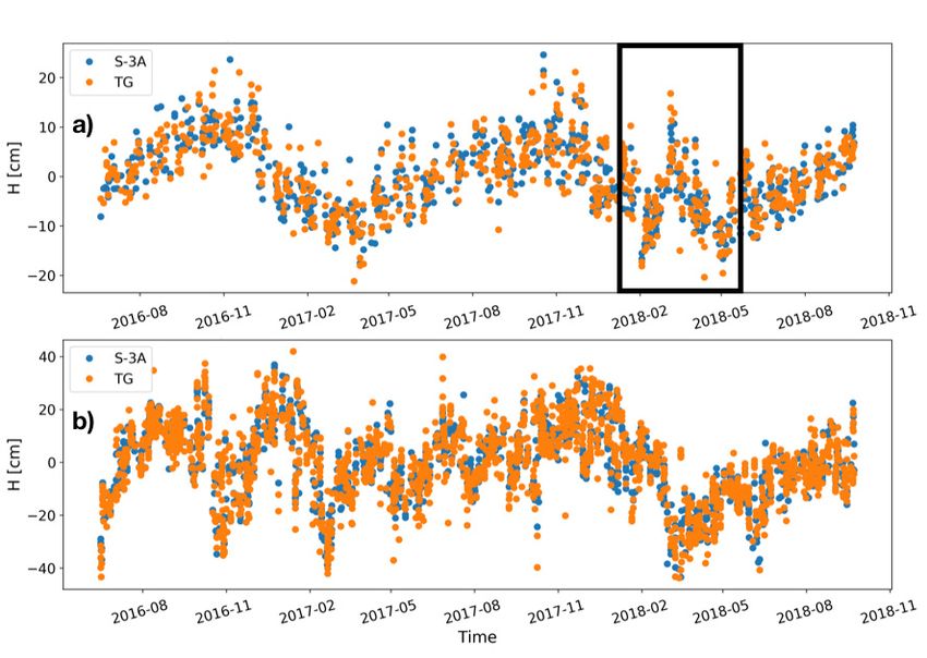
Remote Sens. 2020, 12, 3970                                                                            2 of 27

      In parallel with these efforts, the Sentinel-3A satellite was launched in February 2016 as part of
the European Union Copernicus Programme. It became fully operational in July 2016. The Sentinel-3
mission is jointly operated by the ESA and the European Organisation for the Exploitation of
Meteorological Satellites (EUMETSAT) to deliver, among other things, operational ocean observation
services [11]. The Sentinel-3A onboard altimeter, a synthetic aperture radar altimeter (SRAL), is based on
a principle proposed by [12]: the synthetic aperture radar mode (SARM). The SRAL has two advantages
over the conventional altimeter: (i) a finer spatial resolution in the along-track dimension [13] and (ii) the
higher signal-to-noise ratio of the received signal and lower speckle noise from SAR waveforms [14,15],
providing enhanced Sea Level Anomaly (SLA) measurements in the coastal zone [15].
      The Sentinel-3A data are processed by EUMETSAT (https://www.eumetsat.int), which freely
distributes level 1 and level 2 products. These products are in a second step reprocessed through the
Data Unification and Altimeter Combination System (DUACS) altimeter multi-mission processing
system (https://duacs.cls.fr). The DUACS system provides directly usable, high-quality near-real-time
and delayed time (DT) global and regional altimeter products [1,5]. The main processing steps
include product homogenisation, data editing, orbit error correction, reduction in Long Wavelength
Errors (LWE), and the production of along-track and mapped sea level anomalies. The DUACS
processing [3] is based on the altimeter standards given by L2P (Level-2 Plus) products (see e.g., [16]).
They include the most recent standards recommended for altimeter global products by agencies and
expert groups such as the Ocean Surface Topography Science Team (OSTST) and the ESA Quality
Working groups.
      More than 25 years of level-3 (L3) and level-4 (L4) altimetry products were reprocessed and
recently delivered as the DUACS DT 2018 version [5]. L3 products for repetitive altimeter missions
are based on the use of a mean profile [3,17] that allows collocating the SSH of the repetitive tracks
and retrieving a precise mean reference to compute SLAs [5]. SLAs are often used instead of absolute
dynamic topography, defined as the differences between SSH and the geoid height, because the geoid
is not perfectly known at scales smaller than 150 km from space gravity missions [17]. To solve this,
a mean sea surface model based on altimetry data that contains the sum of the geoid height and the
mean dynamic topography is used [17].
      The along-track SLA products are affected by the uncertainties in the geoid surface model and also
by (i) instrumental errors, (ii) environmental and sea state errors, and (iii) the precision of geophysical
corrections. These elements introduce errors in the measurements [18]. To minimise their impact,
DUACS-DT2018 re-processing considers the most up-to-date altimetry corrections, such as (a) dry
and wet troposphere corrections, (b) ionospheric correction, (c) sea state bias correction, (d) dynamic
atmospheric correction (DAC), and (e) the ocean tide. Some of these instrumental and environmental
errors remain in the along-track products delivered to final users, mainly due to the imprecision of the
corrections applied.
      Altimeter data are widely calibrated and validated by comparison with in situ timeseries [19].
Tide gauge measurements are commonly used. In situ and altimetric observations are complementary
and are often assumed to observe the same signals (e.g., [20]). The comparisons with in situ observations
allow us to obtain altimetry errors relative to the external measurements and provide an improved
picture of SSH. The paper [5] assessed gridded products in coastal areas through a comparison
with monthly tide gauge measurements from the Permanent Service for Mean Sea Level (PSMSL)
Network [21]. The procedure described in [19,22] was used. The paper [5] reported a global reduction
of 0.6% in variance when using the DUACS-DT2018 data with respect to the previous DUACS-DT2014
dataset [3], with a clear improvement along the Indian coast, Oceania, and Northern Europe.
      The consistency between altimeter gridded products and tide gauge data in the coastal region
was also investigated at global [23,24] and regional (Mediterranean basin) scales [25,26]. Mean square
differences between tide gauge and gridded altimetry (see Section 3.1 in the text) ranging between
30% and 90% were obtained by [23] in the European coasts, whilst these differences were reduced to
around 40% [24] thanks to improved geophysical corrections (i.e., a new DAC) applied to altimetry
Remote Sens. 2020, 12, 3970 3 of 27
data with root mean square differences (RMSD) between gridded altimetry and tide gauges of 4.43 cm
in the Atlantic Ocean. The paper [25] found a median value for the correlation altimetry—a tide gauge
of 0.79 in the Mediterranean Sea.
These works used low-pass filtered (monthly averaged) tide gauge records from PSMSL and the
Global Sea Level Observing System (GLOSS)/Climate Variability and Predictability (CLIVAR) [27] to
remove high frequencies not resolved by the altimetry gridded products used for inter-comparisons.
Thus, a comparison at higher frequencies between a specific regional product for the whole European
coast and a high-density tide gauge dataset is, to our knowledge, still lacking.
Here, we present an assessment of the Copernicus Marine Environment Monitoring Service
(CMEMS)/DUACS along-track (L3) altimeter regional operational products in the European seas using
in situ tide gauges from the Copernicus Marine Environment Monitoring Service (CMEMS) catalogue.
The aim is to validate the Sentinel-3A SAR mode SLAs against the equivalent in situ tide gauge
measurements. Six-hour time series of tide gauge measurements will be compared with the 1 Hz
along-track altimetry data from the Sentinel-3A satellite mission, this strongly enhancing both the
spatial and temporal resolution of the results reported by [5]. We expect to obtain a more detailed
assessment of DUACS-DT2018 products in the European seas at the both regional and sub-regional level.
This inter-comparison has been also conducted by using SLA from the Jason-3 satellite mission to
investigate the improvements of the Sentinel-3A mission over the latter in the coastal band.
2. Materials and Methods
2.1. Sea Level Anomalies from Altimetry
The DUACS-DT2018 along-track (L3) regional altimetry products for the European seas were
released by cmEMS in 2018. We use delayed-time (quality controlled) reprocessed altimeter along-track
SLA products computed with respect to a twenty-year (1993–2012) mean for the satellite missions
Jason-3 and Sentinel-3A. These products have a spatial sampling of around 7 km, corresponding
to the upstream 1 Hz products sampling. Filtered and unfiltered SLA measurements are provided.
In this work, we have used both. Unfiltered SLA is the raw SLA (i.e., not filtered) measured by the
instrument. Unless otherwise stated, SLA will refer to unfiltered SLA throughout the text, except for
Section 3.3, where we specifically compare the results obtained from both SLAs.
Filtered SLA is computed for regional Europe products in the DUACS procedure by applying a
Lanczos low-pass filter with a cut-off wavelength of around 40 km to SLA measurements (e.g., [13]).
The aim is to remove the noise signal and the short wavelengths affected by the noise [18]. This procedure
is discussed in [3]. This low-pass cut-off length is the minimal one that can be applied to along-track
SLA to reduce noise effects and preserve as much as possible the physical signal. Filtered SLA is
not sub-sampled to keep the 1 Hz full resolution. We decided to focus on the reference low-rate
(1 Hz) SLAs instead of high-rate (i.e., 20 Hz) SLAs, because the former are produced by DUACS and
delivered by cmEMS to the entire oceanographic community. The high-frequency 20 Hz products are
not available for most users. Figure 1 shows a flowchart explaining the DUACS procedure applied to
the altimetry data.
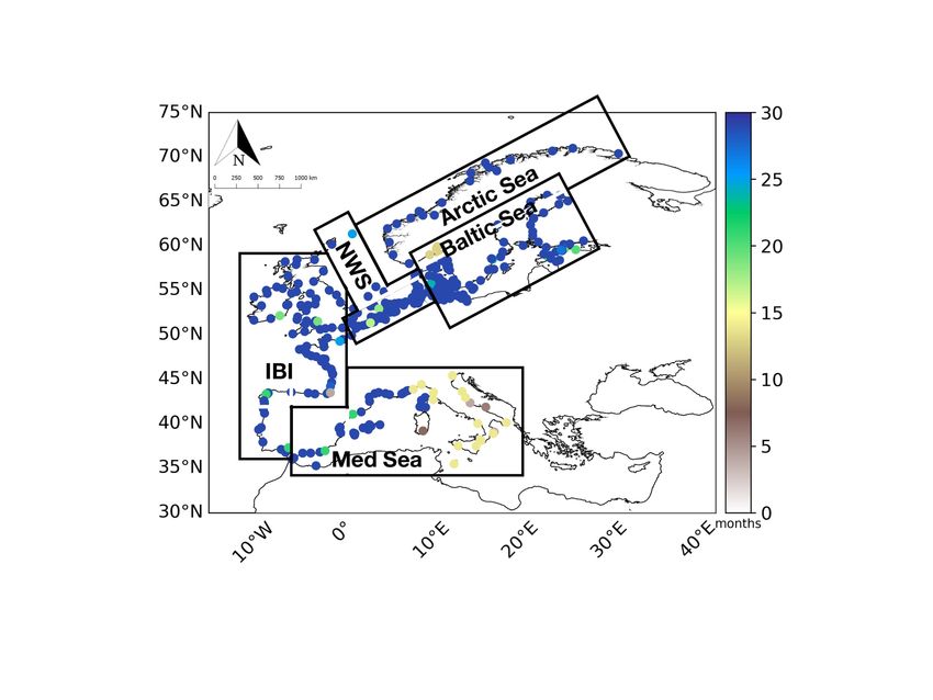
The time period analysed spans from May 2016 to September 2018. The areas investigated
are the whole European coast, the Baltic Sea, the Arctic Sea, North-West Shelves (NWS) region,
the Iberian-Biscay-Irish (IBI) region, and the central-western Mediterranean Sea (Figure 2).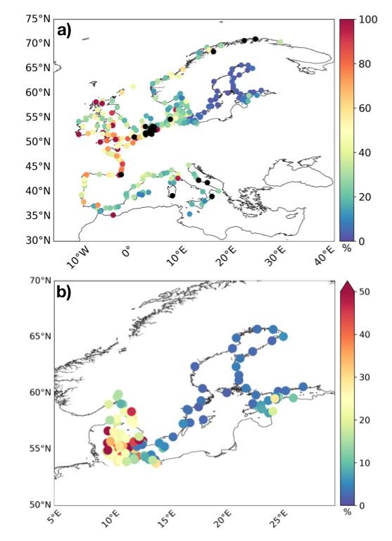
Remote Sens. 2020, 12, 3970                                                                                      4 of 27
Remote Sens. 2020, 12, x FOR PEER REVIEW                                                                         4 of 35

     Figure
     Figure 1. Flowchart of
            1. Flowchart  of the
                             the Data
                                 Data Unification
                                      Unification and
                                                  and Altimeter
                                                       Altimeter Combination
                                                                  Combination System
                                                                               System (DUACS)
                                                                                      (DUACS) procedure
                                                                                                procedure
     applied
     applied to
             to altimetry
                altimetry data
                          data and
                               and the
                                   the processing
                                       processing of
                                                   of the
                                                      the tide
                                                          tide gauge
                                                               gauge data
                                                                     data used
                                                                          used to
                                                                               to compare
                                                                                  compare with
                                                                                          with altimetry.
                                                                                               altimetry.

     Figure 2. Location of the 370 tide gauges of the global product in the Copernicus catalogue along the
     European coasts and the western Mediterranean Sea used to compare with altimetry data after
     applying the selection criteria described in the text. Colours indicate the length of the time series of
     the concurrent tide gauge data and altimeter data. The black squares denote the sub-regions used for
     the inter-comparisons (see the text for details).

2.2. Tide Gauge Observations
     Figure 2. Location of the 370 tide gauges of the global product in the Copernicus catalogue along
     TheEuropean
     the  sea-levelcoasts
                     recordsandused    to compare
                                 the western          with satellite
                                                Mediterranean        altimetry
                                                                 Sea used        were with
                                                                           to compare   obtained   fromdata
                                                                                              altimetry   the after
                                                                                                               CMEMS
In Situ Thematic
     applying      Assembly
              the selection       Centre
                             criteria       (TAC)
                                      described  in data  repository.
                                                    the text.           The Copernicus
                                                              Colours indicate the length ofcatalogue   provides
                                                                                             the time series of the data
of 485 tide gauge
     concurrent tidestations  along
                      gauge data    andthe  Worlddata.
                                         altimeter   OceanThecoasts, which are
                                                              black squares      updated
                                                                             denote         within aused
                                                                                     the sub-regions  few weeks
                                                                                                            for the or a
few months.    This dataset
     inter-comparisons          covers
                         (see the         the
                                   text for   time period spanning from January 2010 to the present. Six-
                                            details).
hourly tide gauge records were used according to the following procedure (Figure 1): the 445 tide
gauge stations located in the European seas’ domain were initially considered for this study. The
quality flags of the tide gauge records were checked and observations with anomalous SSH data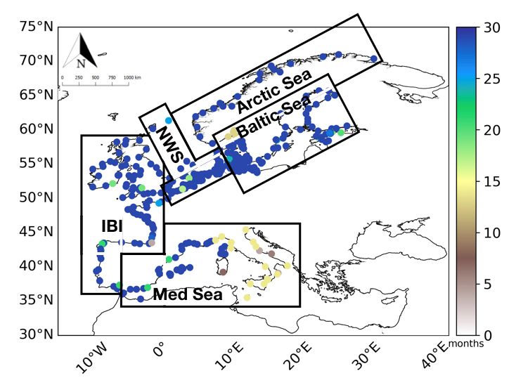
Remote Sens. 2020, 12, 3970                                                                         5 of 27

2.2. Tide Gauge Observations
      The sea-level records used to compare with satellite altimetry were obtained from the cmEMS
In Situ Thematic Assembly Centre (TAC) data repository. The Copernicus catalogue provides data
of 485 tide gauge stations along the World Ocean coasts, which are updated within a few weeks or a
few months. This dataset covers the time period spanning from January 2010 to the present. Six-hourly
tide gauge records were used according to the following procedure (Figure 1): the 445 tide gauge
stations located in the European seas’ domain were initially considered for this study. The quality flags
of the tide gauge records were checked and observations with anomalous SSH data (values larger than
three times the standard deviation of the time series) or changes in the vertical reference of the tide
gauge were rejected. Additionally, tide gauge time series exhibiting a large variance (more than 20 cm2 )
with respect to altimetry data were removed, as they are considered not representative of ocean sea
level changes and are likely related to local features (e.g., river discharge). Only tide gauges with at
least a 70% yearly data coverage were selected in order to allow the analysis of the seasonal signal.
      The final set consists of 370 stations (Figure 2). The stations and their information are listed in
Table A1. Before they can be compared with altimeter data, tide gauge measurements have to be
processed [7,19] to remove oceanographic signals whose temporal periods are not resolved by altimetry,
thus avoiding important aliasing errors [6]. First, tidal components were removed from the sea level
records using the u-tide software [28]. The annual and semiannual frequencies, mainly driven by
steric effect, are kept in the tidal residuals since they are included in the altimetry data.
      For consistency with the satellite altimetry data, the atmospherically induced sea level caused
by the action of atmospheric pressure and wind was removed from the tidal residuals [7,25,29].
This high-frequency oceanic signal is badly sampled by altimeter measurements. To solve this problem,
a combination of high frequencies of a barotropic model forced by pressure and wind (MOG2D)
and low frequencies of a classical Inverted Barometer model was applied [30]. We used the DAC
available at the Archiving, Validation, and Interpretation of Satellite Oceanographic Data (AVISO)
website. The DAC data are provided as 6 h sea level fields on a 1/4◦ × 1/4◦ regular grid covering the
global oceans. For each tide gauge site, the nearest grid point was selected and used to remove the
atmospherically induced sea level from observations, previously converted into 6-hourly records [25].
Finally, the 6-hourly tidal residuals were corrected for vertical movements associated with glacial
isostatic adjustment (GIA). Indeed, many studies have demonstrated the need for tide gauges to be
corrected for vertical crustal land motion when compared to altimeter data, since tide gauges measure
the relative sea level with respect to the land where they are grounded [19]. We considered GIA as the
only source of vertical land motions and removed its effects from the tidal residuals using the Peltier
mantle viscosity model (VM2) [31,32].

2.3. Method for Comparing Altimeter and In Situ Tide Gauge Records
     The comparison method of altimetry with tide gauges consisted of co-locating both datasets in
time and space. It was based on a particular track point selected for each tide gauge location as follows:
we computed the correlations between each tide gauge record (tidal residuals) and SLA time series
corresponding to track points within a radius of 1 degree around the tide gauge site and choose
the most correlated track point. A minimum length of time series of 10 months (corresponding to
approximately 10 cycles of Sentinel-3A) was set up to allow statistical significance [14]. Statistical
analyses were performed between both datasets using all available data pairs (altimetry-tide gauge)
for a given region.
     The co-located altimeter and tide gauge measurements were analysed in terms of the RMSD and
variance of the time series. The RMSD metric is commonly used to examine along-track altimeter
data quality [14]. In addition, the robustness of the results was investigated according to [33] using
a bootstrap method [34], which allows us to estimate quantities related to a dataset by averaging
estimates from multiple data samples. To do that, the dataset is iteratively resampled with replacement.
A total of 103 iterations were used to ensure that meaningful statistics such as standard deviation could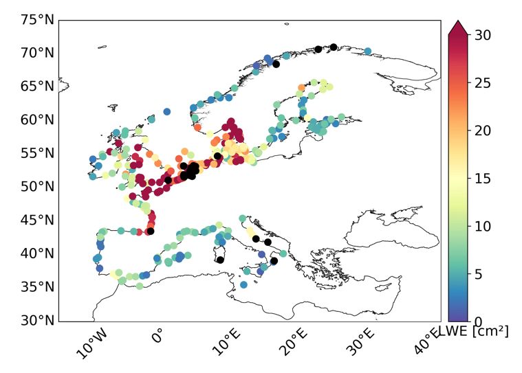
Remote Sens. 2020, 12, 3970                                                                        6 of 27

be calculated on the sample of estimated values, thus allowing us to assign measures of accuracy to
sample estimates.

2.4. Ancillary Data
     The Global, Self-consistent, Hierarchical, and High-resolution Geography database (GSHHG)
was used to estimate the nearest distance to the coast of the altimetry track points used to compare
with tide gauges. The aim was to investigate the degradation of the altimetric signal as we approach
the coast. The shorelines in the GSHHG database are constructed entirely from hierarchically arranged
closed polygons and are available in five geographical resolutions. The early processing and assembly
of the shoreline data is described in [35]. We used the latest data files for version 2.3.7 presently
available and released on 15 June 2017 with the original full data resolution.

3. Results

3.1. Comparison of Sentinel-3A and Tide Gauges along the European Coasts
      This section presents the statistics of the comparisons performed between the Sentinel-3A altimetry
data and the tide gauge observations from the cmEMS catalogue in the coastal region in terms of errors
(RMSD) and the variance of the differences between both datasets. The analysis has been conducted
for the entire European coast and the following sub-regions: the Mediterranean Sea, the IBI and
NWS regions, and the Baltic Sea (Figure 2). SLA measurements without filtering (Figure 1) were used.
The bootstrapping technique [34] was applied to gain an estimation of the standard errors of the
differences between both datasets.
      The mean value of the RMSD between the Sentinel-3A satellite altimetry and tide gauges is
6.97 cm. The mean distance between the location of the tide gauge and the location of the corresponding
altimeter data with the highest correlation is 80 km with a standard deviation of 33 km. Data from
342 tide gauge stations were compared with the Sentinel-3A data. Thus, 28 stations were rejected from
the computation according with the selection criteria described in the previous section. These stations
are located in the NWS region, the Mediterranean Sea, and the Arctic Sea (Table A1).
      The rejected tide gauge time series showing a variance much larger than that found in the
corresponding altimetry time series (RMSD between both datasets larger than 20 cm) were further
investigated. We checked the shape of their time series, together with the quality flag data related
to SSH, tide gauge position, and recorded atmospheric pressure. The aim was to investigate the
presence of outliers in the tide gauge time series due to poor quality control not captured by satellite
altimetry responsible for such large discrepancies, which could be corrected by the data providers.
A subset of twenty-four tide gauge stations (Table A2) showed abnormal values in variance due to
poor quality control that induced substantial RMSD when compared to the Sentinel-3A and Jason-3
altimetry data. This represents 5% of the tide gauge dataset in the European coasts.
      Figure 3 shows the consistency between the altimetry and tide gauge data computed as follows:

                               variance(tide gauge − altimeter)
                                                                × 100,                                (1)
                                    variance(tide gauge)

where the variance of the tide gauge is associated with the variance of the signal. Consistency is
expressed here as the mean square differences between both datasets, computed as the variance of the
differences (altimetry—tide gauge) in terms of percentage of the tide gauge variance. This approach
has already been applied by [23,24] to compare the satellite altimetry and tide gauge measurements at
a global scale.
     Overall, mean square differences lower than 10% are observed in most of the Baltic Sea (Figure 3b).
Larger mean square differences of around 25% are observed in the Gulf of Finland, whereas they
reach values between 15% and 50% and even larger values when in connection region with the North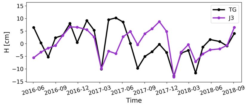
Remote Sens. 2020, 12, 3970                                                                                         7 of 27

Atlantic Ocean. The mean square differences are between 20% and 50% for stations located in the
 Mediterranean Sea and the NWS region (Figure 3a).
       If we analyse the results in terms of the RMSD (figure not shown), minimum mean errors of 3.41 cm
were obtained in the Mediterranean Sea, whilst they increased until 10.72 cm for the NWS region.
These results can be explained by the larger spatio-temporal variability observed in the NWS region
(SLA mean variance of 206 cm2 ) with respect to that found in the Mediterranean basin (SLA mean
 variance of 47 cm2 ). Non-tidal variance, which is also larger in the former [36], contributes to the larger
Remote
 RMSD   Sens. 2020, 12, in
          obtained      x FOR
                           the PEER
                               NWSREVIEW
                                    region.                                                            7 of 35

      Figure 3. Spatial distribution of the mean square differences between the tide gauge and altimetry sea
     Figure 3. Spatial distribution of the mean square differences between the tide gauge and altimetry sea
      level from Sentinel-3A in the European coasts (panel (a)). Black dots denote the location of the tide
     level from Sentinel-3A in the European coasts (panel (a)). Black dots denote the location of the tide
      gauge sites rejected from the computation according with the selection criteria described in the text.
     gauge sites rejected from the computation according with the selection criteria described in the text.
      Panel (b) shows a detailed view of the Baltic Sea region. Sea Level Anomaly (SLA) measurements
     Panel (b) shows a detailed view of the Baltic Sea region. Sea Level Anomaly (SLA) measurements
      without filtering have been used. Units are the percent of tide gauge variance.
     without filtering have been used. Units are the percent of tide gauge variance.
      The largest errors, which reach 100%, are mainly found in the Atlantic shore of the IBI region.
3.2.
 This could be dueoftoSentinel-3A
     Improvements                 over Jason-3
                       the imprecisions   of theSatellite Mission
                                                 corrections   applied (i.e., ocean tide) to the altimeter data.
      In this section, we conduct an equivalent analysis on Jason-3 data. The Jason-3 satellite mission
 3.2. Improvements of Sentinel-3A over Jason-3 Satellite Mission
has an orbit repeat cycle of 9.91 days, whilst Sentinel-3A presents a repeat cycle of 27 days. To make
       In this section, we conduct
the inter-comparisons          betweenanboth equivalent
                                                  satelliteanalysis
                                                              missionson Jason-3
                                                                           with indata.situThe  Jason-3
                                                                                             tide  gauge satellite mission
                                                                                                            observations
 has an orbit repeat
comparable,       SLA fromcycleJason-3
                                 of 9.91 days,  whilst Sentinel-3A
                                         was sub-sampled                 presents
                                                                 to retain   everya third
                                                                                     repeatpoint
                                                                                              cycle along
                                                                                                    of 27 days.   To make
                                                                                                           the tracks    to
 the inter-comparisons
emulate    the Sentinel-3A   between
                                  cycle.both
                                          Thesatellite  missions
                                               tide gauge          with in
                                                               stations     situstations)
                                                                          (270   tide gauge    observations
                                                                                            common            comparable,
                                                                                                        to both   satellite
 SLA from
missions       Jason-3
            were    used.was    sub-sampled
                           The results   obtainedto for
                                                     retain  every third
                                                         the whole           pointcoasts
                                                                      European       alongarethe  tracks to emulate
                                                                                               summarised     in Table the
                                                                                                                        1.
 Sentinel-3A
      Notice thatcycle.  The
                       the    tide gauge
                           rejected   tide stations   (270 stations)
                                           gauge stations      in thecommon       to both satellite
                                                                        inter-comparison             missionsare
                                                                                              with Jason-3      were  used.
                                                                                                                   mainly
 The results
located        obtained
          in the   central for
                            partthe
                                  of whole  European coasts
                                     the Mediterranean      Sea,are
                                                                  thesummarised       in Table
                                                                       Gulf of Finland,         1.
                                                                                           the easternmost     part of the
BalticNotice
        Sea, andthatalong
                      the rejected
                            most oftide
                                      thegauge   stationscoast.
                                           Norwegian       in theAs
                                                                  inter-comparison
                                                                      a consequence with      Jason-3
                                                                                         of this,      are mainly
                                                                                                  the Arctic       located
                                                                                                              region  will
 in the
not     central part ofhere
     be investigated       the due
                                Mediterranean     Sea,
                                     to the lack of     the Gulf
                                                     valid         of Finland,
                                                            data (Figure    A1).the easternmost part of the Baltic Sea,

     Table 1. Inter-comparison of the satellite altimetry and tide gauge data from the European coasts in
     terms of the RMSD (cm) and variance (cm2) of the differences between both datasets. The number of
     tide gauge stations used in the comparison, the mean distance between tide gauges and the most
     correlated along-track altimetry points, and the number of total data pairs (altimetry-tide gauge) used
Remote Sens. 2020, 12, 3970 8 of 27
and along most of the Norwegian coast. As a consequence of this, the Arctic region will not be
investigated here due to the lack of valid data (Figure A1).
The RMSD between the Jason-3 and tide gauge time series shows a mean value of 7.97 cm,
whereas it is reduced to 6.89 cm for the inter-comparison using the Sentinel-3A dataset. Overall,
the results from the Jason-3 satellite mission are consistent with those obtained for Sentinel-3A in terms
of spatial distribution (Figure A1).
In the IBI and NWS regions, 81 and 55 common tide gauge stations to Sentinel-3A and Jason-3
missions were respectively identified from the whole tide gauge dataset (Table 2). The analysis
conducted with these stations shows a mean RMSD of 6.62 cm and 10.31 cm, respectively, for the
comparison with Sentinel-3A, whilst the mean values for the inter-comparison using the Jason-3 dataset
are 7.31 cm for the IBI region and 12.22 cm for the NWS region. Thus, the Sentinel-3A satellite mission
improves, respectively, the errors with tide gauges in both regions by 9% and 15%.
Table 1. Inter-comparison of the satellite altimetry and tide gauge data from the European coasts in
terms of the RMSD (cm) and variance (cm2 ) of the differences between both datasets. The number
of tide gauge stations used in the comparison, the mean distance between tide gauges and the most
correlated along-track altimetry points, and the number of total data pairs (altimetry-tide gauge) used
in the computation are displayed. The common tide gauge stations for the Sentinel-3A and Jason-3
satellite missions were used. Values in parenthesis show the uncertainties (error bars) computed for
the RMSD and variance from the bootstrap method using 103 iterations. Finally, the improvement (%)
of the Sentinel-3A data in comparison with tide gauges in terms of lower RMSD, lower variance of
the differences (altimetry-tide gauge), and lower mean distance between the most correlated altimetry
point and tide gauges with respect to Jason-3 is also displayed. SLA measurements without filtering
have been used.
European Coasts Sentinel-3A Jason-3 Improvement
RMSD (cm) 6.89 (0.17) 7.97 (0.21) 13%
var TG (cm2 ) 150 (6) 138 (5)
var ALT (cm2 ) 124 (5) 117 (5)
var TG-ALT (cm2 ) 47 (3) 64 (3) 25%
data pairs 6037 6172
stations 270 270
distance TG (km) 79 ± 33 87 ± 33 9%
In the Baltic and Mediterranean seas (Table 2), where generally lower errors are observed,
we identified, respectively, 88 and 38 tide gauge stations common to both missions, showing a mean
RMSD of 5.69 cm and 3.47 cm for the comparison with Sentinel-3A, whilst the mean values for the
inter-comparison using the Jason-3 data are 6.24 cm and 4.49 cm, respectively. Thus, the Sentinel-3A
satellite mission improves the errors with tide gauges in both regions by 9% (23%) in the Baltic
(Mediterranean) Sea.
Notice that the mean distance between tide gauge sites and the most correlated altimetry track
points is shorter for the Sentinel-3A mission in all the sub-basins investigated except for the Baltic Sea,
where the same mean distance is obtained for both satellite missions (Table 2). At first sight, this fact
may contribute to the better results obtained for the Sentinel-3A mission. However, a shorter distance
between tide gauge and the altimeter co-location point does not always result in a lower RMSD
and variance of the differences (tide gauge—altimetry). This fact can be observed in the Baltic Sea,
where an overall improvement of Sentinel-3A over Jason-3 is found despite the same mean distance
tide gauge—altimetry for both missions. Therefore, this parameter has not a strong impact on the
better results obtained with Sentinel-3A, and other reasons for the higher performance of the SAR
technology in the coastal zone must be given.
To further investigate the impact of SAR technology on the quality of the Sentinel-3A data close to
the coast, we analyse in the following sections how the measurement noise and the approach to the
coast affect the retrieval of SLA in both the Sentinel-3A and Jason-3 missions. Moreover, the impact ofRemote Sens. 2020, 12, 3970 9 of 27
the LWE processing, associated with geographically correlated errors between neighbouring tracks
from different sensors, on the quality of altimetry along-track products will be assessed. The LWE is an
empirical correction that aims at removing residual ocean tide and DAC signal, as well as residual
orbit error (residual signals induced by the imperfection of the solution used for these corrections).
Table 2. The same as Table 1 but for the different sub-regions investigated: Mediterranean Sea,
Iberian-Biscay-Irish (IBI) region, North-West Shelves (NWS) region, and Baltic Sea.
Sub-Regions Sentinel-3A Jason-3 Improvement S-3A
Mediterranean Sea
RMSD (cm) 3.47 (0.22) 4.49 (0.28) 23%
var TG (cm2 ) 53 (5) 46 (4)
var ALT (cm2 ) 52 (5) 49 (4)
var TG-ALT (cm2 ) 12 (1) 20 (3) 40%
data pairs 743 836
stations 38 38
distance TG (km) 67 ± 30 74 ± 40 9%
IBI region
RMSD (cm) 6.62 (0.30) 7.31 (0.28) 9%
var TG (cm2 ) 72 (5) 63 (4)
var ALT (cm2 ) 56 (4) 51 (4)
var TG-ALT (cm2 ) 44 (4) 53 (4) 18%
data pairs 1927 1920
stations 81 81
distance TG (km) 80 ± 30 89 ± 33 10%
NWS region
RMSD (cm) 10.31 (0.53) 12.22 (0.60) 15%
var TG (cm2 ) 268 (22) 264 (20)
var ALT (cm2 ) 201 (18) 185 (16)
var TG-ALT (cm2 ) 106 (11) 149 (14) 29%
data pairs 1256 1416
stations 55 55
distance TG (km) 84 ± 35 101± 27 17%
Baltic Sea
RMSD (cm) 5.69 (0.28) 6.24 (0.28) 9%
var TG (cm2 ) 217 (13) 199 (12)
var ALT (cm2 ) 190 (11) 184 (12)
var TG-ALT (cm2 ) 32 (3) 39 (3) 17%
data pairs 1940 1856
stations 88 88
distance TG (km) 78 ± 33 78 ± 31 —
3.3. Impact of the Measurement Noise on the Retrieval of SLA in the Coastal Area
To check the impact of the measurement noise on the SRAL instrument onboard the
Sentinel-3A mission, the inter-comparison between satellite altimetry and in situ tidal records in the
European coasts is repeated but using the Lanczos low-pass filtered SLA available in cmEMS altimetric
products (Section 2.1 and Figure 1). The outcomes are then compared with the inter-comparison
conducted in the previous section. The same tide gauge sites and data points for the inter-comparisons
using filtered SLA and SLA measurements without filtering from the Sentinel-3A mission were used to
make the outcomes comparable. As a consequence, the statistics for the SLA measurements displayed
in Table 3 slightly differ from those shown in Table 1 due to the different tide gauge sites and data
pairs used.
The variance of the Sentinel-3A altimetry data diminished by 2% when using the filtered data
(Table 3). This is an expected result due to higher frequencies being subtracted from the SLA time series
in the filtering procedure. This fact decreased the RMSD by 0.3% when comparing the filtered SLA withRemote Sens. 2020, 12, 3970 10 of 27
tide gauge records with respect to that obtained when using the SLA without filtering. The variance of
the differences (altimetry—tide gauge) was also reduced by 1% when using the Sentinel-3A filtered data.
However, it is worth noting that the improvements in the inter-comparisons (RMSD reduction) when
using filtered SLA are negligible.
Table 3. The same as Table 1 but for the inter-comparison using Lanczos low-pass filtered SLA and
SLA measurements without filtering for the Sentinel-3A and Jason-3 satellite missions. Common tide
gauge stations for each satellite mission have been used.
Improv.
European Coasts Sentinel-3A Improv. Jason-3
Filtered J-3
Filtered S-3A
Unfiltered Filtered Unfiltered Filtered
RMSD (cm) 6.97 (0.19) 6.95 (0.19) 0.3% 8.72 (0.25) 8.52 (0.25) 2.3%
var TG (cm2 ) 149 (5) 146 (6)
var ALT (cm2 ) 121(7) 119 (7) −2% 121 (5) 114 (5) −6%
var TG-ALT (cm2 ) 49 (3) 48 (3) 1% 76 (4) 72 (4) 5%
data pairs 7119 6228
stations 340 277
distance TG (km) 80 ± 36 87 ± 34
This procedure was repeated using the Jason-3 dataset (Table 3). A reduction threefold larger (6%)
in the variance of the filtered SLA with respect to the SLA without filtering is observed. This underscores
the expected larger measurement noise in the unfiltered SLA from the Jason-3 Low Resolution Mode
mission compared to the SAR mission [37,38]. As a result, a reduction of 2.3% in the RMSD was
obtained when using filtered data. Additionally, the variance of the differences (altimetry—tide gauge)
diminished by 5% when using the Jason-3 filtered data.
3.4. Effects of the Coastal Distance on Altimeter Data
The quality of retrieved altimeter signal decays with closer distance to the coast, because radar
return from the land and bright target causes the typical shape of waveform to deviate [14,39].
To investigate the degradation of the altimeter signal and its performance as we approach the coast,
an additional comparison between satellite altimetry from both Sentinel-3A and Jason-3 and in situ
tidal records in the European coasts was conducted.
First, we estimated the distance to the coast of all track points within a radius of 1 degree around
a given tide gauge by using the GSHHG dataset. Then, the closest altimetry track point to the coast
(ctp hereafter) and the most correlated altimetry point (mcp hereafter) along the track of the ctp
were identified. This provides two altimeter time series from track points along the same track from a
given mission but with a different or equal distance to the coast (the latter if ctp and mcp match up)
to compare against the same tide gauge. SLA measurements without filtering (Figure 1) were used.
Finally, statistics (RMSD and variance) for the inter-comparisons of satellite ctp and mcp with tide
gauges were obtained. Differences between statistics when using the altimetry mcp and ctp against the
same tide gauge will provide an estimation of the degradation of the altimetry signal as we approach
the coast.
To obtain comparable results between the Sentinel-3A and Jason-3 missions, tide gauge sites
exhibiting altimetry ctp with a similar distance to coast for both missions were identified. A maximum
difference for the distance to the coast of ctp from the Sentinel-3A and Jason-3 missions for a given tide
gauge site of 1 km was allowed. Only tide gauge sites showing a distance to coast of the altimetry mcp
lower than 40 km were kept. This ensures the analysis in the nearest coastal zone of the European Seas,
where the data quality can be affected by the impact of land and islands near the coast. Twenty-seven
common tide gauge stations keeping the aforementioned selection criteria were identified.
Overall, the inter-comparisons between SLA measurements and tidal residuals improved in
terms of RMSD and variance when using the altimetry mcp time series for both missions. This is anRemote Sens. 2020, 12, 3970 11 of 27
expected result, although the altimetry ctp is located closer to tide gauges and also closer to coast than
the altimetry mcp for both missions (Table 4).
Table 4. The same as Table 1 but for the inter-comparison using the altimetry closest track point to coast
(ctp) and the most correlated altimetry point (mcp) with tide gauge records computed along the satellite
track of ctp (see text for details) for the twenty-seven common tide gauge stations showing a similar
distance with the altimetry ctp for Sentinel-3A and Jason-3 (a maximum difference of 1 km is allowed).
The distance (km) of mcp and ctp to both tide gauges (TG) and coast and the degradation (in percentage)
of the altimetry signal, computed as the differences between mcp and ctp, are also shown.
Sentinel-3A Jason-3
European Coasts Degrad. S-3A Degrad. J-3
mcp ctp mcp ctp
RMSD (cm) 6.78 7.95 7.91 8.74 15% 10%
var TG (cm2 ) 173 172
var ALT (cm2 ) 121 127 125 139 5% 10%
var TG-ALT (cm2 ) 62 80 81 101 22% 20%
distance TG (km) 60 46 87 75 23% 14%
distance coast
13.5 5.1 12.2 5.4 62% 56%
(km)
data pairs 456 442
stations 27
The mean distance to tide gauges is lower for the Sentinel-3A dataset for both the mcp and ctp due
to the reduction in the cross-track distance in the Sentinel-3A orbit with respect to Jason-3. The RMSD
increased from 6.78 cm to 7.95 cm when we approach the coast (from the mcp location to the ctp
location) for the Sentinel-3A dataset and from 7.91 cm to 8.74 cm for the Jason-3 dataset. These results
suggest an impact of the distance to coast on the data quality for both missions.
The degradation of the altimeter signal, estimated here as the difference in the percentage of
statistics between the altimetry mcp and ctp computations for a single mission, shows a mean value
for the RMSD of 15% for the Sentinel-3A mission when we approach the coast from around 13 km
to 5 km and of 10% for the Jason-3 mission. The degradation in the variance of the differences
(altimetry—tide gauge) was 22% for Sentinel-3A and 20% for the Jason-3 dataset. Despite this lower
degradation in the Jason-3 dataset, a superior performance of the Sentinel-3A dataset in terms of the
lower along-track RMSD and a lower variance of the differences (altimetry—tide gauge) against the
same tide gauges was obtained, also showing a mean distance of the ctp 300 m closer to coast than that
of the Jason-3 dataset (Table 4). The number of points used for both altimeters is similar, at 456 for
Sentinel-3A and 442 for Jason-3, this suggesting a reasonable comparison.
The altimetry variance exhibited an enhancement of 5% for the Sentinel-3A dataset when we
approached the coast, whilst it reached 10% for the Jason-3 mission (Table 4). This twofold increase in
the latter can be associated with a larger impact of the measurement noise on altimeters onboard the
Jason-3 close to coast, as was shown in the previous section. This fact again confirms that the SRAL
instrument better solves the signal in the coastal band.
3.5. Impact of the Long Wavelength Error Correction Applied on Satellite Altimetry
SLA in DUACS-DT2018 processing is provided to data users after removing several disturbances
affecting the altimeter measurements such as high-frequency oceanic signals, ocean tides, and Long
Wavelength Error correction (LWE). The LWE is an empirical correction that aims at removing residual
ocean tide and DAC signal as well as residual orbit error. An LWE reduction algorithm based on
Optimal Interpolation (see for instance [1,3]) is applied. This optimal-interpolation based empirical
correction contributes to remove high-frequency variability in the altimetry SLA due to noise (errors in
corrections) and high-frequency signals close to the coast that are not fully corrected by the application
of the corrections to minimise the other two aforementioned errors [40].Remote Sens. 2020, 12, 3970 12 of 27
In this section, we investigate the possible impact of the LWE correction applied to Sentinel-3A
and Jason-3 datasets on both the retrieval of SLA in the coastal zone and the inter-comparisons with in
situ measurements performed. To do that, LWE correction applied to SLA was subtracted from the
altimetry time series to obtain uncorrected SLA as follows:
SLAuncorr = SLA − LWE (2)
Then, the SLAuncorr time series were compared with tide gauge records according to the procedure
described in previous sections. Finally, the outcomes from this new computation were compared
with the inter-comparison conducted by using the corrected SLA. In this analysis, SLA measurements
without filtering have been used.
RemoteThe
Sens.variance
2020, 12, x FOR PEER REVIEW
associated with the LWE correction applied on SLA from Sentinel-3A mission12 of 35
2
(Figure 4) shows low values close to 0 cm for most of the tide gauge sites located in the Baltic
Mediterranean Seas and in the southernmost part of the IBI region; whereas a larger variability
and Mediterranean Seas and in the southernmost part of the IBI region; whereas a larger variability
exhibiting values larger than 25 cm2 was found in the north-easternmost part of the latter and in the
exhibiting values larger than 25 cm2 was found in the north-easternmost part of the latter and in
NWS region. Such variability is associated with the LWE absorbing part of the residual errors in
the NWS region. Such variability is associated with the LWE absorbing part of the residual errors
ocean tide correction and DAC and also part of the remaining “long-wavelength” signal that can
in ocean tide correction and DAC and also part of the remaining “long-wavelength” signal that can
contribute to the SLA discrepancy between neighbouring tracks. Similar results were obtained for
contribute to the SLA discrepancy between neighbouring tracks. Similar results were obtained for the
the LWE correction applied to SLA from the Jason-3 mission (figure not shown).
LWE correction applied to SLA from the Jason-3 mission (figure not shown).
Figure 4. Spatial distribution of the variance (cm2 ) of Long Wavelength Error (LWE) correction applied
Figure 4. Spatial distribution of the variance (cm2) of Long Wavelength Error (LWE) correction
on SLA measurements (without filtering) from the Sentinel-3A dataset along the European coasts.
applied on SLA measurements (without filtering) from the Sentinel-3A dataset along the European
Black dots denote the location of the tide gauge sites rejected from the computation according with the
coasts. Black dots denote the location of the tide gauge sites rejected from the computation according
selection criteria described in the text.
with the selection criteria described in the text.
The RMSD between the corrected SLA from Sentinel-3A (Jason-3) and the tide gauge records
(TableThe RMSD between
5) diminished by 10% the
(3%)corrected SLA to
with respect from
thatSentinel-3A
obtained when (Jason-3) and the tideSLA.
using uncorrected gauge records
In addition,
(Table 5) diminished by 10% (3%) with respect to that obtained when using uncorrected
the variance of the differences between both datasets reduced by 18% (5%) when using corrected SLA. SLA. In
addition,
Thus, LWE the varianceleads
correction of thetodifferences betweenbetween
a better agreement both datasets reduced
the altimeter by 18%
datasets and(5%)
thewhen using
tide gauges.
corrected
As we didSLA. Thus,
for the LWE correction
comparisons leadsintothe
conducted a better
previousagreement
sections,between
here wethe
havealtimeter datasets
considered and
the same
the tide gauges. As we did for the comparisons conducted in the previous sections,
tide gauge sites and data points for the inter-comparisons using corrected and uncorrected SLA from here we have
considered the same
the Sentinel-3A tide to
mission gauge
makesites
theand data points
outcomes for the inter-comparisons
comparable. Thus, the statisticsusing corrected SLA
for corrected and
uncorrected
displayed in SLA
Tablefrom the Sentinel-3A
5 slightly differ frommission to make
those shown the outcomes
in Table comparable.
1 due to the Thus,
different tide the statistics
gauge sites and
for
datacorrected SLA The
points used. displayed in Tableto5 the
same applies slightly
Jason-3differ from those shown in Table 1 due to the different
dataset.
tide gauge sites and data points used. The same applies to the Jason-3 dataset.
Table 5. Inter-comparison of the LWE-corrected and -uncorrected SLA from the Sentinel-3A and
Jason-3 satellite missions and tide gauge data in the European coasts in terms of the RMSD (cm) and
variance (cm2) of the differences between the datasets. The number of tide gauge stations used in the
comparison, the mean distance between tide gauges and the most correlated along-track altimetryRemote Sens. 2020, 12, 3970 13 of 27
Table 5. Inter-comparison of the LWE-corrected and -uncorrected SLA from the Sentinel-3A and
Jason-3 satellite missions and tide gauge data in the European coasts in terms of the RMSD (cm)
and variance (cm2 ) of the differences between the datasets. The number of tide gauge stations
used in the comparison, the mean distance between tide gauges and the most correlated along-track
altimetry points, and the number of total data pairs (altimetry-tide gauge) used in the computation
are displayed. The common tide gauge stations for each satellite mission have been used. Values
in parentheses show the uncertainties (error bars) computed for the RMSD and variance from the
bootstrap method using 103 iterations. Finally, the improvement (%) of the LWE-corrected SLA data
from Sentinel-3A and Jason-3 in the comparison with tide gauges, in terms of the lower RMSD and
lower variance of the differences (altimetry-tide gauge) with respect to the LWE-uncorrected SLA data,
is also displayed. SLA measurements without filtering have been used.
Sentinel-3A Jason-3
Improv. Improv.
European Coasts LWE LWE LWE LWE
Corrected S3A Corrected J3
Corrected Uncorrected Corrected Uncorrected
RMSD (cm) 6.94 (0.19) 7.67 (0.20) 10% 8.61 (0.24) 8.84 (0.25) 3%
var TG (cm2 ) 148 (5) 159 (6) 145 (6) 147 (6)
var ALT (cm2 ) 120 (5) 152 (6) −21% 120 (5) 144 (6) −16%
var TG-ALT (cm2 ) 48 (3) 59 (3) 18% 74 (4) 78 (4) 5%
data pairs 7170 6386
stations 337 278
distance TG (km) 80 ± 33 87 ± 33
4. Discussion
The quality of DUACS Sentinel-3A SAR altimetric 1 Hz in the coastal band of the European Seas,
estimated here through comparison with independent tide gauge measurements, revealed a mean
RMSD between both datasets lower than 7 cm for the whole region, with mean values ranging around
less than 4 cm in the Mediterranean basin and around 10 cm for the NWS region.
Previous works have compared in situ measurements from tide gauges and altimetry
data in the European coasts. The tide gauge records from the PSMSL—i.e., [5,20,25] or
GLOSS/CLIVAR [23,24,26]—have been mainly considered. The PSMSL repository presents a dense
tide gauge network in the European coasts similar to that found in the cmEMS repository, but it is
based on monthly average sea level records. [41,42] conducted a regional calibration of the Sentinel-3A
data at higher temporal scales by using tide gauge measurements included in the cmEMS repository,
but it was focused on the German coasts of the German Bight and of the Baltic Sea. Thus, to our present
knowledge, this is the first time that the dense cmEMS tide gauge dataset is used to compare with
Sentinel-3A data in the whole European coasts.
The performance of the Sentinel-3A data in the coastal zone of the Gulf of Finland (Baltic Sea)
was investigated by [43] through the comparison with tide gauge records from the Estonian
Environment Agency. Such records are not included in the cmEMS repository. These authors
found an overall RMSD between both datasets of 7 cm based on the inter-comparison with three
tide gauge sites. This RMSD is larger than the one obtained here for the Baltic Sea (5.69 cm, Table 2).
However, we used 88 tide gauge stations distributed along the whole basin, this allowing a more
robust computation.
Ref. [42] compared, among others, the tide gauge sites of Kiel and Warnemünde with the 1 Hz
Sentinel-3A data. The tide gauge processing included the tidal correction, whilst DAC and GIA
correction were not applied. These authors found a standard deviation of altimeter and tide gauge
difference of 3.3 (3.8) cm for the Kiel (Warnemünde) tide gauge station, which is slightly different to
those obtained here, 4.0 (6.8) cm, for the same stations. This is probably due to the different tide gauge
processing applied and stresses the impact of such processing on the consistency with altimetry data.
To investigate more in depth the quality of the Sentinel-3A data, a time series for the
inter-comparisons conducted in the Mediterranean and Baltic seas is plotted in Figure 5. The tide
gauge time series in the former (panel a) shows an annual cycle peaking in October, with an amplituderelated to some inter-annual variability. This rise in SSH is captured by the Sentinel-3A dataset and
also by in situ tide gauge measurements. As a consequence, the annual minimum in SLA observed
in previous years in March-April is located in 2018 in May. This signal has not been detected in the
other sub-regions investigated by either altimetry or tide gauge measurements.
The tide gauge time series in the Baltic Sea (Figure 5b) show an annual cycle peaking close to
Remote Sens. 2020, 12, 3970 14 of 27
December with an amplitude of around 60 cm; this is quite similar to that found for the NWS region
(figure not shown). The tide gauge time series exhibit much more inter-annual variability than that
of the Mediterranean Sea. The larger seasonal signal observed in the Baltic Sea is attributed to water
close to 30 cm. This is an expected result related to the steric effect in the basin that is properly captured
mass variations within the basin linked to steric changes in the nearby North Atlantic Ocean and
by the Sentinel-3A altimetry
river discharges, as welldata. However, this
as meteorological is outand
forcing, of the scope due
amplified of this paper,
to the because
presence the length of
of shallow
the timewaters
series[44].
analysed is very short for properly investigating seasonal variability, so in the following
we briefly summarise the features found.
Time5.series
Figure 5.Figure Time of SLA
series of(cm) obtained
SLA (cm) from
obtained thethe
from Sentinel-3A
Sentinel-3Amost
mostcorrelated trackpoints
correlated track points(blue
(blue dots)
and tidal residuals (orange dots) time series at each station site for (a) the Mediterranean basin and
dots) and tidal residuals (orange dots) time series at each station site for (a) the Mediterranean basin
and (b)Sea.
(b) the Baltic the Baltic
BlackSea. Blackdenotes
square square denotes the period
the time time period showing
showing a secondmaximum
a second maximum inin2018
2018 forfor SLA.
SLA. The mean value of each time series has been subtracted for comparison purposes.
The mean value of each time series has been subtracted for comparison purposes.
The quality of the Sentinel-3A dataset was also assessed by comparing it with the Jason-3
A sudden increase in SLA is observed in spring 2018 (black square in Figure 5), promoting a
performance (RMSD and variance) obtained for the inter-comparisons with tide gauges conducted
second for
maximum
the entire around
EuropeanMarch
coast and2018
thewhich
differentissub-regions
not observed in the previous
investigated. The resultsyear, being probably
are reported in
related to some
Table 1 forinter-annual variability.
the whole domain This 2rise
and in Table for in
theSSH is captured
different sub-basins byclearly
the Sentinel-3A dataset and
show the superior
also by in situ tide gauge
performance measurements.
of the Sentinel-3A datasetAs a consequence,
with respect to Jason-3 theinannual minimum
the coastal band ininterms
SLAofobserved
the in
previouslower
yearsalong-track RMSD and
in March-April lower variance
is located in 2018ininthe differences
May. This signal(altimetry—tide
has not been gauge) againstinthe
detected the other
same tide gauges, despite their different ground tracks.
sub-regions investigated by either altimetry or tide gauge measurements.
The Sentinel-3A satellite mission improves both the RMSD by 13% and the variance (altimetry—
Thetide
tide gauge time series in the Baltic Sea (Figure 5b) show an annual cycle peaking close to
gauge) by 25% with respect to the Jason-3 dataset in the European coasts. Figure 6 shows an
December with
example of antheamplitude
comparison ofbetween
aroundJason-3
60 cm;and thistidal
is quite similar
residuals at thetotide
thatgauge
foundsitefor the NWS region
of Aranmore
(figure not
(IBI shown).
region). AThelow tide gaugebetween
correlation time series exhibit was
both datasets much more inter-annual
obtained, thus leading tovariability than that
poorer results
than those for the
of the Mediterranean Sentinel-3A
Sea. The larger mission (figure
seasonal not shown).
signal observed Additionally,
in the Balticthe mean
Sea isofattributed
the distanceto water
between the
mass variations tide gauge
within sites and
the basin the most
linked correlated
to steric changesaltimetry
in thetrack points
nearby used to
North conductOcean
Atlantic the inter-
and river
discharges, as well as meteorological forcing, and amplified due to the presence of shallow waters [44].
The quality of the Sentinel-3A dataset was also assessed by comparing it with the Jason-3
performance (RMSD and variance) obtained for the inter-comparisons with tide gauges conducted for
the entire European coast and the different sub-regions investigated. The results are reported in Table 1
for the whole domain and in Table 2 for the different sub-basins clearly show the superior performance
of the Sentinel-3A dataset with respect to Jason-3 in the coastal band in terms of the lower along-track
RMSD and lower variance in the differences (altimetry—tide gauge) against the same tide gauges,
despite their different ground tracks.
The Sentinel-3A satellite mission improves both the RMSD by 13% and the variance
(altimetry—tide gauge) by 25% with respect to the Jason-3 dataset in the European coasts. Figure 6
shows an example of the comparison between Jason-3 and tidal residuals at the tide gauge site of
Aranmore (IBI region). A low correlation between both datasets was obtained, thus leading to poorerRemote Sens. 2020, 12, 3970 15 of 27
results than those for the Sentinel-3A mission (figure not shown). Additionally, the mean of the
distanceRemote
between the
Sens. 2020, 12,tide
x FORgauge sites and the most correlated altimetry track points used
PEER REVIEW to35conduct
15 of
the inter-comparison reduced by 9% when using the Sentinel-3A altimetry data. This is due to the
comparison reduced by 9% when using the Sentinel-3A altimetry data. This is due to the reduction
reduction in the cross-track distance in the Sentinel-3A orbit with respect to Jason-3, which promotes a
in the cross-track distance in the Sentinel-3A orbit with respect to Jason-3, which promotes a higher
higher probability
probability ofof finding
finding a Sentinel-3A
a Sentinel-3A track track closer
closer to to atide
a given given tide
gauge gauge
station. station.
Similar Similar
results were results
were found
foundforforthe differentsub-regions
the different sub-regions investigated.
investigated.
Figure 6. Time6.series
Figure Time of SLAof(cm)
series SLAobtained from the
(cm) obtained fromJason-3 most most
the Jason-3 correlated tracktrack
correlated points (dotted
points purple line)
(dotted
and tidal residuals (dotted black line) time series at the tide gauge site of Aranmore located at
purple line) and tidal residuals (dotted black line) time series at the tide gauge site of Aranmore
located−8.5
coordinates: ◦ E/54.99−8.5°
at coordinates: ◦ N (northern
E/54.99° N (northern cost of Ireland—IBI
cost of Ireland—IBI region).
region). TheThemean
mean value
valueofofeach
each time
time series has been subtracted for comparison purposes.
series has been subtracted for comparison purposes.
Lanczos Lanczos low-pass
low-pass filtered
filtered SLASLA fromSentinel-3A
from Sentinel-3A and
andJason-3
Jason-3were compared
were with tidal
compared withrecords
tidal records
from the tide gauge sites common to both missions. Overall, the inter-comparisons
from the tide gauge sites common to both missions. Overall, the inter-comparisons between the between the filtered
filtered SLA and in situ measurements improved when using the altimetry data from Sentinel-3A in
SLA and in situ measurements improved when using the altimetry data from Sentinel-3A in all the
all the regions investigated (Table 6). For the entire European coast, the RMSD was reduced 12%
regions more
investigated (Table 6). satellite
for the Sentinel-3A For themission
entire European
than for thecoast, the
Jason-3 RMSD
one. was reduced
The variance 12% more for the
of the differences
Sentinel-3A satellite mission than for the Jason-3 one. The variance
between both datasets reduced 22% more for the Sentinel-3A mission. of the differences between both
datasets reduced 22% more for the Sentinel-3A mission.
Table 6. Summary of the improvements (%) of the Sentinel-3A mission in comparison with tide
Summary
Table 6.gauges of the
in terms improvements
of the (%) ofvariance
lower RMSD, lower the Sentinel-3A mission(altimetry—tide
of the differences in comparison with tide
gauge), and gauges
in termslower mean
of the lowerdistance
RMSD, between
lowerthe most correlated
variance altimetry point
of the differences and tide gauges
(altimetry—tide with respect
gauge), to mean
and lower
distanceJason-3 in thethe
between European coasts and the
most correlated differentpoint
altimetry sub-regions investigated.
and tide The analysis
gauges with respectis to
similar to in the
Jason-3
that shown in Tables 1 and 2 (last column), but using filtered SLA data.
European coasts and the different sub-regions investigated. The analysis is similar to that shown in
Tables 1 and 2 (last column), but using European Med.
filtered SLA data. IBI NWS Baltic
Coasts Sea Region Region Sea
% reduction in RMSDEuropean Coasts12% Med. Sea 13% IBI Region 9% NWS 12%Region Baltic Sea
9%
% reduction
% reduction in RMSDin variance 12% 13% 9% 12% 9%
22% 24% 17% 22% 17%
% reduction (TG-ALT)
in reduction
% variance in distance to TG 22% 7% 24% --- 17%
8% 22%
14% --- 17%
(TG-ALT)
% reduction in confirm that the SRAL instrument better solves the signal in the coastal band than
These results 7% — 8% 14% —
distance toonboard
altimeters TG Jason-3 even when filtered SLA is used. The improvement of Sentinel-3A is higher
for the NWS region with respect to the surrounding areas due to poorer performance (not shown)
These results
obtained for confirm
the Jason-3that the SRAL
mission in the instrument
region, whichbetter solvesrelated
is probably the signal
to thein the coastal
higher significantband than
wave
altimeters height signal
onboard Jason-3andeven
thus when
higher filtered
noise measurement
SLA is used.(1 HzThebump; [17]) for thisofmission.
improvement Similaris higher
Sentinel-3A
for the results
NWS were region found
withforrespect
the inter-comparison conductedareas
to the surrounding in the due
BaltictoSea and IBIperformance
poorer region, indicating(nota shown)
poorer improvement of Sentinel-3A over Jason-3 in the area. The reduced noise measurement
obtained for the Jason-3 mission in the region, which is probably related to the higher significant wave
observed in Sentinel-3A contributes to improving the consistency with tide gauge measurements, but
height signal
it does and thus higher
not explain noise
by itself measurement
the improved (1 Hz bump;
performances [17]) for this
of the Sentinel-3A mission.
mission Similar
compared to results
were found for the inter-comparison conducted in the Baltic Sea and IBI region, indicating a poorer
Jason-3.
improvement of Sentinel-3A
To further investigateover Jason-3
this, the in the area.
LWE correction Thetoreduced
applied noise
the altimetry measurement
was checked. We foundobserved in
Sentinel-3A contributes to improving the consistency with tide gauge measurements, but ittodoes not
that the LWE correction diminished the variance of the SLA time series from Sentinel-3A used
explain by itself the improved performances of the Sentinel-3A mission compared to Jason-3.
To further investigate this, the LWE correction applied to the altimetry was checked. We found
that the LWE correction diminished the variance of the SLA time series from Sentinel-3A used toYou can also read