A Probabilistic U-Net for Segmentation of Ambiguous Images
←
→
Page content transcription
If your browser does not render page correctly, please read the page content below
A Probabilistic U-Net for Segmentation of Ambiguous
                                                                Images

                                                                   ∗
                                           Simon A. A. Kohl1 ,2, , Bernardino Romera-Paredes1 , Clemens Meyer1 , Jeffrey De Fauw1 ,
                                         Joseph R. Ledsam1 , Klaus H. Maier-Hein2 , S. M. Ali Eslami1 , Danilo Jimenez Rezende1 , and
                                                                              Olaf Ronneberger1
arXiv:1806.05034v1 [cs.CV] 13 Jun 2018

                                                                                    1
                                                                              DeepMind, London, UK
                                          2
                                              Division of Medical Image Computing, German Cancer Research Center, Heidelberg, Germany
                                                                      {simon.kohl, k.maier-hein}@dkfz.de
                                                  {brp, meyerc, defauw, jledsam, aeslami, danilor, olafr}@google.com

                                                                                            Abstract
                                                     Many real-world vision problems suffer from inherent ambiguities. In clinical
                                                     applications for example, it might not be clear from a CT scan alone which par-
                                                     ticular region is cancer tissue. Therefore a group of graders typically produces
                                                     a set of diverse but plausible segmentations. We consider the task of learning a
                                                     distribution over segmentations given an input. To this end we propose a generative
                                                     segmentation model based on a combination of a U-Net with a conditional vari-
                                                     ational autoencoder that is capable of efficiently producing an unlimited number
                                                     of plausible hypotheses. We show on a lung abnormalities segmentation task
                                                     and on a Cityscapes segmentation task that our model reproduces the possible
                                                     segmentation variants as well as the frequencies with which they occur, doing so
                                                     significantly better than published approaches. These models could have a high
                                                     impact in real-world applications, such as being used as clinical decision-making
                                                     algorithms accounting for multiple plausible semantic segmentation hypotheses to
                                                     provide possible diagnoses and recommend further actions to resolve the present
                                                     ambiguities.

                                         1        Introduction
                                         The semantic segmentation task assigns a class label to each pixel in an image. While in many
                                         cases the context in the image provides sufficient information to resolve the ambiguities in this
                                         mapping, there exists an important class of images where even the full image context is not sufficient
                                         to resolve all ambiguities. Such ambiguities are common in medical imaging applications, e.g.,
                                         in lung abnormalities segmentation from CT images. A lesion might be clearly visible, but the
                                         information about whether it is cancer tissue or not might not be available from this image alone.
                                         Similar ambiguities are also present in photos. E.g. a part of fur visible under the sofa might belong
                                         to a cat or a dog, but it is not possible from the image alone to resolve this ambiguity2 . Most existing
                                         segmentation algorithms either provide only one likely consistent hypothesis (e.g., “all pixels belong
                                         to a cat”) or a pixel-wise probability (e.g., “each pixel is 50% cat and 50% dog”).
                                         Especially in medical applications where a subsequent diagnosis or a treatment depends on the seg-
                                         mentation map, an algorithm that only provides the most likely hypothesis might lead to misdiagnoses
                                              ∗
                                             work done during an internship at DeepMind.
                                              2
                                             In [1] this is defined as ambiguous evidence in contrast to implicit class confusion, that stems from an
                                         ambiguous class definition (e.g. the concepts of desk vs. table). For the presented work this differentiation is not
                                         required.

                                         Preprint. Work in progress.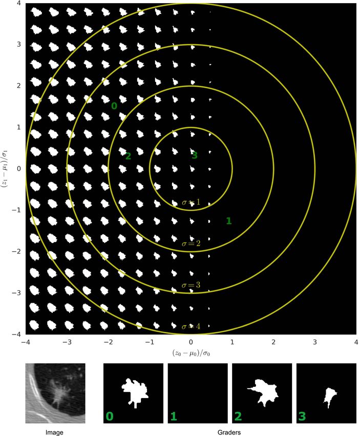
and sub-optimal treatment. Providing only pixel-wise probabilities ignores all co-variances between
the pixels, which makes a subsequent analysis much more difficult if not impossible. If multiple
consistent hypotheses are provided, these can be directly propagated into the next step in a diagnosis
pipeline, they can be used to suggest further diagnostic tests to resolve the ambiguities, or an expert
with access to additional information can select the appropriate one(s) for the subsequent steps.
Here we present a segmentation framework that provides multiple segmentation hypotheses for
ambiguous images (Fig. 1a). Our framework combines a conditional variational auto encoder (CVAE)
[2, 3, 4, 5] which can model complex distributions, with a U-Net [6] which delivers state-of-the-art
segmentations in many medical application domains. A low-dimensional latent space encodes the
possible segmentation variants. A random sample from this space is injected into the U-Net to
produce the corresponding segmentation map. One key feature of this architecture is the ability to
model the joint probability of all pixels in the segmentation map. This results in multiple segmentation
maps, where each of them provides a consistent interpretation of the whole image. Furthermore our
framework is able to also learn hypotheses that have a low probability and to predict them with the
corresponding frequency. We demonstrate these features on a lung abnormalities segmentation task,
where each lesion has been segmented independently by four experts, and on the Cityscapes dataset,
where we artificially flip labels with a certain frequency during training.
A body of work with different approaches towards probabilistic and multi-modal segmentation exists.
The most common approaches provide independent pixel-wise probabilities. E.g. probabilistic seg-
mentation methods that involve learning a posterior distribution over network weights or additionally
pixel-wise distributions over the network’s output have been proposed [7, 8]. These distributions
however treat pixels independently and individual samples therefore can not constitute valid hy-
potheses. A simple way to produce plausible hypotheses is to learn an ensemble of (deep) models
[9]. While the outputs produced by ensembles are consistent, they are not necessarily diverse and
ensembles are typically not able to learn the rare variants as their members are trained independently.
In order to overcome this, several approaches train models jointly using the oracle set loss [10], i.e.
a loss that only accounts for the closest prediction to the ground truth. This has been explored in
[11] and [1] using an ensemble of deep networks, and in [12] and [13] using one common deep
network with M heads. While multi-head approaches may have the capacity to capture a diverse set
of variants, they are not equipped to learn the occurrence frequencies of individual variants. Two
common disadvantages of both ensembles and M heads models are their ungraceful scaling to large
numbers of hypotheses, and their requirement of fixing the number of allowed hypotheses at training
time. Another set of approaches to produce multiple diverse solutions relies on graphical models,
such as junction chains [14], and more generally Markov Random Fields [15, 16, 17, 18]. While
many of the previous approaches are guaranteed to find the best diverse solutions, these are confined
to structured problems whose dependencies can be described by tractable graphical models.
The task of image-to-image translation [19] tackles a very similar problem: an under-constrained
domain transfer of images needs to be learned. Many of the recent approaches employ generative
adversarial networks (GANs) which are known to suffer from challenges such as ‘mode-collapse’ [20].
In an attempt to solve the mode-collapse problem, the ‘bicycleGAN’ [21] involves a component that
is similar in architecture to ours. In contrast to our proposed architecture, their model encompasses
a fixed prior distribution and during training their posterior distribution is only conditioned on the
output image. Very recent work on generating appearances given a shape encoding [22] also combines
a U-Net with a VAE, and was developed concurrently to ours. In contrast to our proposal, their
training requires an additional pretrained VGG-net that is employed as a reconstruction loss.
The main contributions of this work are: (1) Our framework provides consistent segmentation maps
instead of pixel-wise probabilities and can therefore give a joint likelihood of modes. (2) Our model
can induce arbitrarily complex output distributions including the occurrence of very rare modes,
and is able to learn calibrated probabilities of segmentation modes. (3) Sampling from our model
is computationally cheap. (4) In contrast to many existing applications of generative models that
can only be qualitatively evaluated, our application and datasets allow quantitative performance
evaluation including penalization of missing modes.

                                                   2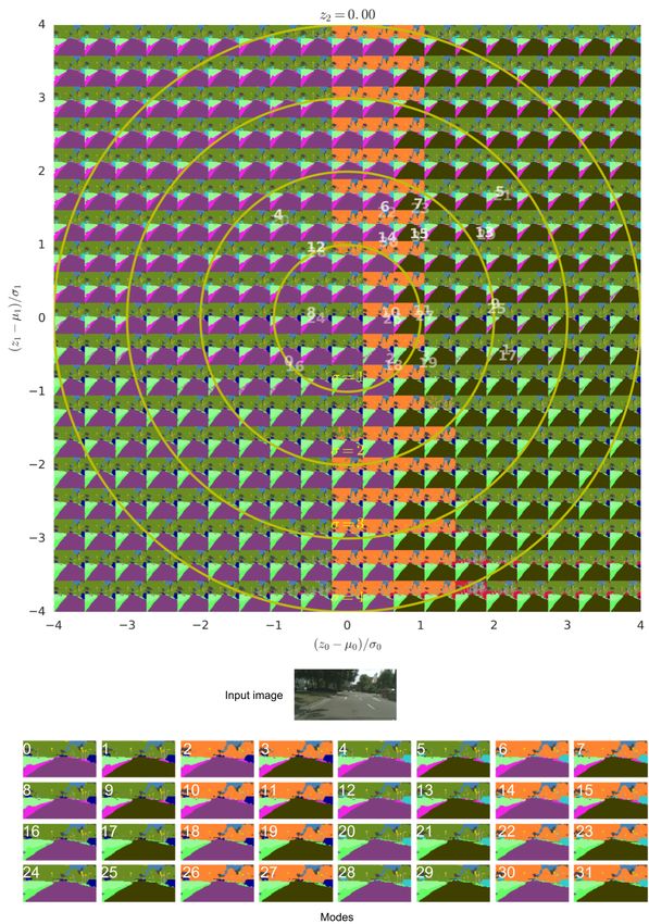
2 Network Architecture and Training Procedure
Our proposed network architecture is a combination of a conditional variational auto encoder [2, 3, 4]
with a U-Net [6], with the objective of learning a conditional density model over segmentations,
conditioned on the image.
a b
ᵤprior Posterior Net
ḙprior
z1 z2 ᵤpost,ḙpost
z3 ᵤprior
Prior Net ḙprior
Latent Space
1 z
Sample * KL
1,2,3,... Prior Net
Latent Space
2
Sample
Cross-
Entropy
Image 3
U-Net
Image Predicted Ground
Segmentation Truth
U-Net
Figure 1: The Probabilistic U-Net. (a) Sampling process. Arrows: flow of operations; blue blocks:
feature maps. The heatmap represents the probability distribution in the low-dimensional
latent space RN (e.g., N = 6 in our experiments). For each execution of the network,
one sample z ∈ RN is drawn to predict one segmentation mask. Green block: N -channel
feature map from broadcasting sample z. The number of feature map blocks shown is
reduced for clarity of presentation. (b) Training process illustrated for one training example.
Green arrows: loss functions.
Sampling. The central component of our architecture (Fig. 1a) is a low-dimensional latent space
RN (e.g., N = 6, which performed best in our experiments). Each position in this space encodes a
segmentation variant. The ‘prior net’, parametrized by weights ω, estimates the probability of these
variants for a given input image X. This prior probability distribution (called P in the following) is
modelled as an axis-aligned Gaussian with mean µprior (X; ω) ∈ RN and variance σ prior (X; ω) ∈ RN .
To predict a set of m segmentations we apply the network m times to the same input image (only
a small part of the network needs to be re-evaluated in each iteration, see below). In each iteration
i ∈ {1, . . . , m}, we draw a random sample zi ∈ RN from P
zi ∼ P (·|X) = N µprior (X; ω), diag(σ prior (X; ω)) , (1)
broadcast the sample to an N -channel feature map with the same shape as the segmentation map, and
concatenate this feature map to the last activation map of a U-Net (the U-Net is parameterized by
weights θ). A function fcomb. composed of three subsequent 1 × 1 convolutions (ψ being the set of
their weights) combines the information and maps it to the desired number of classes. The output, Si ,
is the segmentation map corresponding to point zi in the latent space:
Si = fcomb. fU-Net (X; θ), zi ; ψ . (2)
Notice that when drawing m samples for the same input image, we can reuse the output of the prior
net and the feature activations of the U-Net. Only the function fcomb. needs to be re-evaluated m
times.
Training. The networks are trained with the standard training procedure for conditional VAEs
(Fig. 1b), i.e. by minimizing the variational lower bound (Eq. 4). The main difference with respect to
training a deterministic segmentation model, is that the training process additionally needs to find a
useful embedding of the segmentation variants in the latent space. This is solved by introducing a
‘posterior net’, parametrized by weights ν, that learns to recognize a segmentation variant (given the
raw image X and the ground truth segmentation Y ) and to map this to a position µpost (X, Y ; ν) ∈ RN
with some uncertainty σ post (X, Y ; ν) ∈ RN in the latent space. The output is denoted as posterior
distribution Q. A sample z from this distribution,
z ∼ Q(·|X, Y ) = N µpost (X, Y ; ν), diag(σ post (X, Y ; ν)) , (3)
3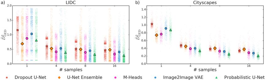
combined with the activation map of the U-Net (Eq. (1)) must result in a predicted segmentation S
identical to the ground truth segmentation Y provided in the training example. A cross-entropy loss
penalizes differences between S and Y (the cross-entropy loss arises from treating the output S as the
parameterization of a pixel-wise categorical
distribution
Pc ). Additionally there is a Kullback-Leibler
divergence KL(Q||P ) = Ez∼Q log Q − log P which penalizes differences between the posterior
distribution Q and the prior distribution P . Both losses are combined as a weighted sum with a
weighting factor β, as done in [23]:
h i
L(Y, X) = Ez∼Q(.|Y,X) − log Pc (Y |S(X, z)) + β · KL Q(z|Y, X)||P (z|X) . (4)
The training is done from scratch with randomly initialized weights. During training, this KL loss
“pulls” the posterior distribution (which encodes a segmentation variant) and the prior distribution
towards each other. On average (over multiple training examples) the prior distribution will be
modified in a way such that it “covers” the space of all presented segmentation variants for a specific
input image.
3 Performance Measures and Baseline Methods
In this section we first present the metric used to assess the performance of all approaches, and then
describe each competitor approach used in the comparisons.
As it is common in the semantic segmentation literature, we employ the intersection over union
(IoU) as a measure to compare a pair of segmentations. However, in the present case, we not only
want to compare a deterministic prediction with a unique ground truth, but rather we are interested
in comparing distributions of segmentations. To do so, we use the generalized energy distance
[24, 25, 26], which leverages distances between observations:
h i h 0
i h 0
i
2
DGED (Pgt , Pout ) = 2E d(S, Y ) − E d(S, S ) − E d(Y, Y ) , (5)
0
where d is a distance measure, Y and Y are independent samples from the ground truth distribution
0
Pgt , and similarly, S and S are independent samples from the predicted distribution Pout . The
energy distance DGED is a metric as long as d is also a metric [27]. In our case we choose d(x, y) =
1 − IoU(x, y), which as proved in [28, 29], is a metric. In practice, we only have access to samples
2
from the distributions that models induce, so we rely on statistics of Eq. (5), D̂GED . The details about
its computation for each experiment are presented in Sec. B in the Appendix.
With the aim of providing context for the performance of our proposed approach we compare against
a range of baselines. To the best of our knowledge there exists no other work that has considered
capturing a distribution over multi-modal segmentations and has measured the agreement with such
a distribution. For fair comparison, we train the baseline models whose architectures are depicted
in Fig. 2 in the exact same manner as we train ours. The baseline methods all involve the same
U-Net architecture, i.e. they share the same core component and thus employ comparable numbers of
learnable parameters in the segmentation tasks.
a b 1 c d Normal Prior
1
z1 z2
z3
2 2
Sample 1,2,3,...
1,2,3,...
m m
U-Net
Figure 2: Baseline architectures. Arrows: flow of operations; blue blocks: feature maps; red blocks:
feature maps with dropout; green block broadcasted latents. Note that the number of feature
map blocks shown is reduced for clarity of presentation. (a) Dropout U-Net. (b) U-Net
Ensemble. (c) M-Heads. (d) Image2Image VAE.
4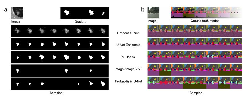
Dropout U-Net (Fig. 2a). Our ‘Dropout U-Net’ baselines follow the Bayesian segnet’s [7] proposi-
tion: we dropout the activations of the respective incoming layers of the three inner-most encoder
and decoder blocks with a dropout probability of p = 0.5 during training as well as when sampling.
U-Net Ensemble (Fig. 2b). We report results for ensembles with the number of members matching
the required number of samples (referred to as ‘U-Net Ensemble’). The original deterministic variant
of the U-Net is the 1-sample corner case of an ensemble.
M-Heads (Fig. 2c). Aiming for diverse semantic segmentation outputs, the works of [12] and [13]
propose to branch off M heads after the last layer of a deep net each of which contributes one output
variant. An adjusted cross-entropy loss that adaptively assigns heads to ground-truth hypotheses is
employed to promote diversity while reducing the risk of idle heads: the loss of the best performing
head is weighted with a factor of 1 − , while the remaining heads each contribute with a weight of
/(M − 1) to the loss. For our ‘M-Heads’ baselines we again employ a U-Net core and set  = 0.05
as proposed by [12]. In order to allow for the evaluation of 4, 8 and 16 samples, we train M-Heads
models with the corresponding number of heads.
Image2Image VAE (Fig. 2d). A U-Net VAE-GAN hybrid for multi-modal image-to-image trans-
lation, that owes its stochasticity to normal distributed latents that are broadcasted and fed into the
encoder path of the U-Net has been proposed in [21]. In order to deal with the complex solution
space in image-to-image translation tasks, they employ an adversarial discriminator as additional
supervision alongside a reconstruction loss. In the fully supervised setting of semantic segmentation
such an additional learning signal is however not necessary and we therefore train with a cross-entropy
loss only. In contrast to our proposition, this baseline, which we refer to as the ‘Image2Image VAE’,
employs a prior that is not conditioned on the input image (a fixed normal distribution) and a posterior
net that is not conditioned on the input either.
In all cases we examine the models’ performance when drawing a different number of samples (1, 4,
8 and 16) from each of them.

4     Results

A quantitative evaluation of multiple segmentation predictions per image requires annotations from
multiple labelers. Here we consider two datasets: The LIDC-IDRI dataset which contains 4 anno-
tations per input, and the Cityscapes dataset, which we artificially modify by adding synonymous
classes to introduce uncertainty in the way concepts are labelled.

4.1   Lung abnormalities segmentation

The LIDC-IDRI dataset [30, 31, 32] contains 1018 lung CT scans from 1010 lung patients with
manual lesion segmentations from four experts. This dataset is a good representation of the typical
ambiguities that appear in CT scans. For each scan, 4 radiologists (from a total of 12) provided
annotation masks for lesions that they independently detected and considered to be abnormal. We
use the masks resulting from a second reading in which the radiologists were shown the anonymized
annotations of the others and were allowed to make adjustments to their own masks.
For our experiments we split this dataset into a training set composed of 722 patients, a validation set
composed of 144 patients, and a test set composed of the remaining 144 patients. We then resampled
the CT scans to 0.5 mm × 0.5 mm in-plane resolution (the original resolution is between 0.461 mm
and 0.977 mm, 0.688 mm on average) and cropped 2D images (180 × 180 pixels) centered at the
lesion positions. The lesion positions are those where at least one of the experts segmented a lesion.
By cropping the scans, the resultant task is in isolation not directly clinically relevant. However, this
allows us to ignore the vast areas in which all labelers agree, in order to focus on those where there is
uncertainty. This resulted in 8882 images in the training set, 1996 images in the validation set and
1992 images in the test set. Because the experts can disagree whether the lesion is abnormal tissue,
up to 3 masks per image can be empty. Fig. 3a shows an example of such lesion-centered images and
the masks provided by 4 graders.
As all models share the same U-Net core component and for fairness and ease of comparability, we
let all models undergo the same training schedule, which is detailed in Sec. G.1 in the Appendix.

                                                   5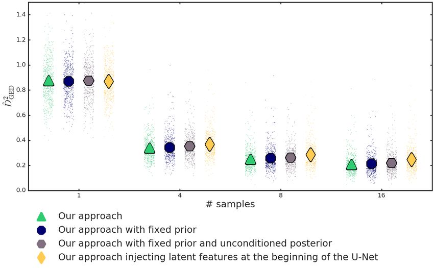
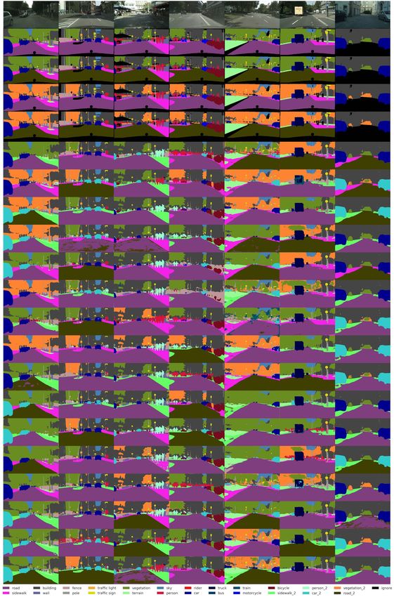
Figure 3: Qualitative results. The first row shows the input image and the ground truth segmentations.
          The following rows show results from the baselines and from our proposed method. (a)
          lung CT scan from the LIDC test set. Ground truth: 4 graders. (b) Cityscapes. Images
          cropped to squares for ease of presentation. Ground truth: 32 artificial modes. Best viewed
          in colour.

Figure 4: Comparison of approaches using the squared energy distance. Lower energy distances
          correspond to better agreement between predicted distributions and ground truth distribution
          of segmentations. The symbols that overlay the distributions of data points mark the mean
          performance. (a) Performance on lung abnormalities segmentation on our LIDC-IDRI
          test-set. (b) Performance on the official Cityscapes validation set (our test set).

In order to grasp some intuition about the kind of samples produced by each model, we show in Fig. 3a,
as well as in Sec. E in the Appendix, representative results for the baseline methods and our proposed
                                                                                 2
Probabilistic U-Net. Fig. 4a shows the squared generalized energy distance D̂GED    for all models as a
function of the number of samples. The data accumulations visible as horizontal stripes are owed
to the existence of empty ground-truth masks. The energy distance on the 1992 images large lung
abnormalities test set, decreases for all models as more samples are drawn indicating an improved
matching of the ground-truth distribution as well as enhanced sample diversity. Our proposed
Probabilistic U-Net outperforms all baselines when sampling 4, 8 and 16 times. The performance at
16 samples is found significantly higher than that of the baselines (p-value ∼ O(10−13 )), according
to the Wilcoxon signed-rank test.

4.2   Cityscapes semantic segmentation

As a second dataset we use the Cityscapes dataset [33]. It contains images of street scenes taken
from a car with corresponding semantic segmentation maps. A total of 19 different semantic classes
are labelled. Based on this dataset we designed a task that allows full control of the ambiguities:
we create ambiguities by artificial random flips of five classes to newly introduced classes. We flip
‘sidewalk’ to ‘sidewalk 2’ with a probability of 8/17, ‘person’ to ‘person 2’ with a probability of
7/17, ‘car’ to ‘car 2’ with 6/17, ‘vegetation’ to ‘vegetation 2’ with 5/17 and ‘road’ to ‘road 2’ with

                                                  6
probability 4/17. The choice of a prime denominator yields distinct probabilities for the ensuing
25 = 32 discrete modes. The official training dataset with fine-grained annotation labels comprises
2975 images and the validation dataset contains 500 images. We employ this offical validation set as
a test set to report results on, and split off 274 images (corresponding to the 3 cities of Darmstadt,
Mönchengladbach and Ulm) from the official training set as our internal validation set. As in the
previous experiment, in this task we use a similar setting for the training processes of all approaches,
which we present in detail in Sec. G.2 in the Appendix.
Fig. 3b shows samples of each approach in the comparison given one input image. In Sec. F in the
Appendix we show further samples of other images, produced by our approach. Fig. 4b shows that
the Probabilistic U-Net on the Cityscapes task outperforms the baseline methods when sampling 4, 8
and 16 times in terms of the energy distance. This edge in segmentation performance at 16 samples is
highly significant according to the Wilcoxon signed-rank test (p-value ∼ O(10−77 )). We have also
conducted ablation experiments in order to explore which elements of our architecture contribute to
its performance. These were (1) Fixing the prior, (2) Fixing the prior, and not using the context in the
posterior and (3) Injecting the latent features at the beginning of the U-Net. Each of these variations
resulted in a lower performance. Detailed results can be found in Sec. D in the Appendix.
Reproducing the segmentation probabilities. In the Cityscapes segmentation task, we can pro-
vide further analysis by leveraging our knowledge of the underlying conditional distribution that we
have set by design. In particular we compare the frequency with which every model predicts each
mode, to the corresponding ground truth probability of that mode. To compute the frequency of each
mode by each model, we draw 16 samples from that model for all images in the test set. Then we
count the number of those samples that have that mode as the closest (using 1-IoU as the distance
function).
0
Dropout U-Net U-Net Ensemble M-Heads Image2Image VAE Probabilistic U-Net
−1
−
log( )
P̂
2
−3
−∞
− 3 −2 − 1 0 −
3 −2 − 1 0 −
3 −2 − 1 0 −
3 −2 − 1 0 −
3 −2 − 1 0
P
log( ) P
log( ) P
log( ) P
log( ) P
log( )
Figure 5: Reproduction of the probabilities of the segmentation modes on the Cityscapes task. The
artificial flipping of 5 classes results in 32 modes with different ground truth probability
(x-axis). The y-axis shows the frequency of how often the model predicted this variant in
the whole test set. Agreement with the bisector line indicates calibration quality.
In Fig. 5 (and Figs. 8, 9, 10 in Appendix C) we report the mode-wise frequencies for all 32 modes
in the Cityscape task and show that the Probabilistic U-Net is the only model in this comparison
that is able to closely capture the frequencies of a large combinatorial space of hypotheses including
very rare modes, thus supplying calibrated likelihoods of modes. The Image2Image VAE is the only
model among competitors that picks up on all variants, but the frequencies are far off as can be seen
in its deviation from the bisector line in blue. The other baselines perform worse still in that all of
them fail to represent modes and the modes they do capture do not match the expected frequencies.
4.3 Analysis of the Latent Space
The embedding of the segmentation variants in a low-dimensional latent space allows a qualitative
analysis of the internal representation of our model. For a 2D or 3D latent space we can directly
visualize where the segmentation variants get assigned. See Appendix A for details.
5 Discussion and conclusions
Our first set of experiments demonstrates that our proposed architecture provides consistent segmen-
tation maps that closely match the multi-modal ground-truth distributions given by the expert graders
7in the lung abnormalities task and by the combinatorial ground-truth segmentation modes in the
Cityscapes task. The employed IoU-based energy distance measures whether the models’ individual
samples are both coherent as well as whether they are produced with the expected frequencies. It
not only penalizes predicted segmentation variants that are far away from the ground truth, but also
penalizes missing variants. On this task the Probabilistic U-Net is able to significantly outperform the
considered baselines, indicating its capability to model the joint likelihood of segmentation variants.
The second type of experiments demonstrates that our model scales to complex output distributions
including the occurrence of very rare modes. With 32 discrete modes of largely differing occurrence
likelihoods, the Cityscapes task requires the ability to closely match complex data distributions.
Here too our model performs best and picks the segmentation modes very close to the expected
frequencies, all the way into the regime of very unlikely modes, thus defying mode-collapse and
exhibiting excellent probability calibration. As an additional advantage our model scales to such large
numbers of modes without requiring any prior assumptions on the number of modes or hypotheses.
The lower performance of the baseline models relative to our proposition can be attributed to
design choices of these models. While the Dropout U-Net successfully models the pixel-wise data
distribution (Fig. 8 bottom right, in the Appendix), such pixel-wise mixtures of variants can not be
valid hypotheses in themselves (see Fig. 3). The U-Net Ensemble’s members are trained independently
and each of them can only learn the most likely segmentation variant as attested to by Fig. 8, top. In
contrast to that the closely related M-Heads model can pick up on multiple discrete segmentation
modes, due to the joint training procedure that enables diversity. The training does however not allow
to correctly represent frequencies and requires knowledge of the number of present variants (see
Fig. 9 top, in the Appendix). Furthermore neither the U-Net Ensemble, nor the M-Heads can deal
with the combinatorial explosion of segmentation variants when multiple aspects vary independently
of each other. The Image2Image VAE shares similarities with our model, but as its prior is fixed
and not conditioned on the input image, it can not learn to capture variant frequencies by allocating
corresponding probability mass to the respective latent space regions. Fig. 16 in the Appendix shows
a severe miss-calibration of variant likelihoods on the lung abnormalities task that is also reflected in
its corresponding energy distance. Furthermore, in this architecture, the latent samples are fed into
the U-Net’s encoder path, while we feed in the samples just after the decoder path. This design choice
in the Image2Image VAE requires the model to carry the latent information all the way through the
U-Net core, while simultaneously performing the recognition required for segmentation, which might
additionally complicate training (see analysis in Appendix D). Beside that, our design choice of late
injection has the additional advantage that we can produce a large set of samples for a given image at
a very low computational cost: for each new sample from the latent space only the network part after
the injection needs to be re-executed to produce the corresponding segmentation map.
Aside from the ability to capture arbitrary modes with their corresponding probability conditioned
on the input, our proposed Probabilistic U-Net allows to inspect its latent space. This is because
as opposed to e.g. GAN-based approaches, VAE-like models explicitly parametrize distributions,
a characteristic that grants direct access to the corresponding likelihood landscape. Appendix A
discusses how the Probabilistic U-Net chooses to structure its latent spaces.
Compared to aforementioned concurrent work for image-to-image tasks [22], our model disentangles
the prior and the segmentation net. This can be of particular relevance in medical imaging, where
processing 3D scans is common. In this case it is desirable to condition on the entire scan, while
retaining the possibility to process the scan tile by tile in order to be able to process large volumes
with large models with a limited amount of GPU memory.
On a more general note, we would like to remark that current image-to-image translation tasks only
allow subjective (and expensive) performance evaluations, as it is typically intractable to assess the
entire solution space. For this reason surrogate metrics such as the inception score based on the
evaluation via a separately trained deep net are employed [34]. The task of multi-modal semantic
segmentation, which we consider here, allows for a direct and thus perhaps more meaningful manner
of performance evaluation and could help guide the design of future generative architectures.
All in all we see a large field where our proposed Probabilistic U-Net can replace the currently applied
deterministic U-Nets. Especially in the medical domain, with its often ambiguous images and highly
critical decisions that depend on the correct interpretation of the image, our model’s segmentation
hypotheses and their likelihoods could 1) inform diagnosis/classification probabilities or 2) guide
steps to resolve ambiguities. Our method could prove useful beyond explicitly multi-modal tasks, as
8the inspectability of the Probabilistic U-Net’s latent space could yield insights for many segmentation
tasks that are currently treated as a uni-modal problem.
6 Acknowledgements
The authors would like to thank Mustafa Suleyman, Trevor Back and the whole DeepMind team for
their exceptional support, and Shakir Mohamed and Andrew Zisserman for very helpful comments
and discussions. The authors acknowledge the National Cancer Institute and the Foundation for
the National Institutes of Health, and their critical role in the creation of the free publicly available
LIDC/IDRI Database used in this study.
References
[1] Lee, S., Prakash, S.P.S., Cogswell, M., Ranjan, V., Crandall, D., Batra, D.: Stochastic multiple choice
learning for training diverse deep ensembles. In: Advances in Neural Information Processing Systems.
(2016) 2119–2127
[2] Kingma, D.P., Welling, M.: Auto-encoding variational bayes. In: Proceedings of the 2nd international
conference on Learning Representations (ICLR). (2013)
[3] Jimenez Rezende, D., Mohamed, S., Wierstra, D.: Stochastic backpropagation and approximate inference
in deep generative models. In: Proceedings of the 31st International Conference on Machine Learning
(ICML). (2014)
[4] Kingma, D.P., Jimenez Rezende, D., Mohamed, S., Welling, M.: Semi-supervised learning with deep
generative models. In: Neural Information Processing Systems (NIPS). (2014)
[5] Sohn, K., Lee, H., Yan, X.: Learning structured output representation using deep conditional generative
models. In: Advances in Neural Information Processing Systems. (2015) 3483–3491
[6] Ronneberger, O., Fischer, P., Brox, T.: U-net: Convolutional networks for biomedical image segmentation.
In: Medical Image Computing and Computer-Assisted Intervention (MICCAI) 2015. Volume 9351 of
LNCS., Springer (2015) 234–241
[7] Kendall, A., Badrinarayanan, V., Cipolla, R.: Bayesian segnet: Model uncertainty in deep convolutional
encoder-decoder architectures for scene understanding. arXiv preprint arXiv:1511.02680 (2015)
[8] Kendall, A., Gal, Y.: What uncertainties do we need in bayesian deep learning for computer vision? In:
Advances in Neural Information Processing Systems. (2017) 5580–5590
[9] Lakshminarayanan, B., Pritzel, A., Blundell, C.: Simple and scalable predictive uncertainty estimation
using deep ensembles. In: Advances in Neural Information Processing Systems. (2017) 6405–6416
[10] Guzman-Rivera, A., Batra, D., Kohli, P.: Multiple choice learning: Learning to produce multiple structured
outputs. In: Advances in Neural Information Processing Systems. (2012) 1799–1807
[11] Lee, S., Purushwalkam, S., Cogswell, M., Crandall, D., Batra, D.: Why m heads are better than one:
Training a diverse ensemble of deep networks. arXiv preprint arXiv:1511.06314 (2015)
[12] Rupprecht, C., Laina, I., DiPietro, R., Baust, M., Tombari, F., Navab, N., Hager, G.D.: Learning in an
uncertain world: Representing ambiguity through multiple hypotheses. In: International Conference on
Computer Vision (ICCV). (2017)
[13] Ilg, E., Çiçek, Ö., Galesso, S., Klein, A., Makansi, O., Hutter, F., Brox, T.: Uncertainty estimates for
optical flow with multi-hypotheses networks. arXiv preprint arXiv:1802.07095 (2018)
[14] Chen, C., Kolmogorov, V., Zhu, Y., Metaxas, D., Lampert, C.: Computing the m most probable modes of a
graphical model. In: Artificial Intelligence and Statistics. (2013) 161–169
[15] Batra, D., Yadollahpour, P., Guzman-Rivera, A., Shakhnarovich, G.: Diverse m-best solutions in markov
random fields. In: European Conference on Computer Vision, Springer (2012) 1–16
[16] Kirillov, A., Savchynskyy, B., Schlesinger, D., Vetrov, D., Rother, C.: Inferring m-best diverse labelings in
a single one. In: Proceedings of the IEEE International Conference on Computer Vision. (2015) 1814–1822
9[17] Kirillov, A., Shlezinger, D., Vetrov, D.P., Rother, C., Savchynskyy, B.: M-best-diverse labelings for
submodular energies and beyond. In: Advances in Neural Information Processing Systems. (2015)
613–621
[18] Kirillov, A., Shekhovtsov, A., Rother, C., Savchynskyy, B.: Joint m-best-diverse labelings as a parametric
submodular minimization. In: Advances in Neural Information Processing Systems. (2016) 334–342
[19] Isola, P., Zhu, J.Y., Zhou, T., Efros, A.A.: Image-to-image translation with conditional adversarial networks.
arXiv preprint (2017)
[20] Goodfellow, I.: Nips 2016 tutorial: Generative adversarial networks. arXiv preprint arXiv:1701.00160
(2016)
[21] Zhu, J.Y., Zhang, R., Pathak, D., Darrell, T., Efros, A.A., Wang, O., Shechtman, E.: Toward multimodal
image-to-image translation. In: Advances in Neural Information Processing Systems. (2017) 465–476
[22] Esser, P., Sutter, E., Ommer, B.: A variational u-net for conditional appearance and shape generation.
arXiv preprint arXiv:1804.04694 (2018)
[23] Higgins, I., Matthey, L., Pal, A., Burgess, C., Glorot, X., Botvinick, M., Mohamed, S., Lerchner, A.:
beta-vae: Learning basic visual concepts with a constrained variational framework. (2016)
[24] Bellemare, M.G., Danihelka, I., Dabney, W., Mohamed, S., Lakshminarayanan, B., Hoyer, S., Munos, R.:
The cramer distance as a solution to biased wasserstein gradients. arXiv preprint arXiv:1705.10743 (2017)
[25] Salimans, T., Zhang, H., Radford, A., Metaxas, D.: Improving gans using optimal transport. arXiv preprint
arXiv:1803.05573 (2018)
[26] Székely, G.J., Rizzo, M.L.: Energy statistics: A class of statistics based on distances. Journal of statistical
planning and inference 143(8) (2013) 1249–1272
[27] Klebanov, L.B., Beneš, V., Saxl, I.: N-distances and their applications. Charles University in Prague, the
Karolinum Press (2005)
[28] Kosub, S.: A note on the triangle inequality for the jaccard distance. arXiv preprint arXiv:1612.02696
(2016)
[29] Lipkus, A.H.: A proof of the triangle inequality for the tanimoto distance. Journal of Mathematical
Chemistry 26(1-3) (1999) 263–265
[30] Armato, I., Samuel, G., McLennan, G., Bidaut, L., McNitt-Gray, M.F., Meyer, C.R., Reeves, A.P., Clarke,
L.P.: Data from lidc-idri. the cancer imaging archive. http://doi.org/10.7937/K9/TCIA.2015.
LO9QL9SX (2015)
[31] Armato, S.G., McLennan, G., Bidaut, L., McNitt-Gray, M.F., Meyer, C.R., Reeves, A.P., Zhao, B., Aberle,
D.R., Henschke, C.I., Hoffman, E.A., et al.: The lung image database consortium (lidc) and image database
resource initiative (idri): a completed reference database of lung nodules on ct scans. Medical physics
38(2) (2011) 915–931
[32] Clark, K., Vendt, B., Smith, K., Freymann, J., Kirby, J., Koppel, P., Moore, S., Phillips, S., Maffitt, D.,
Pringle, M., et al.: The cancer imaging archive (tcia): maintaining and operating a public information
repository. Journal of digital imaging 26(6) (2013) 1045–1057
[33] Cordts, M., Omran, M., Ramos, S., Rehfeld, T., Enzweiler, M., Benenson, R., Franke, U., Roth, S., Schiele,
B.: The cityscapes dataset for semantic urban scene understanding. In: Proceedings of the IEEE conference
on computer vision and pattern recognition. (2016) 3213–3223
[34] Salimans, T., Goodfellow, I., Zaremba, W., Cheung, V., Radford, A., Chen, X.: Improved techniques for
training gans. In: Advances in Neural Information Processing Systems. (2016) 2234–2242
[35] Kingma, D.P., Ba, J.: Adam: A method for stochastic optimization. arXiv preprint arXiv:1412.6980 (2014)
10Appendix A Visualization of latent spaces
The segmentation variants from the proposed Probabilistic U-Net correspond to latent space samples from the
learned prior distribution. Fig. 6 and Fig. 7 below show samples from the Probabilistic U-Net for an LIDC-IDRI
and a Cityscapes example respectively. The samples are arranged so as to represent their corresponding position
in a 2D-plane of the respective latent space. This allows to interpret how the model ends up structuring the space
to solve the given tasks.
A.1 Lung Abnormalities Segmentation
In the LIDC-IDRI case the z0 -component of the prior happens to roughly encode lesion size including a
transition to complete lesion absence. The probability mass allocated to absence is relatively small in the
particular example, which arguably is in tune with the fact that 1 of the 4 graders assessed the image as lesion
free. The z1 -component on the other hand appears to encode shape variations. In the training, the posterior and
the prior distribution are tied by means of the KL-divergence. As a consequence they ‘live’ in the same space
and the graders (alongside the image to condition on) can be projected into the same latent space. Fig. 6 shows
the grader’s position in the form of green dots. The three graders that agree on presence, map into the 1-sigma
interval of the prior, while the grader predicting absence falls just short of the 4-sigma isoprobability contour in
the latent-space area that encodes absence. Fig. 3 gives more LIDC-IDRI examples with their corresponding
grader masks and 16 random samples of the Probabilistic U-Net. It appears that our model agrees very well
with cases for which there is inter-grader disagreement on lesion presence. For cases where the graders agree
on presence, our model at times apparently shows an under-conservative prior, in the sense that uncertainty
on presence can be elevated. The shape variations however are covered to a very good degree as attested by
quantitative experiments above.
A.2 Street Scene Segmentation
In the Cityscapes task we employ a latent space with more dimensions than on the lung abnormalities task in
order to equip the prior with sufficient capacity to encode the grader modes. The best performing model used
a 6D latent space, however, for ease of presentation the following discusses the latent structure of a 3D latent
space version. Fig. 7 shows a z0 -z1 plane of the latent space in which we again map corresponding segmentation
samples, this time for a Cityscapes example. The precisely defined grader modes in the Cityscapes task can be
identified with coherent regions in the latent space. As the space is 3D, not all 32 modes are fully manifest in the
shown z2 -slice. The location of the modes is shown via white mode numbers and the degree of transparency
indicated the proximity in z2 relative to the shown slice. As this particular task involves discrete modes, the
semantically different regions are coherent and well confined as hoped for. There however inevitably are
transitions between those latent space regions that will translate to mixtures of the grader modes that cross over.
Ideally these transitions are as sharp as possible relative to the order of magnitude of the prior variance, which is
arguably the case. Fig. 17 shows Cityscapes examples with their corresponding grader masks and 16 random
samples of the Probabilistic U-Net. The shown samples exhibit largely coherent variants alongside occasional
variant mixtures that correspond to semantic cross overs in the latent space. As alluded to quantitatively before,
the samples also appear to respect the grader variant frequencies, which are captured by structuring the latent-
space under the prior in such fashion that the correct probability mass is allocated to the respective mode. In
the upper boundary region of Fig. 7 improper samples are found that show miss-segmentations (although those
are unlikely under the prior). The erroneously encoded modes found here are presumably attributable to the
presence of inherent ambiguities in the dataset.
Appendix B Metrics
In the LIDC dataset, given that we have m = 4 ground truth samples and n samples from the models, we employ
the following statistic:
n m n n m m
2 2 XX 1 XX 0 1 XX 0
D̂GED (Pgt , Pout ) = d(Si , Yj ) − 2 d(Si , Sj ) − 2 d(Yi , Yj ). (6)
nm i=1 j=1 n i=1 j=1 m i=1 j=1
In the case that both arguments of the distance function have empty lesion masks, we define its distance to be 0,
so that the metric rewards the agreement on lesion absence.
On the Cityscapes task, given that we have defined the settings, we have full knowledge about the ground truth
distribution, which is a mixture of M = 32 Dirac delta distributions. Hence, we do not need to sample from it,
but use it directly in the estimator:
n M n n M X M
2 2 XX 1 XX 0 X 0
D̂GED (Pgt , Pout ) = d(Si , Yj )ωj − 2 d(Si , Sj ) − d(Yi , Yj )ωi ωj , (7)
n i=1 j=1 n i=1 j=1 i=1 j=1
11where ωj is the weight for the j-th mixture, which is a delta distribution containing all the density in Yj .
Appendix C How models fit the ground truth distribution
In this section we analyse the frequency in which each mode of the Cityscape task is targeted by each model,
and how much that varies from the ground truth distribution. We report the mode-wise and pixel-wise marginal
occurrence frequencies of the sampled segmentation variants. In the mode-wise case, each sample is matched
to its closest ground truth mode (using 1-IoU as the distance function). Then, the frequency of each mode
is computed by counting the number of samples that most closely match that mode. In the pixel-wise case,
the marginal frequencies p(predicted class|ground-truth class) are obtained by counting all pixels across all
images and corresponding samples that show a valid pixel hypothesis given the ground-truth, normalized by the
number of respective uni-modal ground-truth pixels. In Fig. 8 we present the results for U-Net Ensemble and
Dropout U-Net, in Fig. 9 we show the results for M-Heads and Image2Image VAE, finally in Fig. 10 we present
the results for our approach.
Appendix D Ablation analysis
In this section we explore variations in the architecture of our approach, in order to understand how each design
decision affects the performance. We have tried three variations over the original approach, these are:
Fixing the prior: Instead of making the prior a function of the context, here we fix it to be a standard Gaussian
distribution.
Fixing the prior, and not using the context in the posterior: In addition to fixing the prior to be Gaussian, we
also make the posterior a function of the ground truth mask only, ignoring the context.
Injecting the latent features at the beginning of the U-Net: Starting from our original model, we change the
position in which the latent variables are used. Specifically here we concatenate them to the context (input
image) and propagate that through the U-Net.
In Fig 11 we can observe that our approach is better than the other variations. As the mechanisms that induce
the distributions over segmentations during sampling and training are blinded towards the context image, the
performance in terms of the IoU-based energy distance decreases. In particular, our model is much better than
the variation that injects latent samples at the beginning. This is a pleasant finding, given that our decision
of injecting the latent variables at the end of the U-Net was motivated by efficiency reasons when sampling.
Here we find that we do not lose performance by doing so, but instead observe an improved matching of the
samples with the ground-truth distribution. We hypothesize that injecting the latent variables at the final stage
of the pipeline makes it easier for the model to account for different segmentations given the same input. This
hypothesis is supported by the slightly better performance shown by the alternative architecture when sampling
only once, and how this advantage is lost, and actually reversed, when sampling several times.
Appendix E Sampling LIDC masks using different models
Fig. 12-16 show samples of our proposed model as well as all the baselines given the same input images. For
reference the expert segmentations are shown in the four rows just below the images.
Appendix F Sampling Cityscapes segmentations using our model
Fig. 17 shows samples of our proposed model on the Cityscapes dataset, and Table 1 shows the numerical results
from Fig. 4 (b), so that new approaches can be compared to those.
# Samples 1 4 8 16
2
D̂GED 0.874 0.337 0.248 0.206
Table 1: Numerical (mean) results of the Probabilistic U-Net on Cityscapes, taken from Fig. 4 (b).
Appendix G Training details
In this section we describe the architecture settings and training procedure for both experiments.
12G.1 Lung abnormalities segmentation
During training image-grader pairs are drawn randomly. We apply augmentations to the image tiles (180 × 180
pixels size): random elastic deformation, rotation, shearing, scaling and a randomly translated crop that results
in a tile size of 128 × 128 pixels. The U-Net architecture we use is similar to [6] with the exception that we
down- and up-sample feature maps by using bilinear interpolations. The cores of all models are identical and
feature 4 down- and up-sampling operations, at each scale the blocks comprise three convolutional layers with
3 × 3-kernels, each followed by a ReLU-activation. In our model, both the prior and the posterior (as well
as the posterior in Image2Image VAE) nets have the same architecture as the U-Net’s encoder path, i.e. they
are made up to the same number of blocks and type of operations. Their last feature maps are global average
pooled and fed into a 1 × 1 convolution that predicts the Gaussian distributions parameterized by mean and
standard deviation. The architecture last layers, corresponding to fcomb. , comprise the appropriate number of
1 × 1-kernels and are activated with a softmax. The base number of channels is 32 and is doubled or respectively
halved at each down- or up-sampling transition. All individual models share this core component and for ease of
comparability we let all models undergo the same training schedule: the training proceeds over 240 k iterations
with an initial learning rate of 1e−4 that is lowered to 1e−6 in 5 steps. All weights of all models are initialized
with orthogonal initialization having the gain (multiplicative factor) set to 1, and the bias terms are initialized by
sampling from a truncated normal with σ = 0.001. We use a batch-size of 32, weight-decay with weight 1e−5
and optimize using the Adam optimizer with default settings [35]. A KL weight of β = 10 with a latent space of
3 dimensions gave best validation results for the baseline Image2Image VAE, and β = 1 and a 6D latent space
performed well for the Probabilistic U-Net, although the performances were alike across the hyperparameters
tried on the validation set.
G.2 Cityscapes
We down-sample the Cityscapes images and label maps to a size of 256 × 512. Similarly to above, we apply
random elastic deformation, rotation, shearing, scaling, random translation and additionally impose random color
augmentations on the images during training. The U-Net cores in this task are identical to the ones above, but
process an additional feature scale (implying one additional up- and one additional down-sampling operation).
The training procedure is also equivalent to the previous experiment, also using 240 k iterations, except that
here we employ a batch-size of 16, and the initial learning rate of 1e−4 is lowered to 0.5e−6 in 4 steps. The
Cityscapes dataset includes ignore label masks for each image with which we mask the loss during training,
and the metric during evaluation. A KL weight of β = 1 and 3D latents gave best validation results for the
Image2Image VAE and a β = 1 and 6D latents performed best for the Probabilistic U-Net (although 3-5D
performed similarly).
13Figure 6: Visualization of the latent space for the lung abnormalities segmentation. 19 × 19 samples
for a LIDC-IDRI test set example mapped to their prior latent-space position, using our
model trained with a latent space of only 2 dimensions. For ease of presentation, the latent
space is re-scaled so that the prior likelihood is a spherical unit-Gaussian. The isoprobable
yellow circles denote deviations from the mean in sigma. The ground-truth grader masks’
posterior position in this latent space is indicated by green numbers. The input image is
shown in the lower left, to the right of it, the 4 grader masks are shown.
14Figure 7: Visualization of the latent space for the Cityscapes task. 19 × 19 samples of a Cityscapes
validation set example, mapped here to their latent-space position in the z0 -z1 plane (z2 = 0)
of the learned prior, using our model trained with a latent space of only 3 dimensions.
For ease of presentation, the samples are squeezed to rectangles and the latent space is
re-scaled so that the prior likelihood is a spherical unit-Gaussian. The isoprobable yellow
circles denote deviations from the mean in sigma. The ground-truth grader masks’ posterior
position in this latent space is indicated by white numbers. (color-map as in Fig 17).
15Figure 8: Reproduction of probabilities by the baselines Dropout U-Net and U-Net Ensemble. The
vertical histogram shows the mode-wise occurrence frequencies of samples in comparison
to the ground-truth probability of the modes, and the horizontal histogram reports the
pixel-wise marginal frequencies, i.e. the sampled pixel-fractions for each new stochastic
class (e.g. sidewalk 2) with respect to the corresponding existing one (sidewalk).
16Figure 9: Reproduction of probabilities by the baselines M-Heads and Image2Image VAE. The
vertical histogram shows the mode-wise occurrence frequencies of samples in comparison
to the ground-truth probability of the modes, and the horizontal histogram reports the
pixel-wise marginal frequencies, i.e. the sampled pixel-fractions for each new stochastic
class (e.g. sidewalk 2) with respect to the corresponding existing one (sidewalk)
17Figure 10: Reproduction of probabilities by our Probabilistic U-Net.The vertical histogram shows
the mode-wise occurrence frequencies of samples in comparison to the ground-truth
probability of the modes, and the horizontal histogram reports the pixel-wise marginal
frequencies, i.e. the sampled pixel-fractions for each new stochastic class (e.g. sidewalk
2) with respect to the corresponding existing one (sidewalk).
Figure 11: Ablation analysis. Comparison of architectural variations of our approach using the energy
distance. Lower energy distances correspond to better agreement between predicted
distributions and ground truth distribution of segmentations. The symbols that overlay the
distributions of data points mark the mean performance.
18c U-Net
graders
samples
Figure 12: Qualitative examples from the Probabilistic U-Net. The upper panel shows LIDC test
set images from 15 different subjects alongside the respective ground-truth masks by the
4 graders. The panel below gives the corresponding 16 random samples from the network.
19Figure 13: Qualitative examples from the Dropout U-Net. Same layout as Fig. 12.
20Figure 14: Qualitative examples from the U-Net Ensemble. Same layout as Fig. 12.
21Figure 15: Qualitative examples from the M-Heads (using a network with 16 heads). Same layout as
Fig. 12.
22e VAE
3 graders
samples
Figure 16: Qualitative examples from the Image2Image VAE. Same layout as Fig. 12.
23Figure 17: Qualitative examples from the Probabilistic U-Net on the Cityscapes task. The first row
shows Cityscapes images, the following 4 rows show 4 out of the 32 ground truth modes
with black pixels denoting pixels that are masked during evaluation. The remaining 16
rows show random samples of the network.
24You can also read