Space-Based Spooky Radar Orbit Determination Benefits at Earth-Moon Lagrange Points Darin C. Koblick and Steven Wilkinson
←
→
Page content transcription
If your browser does not render page correctly, please read the page content below
Space-Based Spooky Radar Orbit Determination Benefits at Earth-Moon Lagrange Points

                                Darin C. Koblick and Steven Wilkinson
                         Raytheon Intelligence and Space, El Segundo, 90245, USA

                                                         ABSTRACT

We present a cislunar metric tracking performance analysis using the range and angle measurements offered by a
quantum entangled-photon radar, otherwise known as a “Spooky Radar”, from Lissajous orbits around L1, L4 and
L5 Earth-Moon Lagrange points. There are five known Earth-Moon Lagrange points where a satellite/observer can
maintain a relative periodic trajectory - often described as a Lissajous orbit. A Space Based Spooky Radar located at
one of these orbital positions would be particularly effective since they are stable and have a combined field of regard
which is never simultaneously eclipsed by either Earth-Moon body, and maintain an unobstructed line-of-site with the
other Lagrange points.

Space Based Spooky Radars, coupled with traditional ground based optical and Radar measurements, are simulated
in tandem to estimate the orbit of a representative satellite in Geosynchronous Earth Orbit. A tracking scenario
was developed to quantify the relative performance improvement of state estimates over a traditional ground-based
sensor architecture mix. Results were computed using an Unscented Kalman Filter and underlying high-fidelity force
models. An introduction of slight solar radiation pressure drag and gravity gradient mismatching between the internal
filter state dynamics and the orbital propagator for a more accurate solution. Our analysis shows an order of magnitude
improvement in both position and velocity state estimates over conventional optical and radar systems.

                                                   1.   INTRODUCTION

Quantum entanglement and teleportation is driving the emerging technology revolution in computing, cryptography,
communications, and sensing. In 2016, the first quantum-encrypted video call was made possible with a quantum com-
munication satellite used to distribute a quantum key to separate geographical locations. In 2019, the first-ever photo
of quantum entanglement was revealed, several months later, quantum teleportation was used to send data between
two computer chips without physical or electrical connections. As of writing this article, physicists at the Institute
of Science and Technology Austria built the first working radar prototype exploiting quantum entanglement to detect
objects [1]. While much of this revolution is improving the efficiency of communications and computing on Earth,
the future performance advantages of using quantum technology for space applications have yet to be conceptualized.
This study is a first order performance assessment at the system level to understand the potential performance advan-
tages gained from using quantum remote sensing technology to assist with the space object metric tracking problem.

Quantum sensor technology has benefited significantly from advances in quantum information science. Proposed
quantum sensing technology applications include magnetometers, photodetectors, lasers, and gravitometers [2]. Ex-
amples of ongoing research include: the collaboration between Louisiana State University and Raytheon involving
quantum LiDAR remote sensing technologies [3], researchers at Caltech and MIT developing quantum enhanced
gravitational wave detectors [4], scientists at the University of Tokyo demonstrating an entanglement based detector
prototype [5], and engineers at Lockheed Martin have filed several patents describing a sensor systems using entangled
quantum particles [6].

An Entangled-Photon Quantum Radar (QR), also known as a “Spooky Radar”, exploits the quantum phenomena of
entanglement to gain detection supersensitivity and achieve super resolution performance in both range and angle mea-
surements. The absence of atmospheric attenuation for space-to-space (sat2 ) object tracking enables Quantum Radar
to achieve superior detection sensitivity over more traditional technology [7]. Range errors in Radar measurements

          Copyright © 2020 Advanced Maui Optical and Space Surveillance Technologies Conference (AMOS) – www.amostech.com
√
have a lower bound approaching the shot noise limit, δ R ≤ O(1/ N) , while Quantum Radar measurements exploit
quantum entanglement to quadratically lower this bound to the Heisenberg limit (e.g. super-resolution), such that
δ R ≤ O(1/N). These characteristics make quantum radar applications ideal for satellite orbit determination missions,
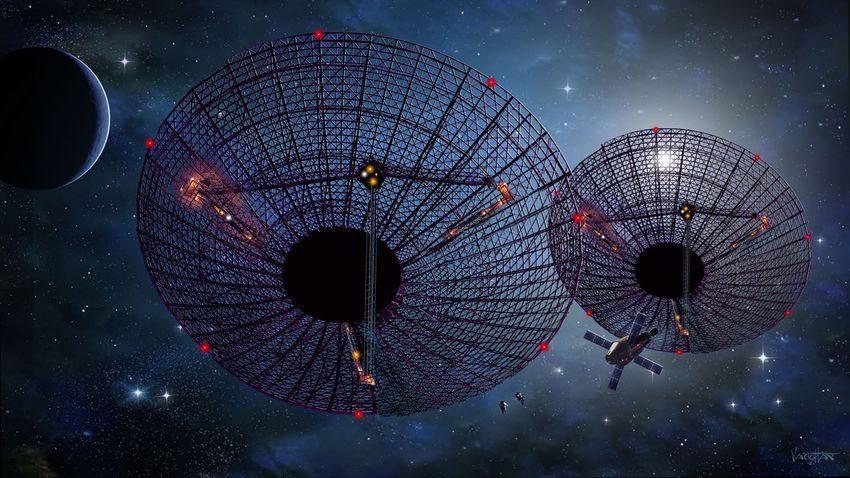
especially in conjunction with observation points much farther away than traditional space surveillance missions. Fig-
ure 1 is a concept illustration of a 25m diameter VHF homodyne quantum radar system at the Earth-Moon Lagrange
Point, L1 , sized to detect 1m diameter objects at ranges of over 400,000 km.
Fig. 1: Concept Illustration of a Quantum Radar at the L1 Earth-Moon Lagrange Point courtesy of James Vaughan at
http://www.jamesvaughanphoto.com/
Cislunar space, the region between low Earth orbit and the moon, has become increasingly crowded and competitive.
Agencies such as the US Space Force are seeking to extend their space situational awareness capabilities to include
cislunar space during peacetime and conflict [8]. The current Space Surveillance Network (SSN) employs Ground-
based Electro-Optical Deep Space Surveillance (GEODSS) optical systems to track objects from 4,800 to 56,000 km
in altitude [9]. While GEODSS may track satellites greater than the size of a chair at Molniya altitudes [9], it provides
angles-only measurements which require fusion from other sensors to provide a full three dimensional state estimate.
GEODSS can only operate during nighttime, so there’s 12-17 hours of downtime between tracks [10]. Figure 1 de-
picts a geosynchronous orbit (red circle), the GEODSS maximum range (green circle), and three Earth-Moon lagrange
points. If high sensitivity quantum radar systems were put on L1 , L4 , and L5 with an effective range of 400,000 km,
near persistent simultaneous tracking coverage of objects from low earth orbits to GEO, and the entire corridor be-
tween Earth and L2 would be possible (blue outline).
Copyright © 2020 Advanced Maui Optical and Space Surveillance Technologies Conference (AMOS) – www.amostech.comFig. 2: Quantum Radar Field of Regard from Earth-Moon Lagrange Points L1 , L4 , and L5
2. N00N STATE QUANTUM INTERFEROMETRY
Entanglement is a highly attractive feature for engineers and scientists utilizing quantum technology. Multi-particle
entangled states, core to many technologies exploiting quantum mechanics, can improve precision in phase measure-
ments. One useful subset of entanglement is the multiphoton entangled states otherwise known as “N00N” states, a
quantum-mechanical many-body entangled state described as
|Nia |0ib + eiNφ |0ia |Nib
|ψN00N i = √ , (1)
2
representing the superposition of N photons in mode a with zero (0) photons in mode b with zero (0) photons in mode
a with N photons in mode b, which represents a “N00N” sequence [11]. The phase, φ , can be estimated by measuring
an observable given by
A = |N, 0ih0, N| + |0, NihN, 0| (2)
where the N00N state switches between +1 and -1 as the phase alternates from 0 to π/N. Under lossless conditions
(e.g. vacuum of space), the phase measurement error approaches the Heisenberg limit via [12]
∆A 1
∆φ = = (3)
dhAi/dφ N
Knowing the phase measurement error, N00N states with N entangled photons can acquire a phase N times faster than
classical light [13] leading to enhanced phase sensitivity and super-resolution allowing quantum sensing systems to
surpass the diffraction limit (e.g. φ = 1.22λ /D).
3. SPHERICAL RADAR CROSS SECTION ESTIMATION
The classical radar cross section (RCS) of a perfect sphere can be determined analytically, for a spherical radius, a, the
RCS is calculated based on the Rayleigh scattering (λ >> a ) and optical limits (λFor spherical targets, there exists an analytical expression for the Quantum Radar Cross Section (QRCS), identical to
the classical RCS, such that [2]
σQ = σ . (5)
4. RANGE MEASUREMENT ACCURACY
For conventional pulse radar systems, the accuracy of a given range measurement is dominated by the Signal-to-Noise
Ratio (SNR) of the system and its pulse width τ. The standard deviation is a function of the range resolution, ∆R, via
[17]
c 1
σR = ·√ (6)
2∆ω 2 · SNR
where c is the speed of light, ∆ω is the bandwidth (e.g. 1/τ) of the transmitted pulse, SNR is the signal-to-noise ratio
of the target, and the radar range resolution, ∆R = c/2∆ω.
The use of quantum entangled photon measurements can exploit the super sensitivity phenomenon. Super sensitivity
commonly describes measurement errors less than the shot noise limit, and in the case of space-based N00N state
quantum radars, will exceed the quantum limit and approach the Heisenberg limit [18].
Measurements in classical quantum mechanics obey the Heisenberg uncertainty principle via
σφ σN = ∆φ ∆N ≥ 1 (7)
where ∆φ and ∆N are the phase and photon number uncertainties respectively. Assuming a monochromatic coherent
state, the probability of finding p
N photons comes in the form of a Poisson distribution which
√ allows us to compute
the standard deviation as σN = hNi and, using the inequality in Equation 7, σφ = 1/ N. Measuring the relative
distance, ∆R, between objects with phase measurements depends upon the wavelength and phasing via [19]
∆R
φ = 2π . (8)
λ
Using standard deviations, Equation 8 can also describe the range accuracy performance of a quantum interferometer
λ
σR ≈ · σφ . (9)
2π
If there’s a specific value on the fluctuation in photon count, the standard quantum limit could be avoided using optimal
measurement strategies (e.g. N00N state) such that σN2 = hNi2 , approaches the Heisenberg limit, σφ = 1/N. Thus, for
photonic interferometry there are two minimum range measurement error bounds approximated by
√
λ 1/ N, Shot Noise Limit (Non-Entangled Quantum Interferometry)
σRQ ≈ · (10)
2π 1/N, Heisenberg Limit (N00N Entangled State Quantum Interferometry)
5. ANGLE MEASUREMENT ACCURACY
Although not a requirement for precision orbit determination, having both angle and range measurements can signifi-
cantly reduce state estimation errors and the number of observers required to maintain “observability”. Consider two
apertures separated by length, L, and connected via waveguides to a beam splitter. The received signal photons, now
split between two apertures,√will have a relative phase shift resulting the physical separation between them. The phase
resolution follows ∆φ = 1/ N when the signal plane wave angle, Θ, is zero. Since the separation distance between
the two apertures is known, a super resolved measurement of both the azimuthal and altitudinal angles can be made in
accordance with [20]
λ 1
σΘQ = √ . (11)
2πL N
Copyright © 2020 Advanced Maui Optical and Space Surveillance Technologies Conference (AMOS) – www.amostech.comwhere λ is the wavelength of the quantum radar frequency and N is the number of signal photons.
The angular resolution is proportional to the 3-dB beam width (i.e. half-power beam width), θ3dB , for conventional
radar systems. The theoretical performance of a monopulse radar is included for reference as [21]
θ3dB
σΘ = √ . (12)
2 · SNR
where the half-power beam width for a typical parabolic antenna of diameter, D, and center wavelength, λ , is estimated
from [22]
1.2217λ
θ3dB = . (13)
D
6. DETECTION SENSITIVITY
Signal-to-Noise (SNR) is defined as the square of ratio of the signal mean, Ns , to the standard deviation of noise,σn ,
such that
Ns PR
SNR = = , (14)
σn NEP
noting that the above definition is also equivalent to using the effective received power, PR , and the noise equivalent
power (NEP). For low noise environments, such as space-to-space object detection, all noise source contributions,
other than shot noise, approach zero and NEP will approach the shot noise limit of the sensor, NEP → ησ . For a
monostatic quantum radar, the effective received power from a spherical target is obtained from the “quantum radar
equation” [2],
Pt Ar σ Q
PRQ = , (15)
(4π)2 R4
where R is the range to the target, Ar , is the aperture area of the receiver, and Pt is the transmitted power. The SNR
determined from the standard quantum limit (SQL), SNR, [23] is
!1/2
ηPRQ
SNR = , (16)
hν∆ν
where η is the quantum efficiency of the detector, h is Planck’s constant, ν is the frequency of the incident photons,
and ∆ν is the frequency interval over which the fluctuations are integrated.
7. PROBABILITY OF DETECTION
Two separate algorithms are presented to compute the probability of a sensor system to detect an object. The first
algorithm deals with very low photon counts where both the number of received signal photons, Ns , and the number of
noise photons, Nnoise , is less than unity. The second algorithm is commonly applied when there are many signal and
noise photons received over an integration period and Gaussian statistics is applicable.
7.1 Quantum Illumination Pd Algorithm (SNR ≤ 1)
Suppose a single stream of photons is sent through space via electromagnetic wave to detect the reflected photons
from a target near the maximum range limit of the system. In this case, the number of photons received is very small
(Ns < 1). There are two types of received photons at any given instant in time, those reflected from the target (e.g.
signal), and those resulting from quantum shot noise as computed from the “Quantum Shot Noise Limit” (e.g. noise)
, used to determine the maximum SNR in Equation 16
s
∆νNs
Nnoise = . (17)
η
Copyright © 2020 Advanced Maui Optical and Space Surveillance Technologies Conference (AMOS) – www.amostech.comEquation 17 is derived from knowing that the number of photons received per second (photon flux) is found from
Planck’s law [24]
P
Φ= . (18)
hν
The integration time, tint , of the system is selected to ensure that both signal photons received and noise photons are
less than or equal to unity, that is,
Ns = Φs · tint ≤ 1 (19)
Nnoise = Φnoise · tint ≤ 1. (20)
Notice that the integration time is used to scale both noise and the signal to unity within a detection window, looking
at Equation 17, its easy to verify the SNR will remain constant when the number of signal and noise photons are
increased proportionally through longer integration intervals (e.g. SNR = constant when tint > 0).
There are four conditional probabilities for target detection outcomes summarized below:
1. Noise Detected, Target Outside of Range (P(+|−) ): The probability that a noise photon is detected in the
absence of a signal photon is simply Nnoise .
2. Nothing Detected, Target Outside of Range (P(−|−) ): The probability that the target is not detected by the
system, and it’s also outside of the range limit suggests that no noise photons have been detected, the probability
of not detecting a noise photon is 1 − Nnoise .
3. Nothing Detected, Target Within Range (P(−|+) ): The probability that both the noise and the signal photon
are not detected is found from (1 − Nnoise ) · (1 − Ns )
4. Something Detected, Target Within Range (P(+|+) ): The probability that something is detected is found from
unity minus the probability that nothing is detected, 1 − P(−|+) .
Assuming that the photons sent toward the target are entangled, the effective noise is reduced to Nn /d where d is the
number of entangled modes [25]. The number of entangled modes, in terms of the number of e-bits of entanglement,
e, may be expressed as
d = 2e . (21)
Therefore, the conditional probabilities may be represented in terms of entanglement, Pe , and no entanglement, P in
Table 7.1
Outcome Symbol P([.]|[.]) Pe([.]|[.])
Detection, Outside Range (+|−) Nnoise Nnoise /d
No Detection, Outside Range (−|−) 1 − Nnoise 1 − Nnoise /d
No Detection, Within Range (−|+) (1 − Nnoise ) · (1 − Ns ) (1 − Nnoise /d) · (1 − Ns )
Detection, Within Range (+|+) 1 − (1 − Nnoise ) · (1 − Ns ) 1 − (1 − Nnoise /d) · (1 − Ns )
Table 1: Conditional Probabilities of Detection with vs without Entanglement, P, vs Pe .
The probability of false alarm, Pf a , is the probability that noise is detected in the absence of the target within range
P(+|−)
Pf a = e (22)
P(+|−)
The probability of detection, Pd , is defined as the probability that either noise or signal is detected in the presence of a
target within range
P(+|+)
Pd = e (23)
P(+|+)
Copyright © 2020 Advanced Maui Optical and Space Surveillance Technologies Conference (AMOS) – www.amostech.comThe ability to reduce the noise signal by increasing the number of entangled modes is extraordinary as it decreases the
probability of false alarms when the noise is greater than the signal (e.g. SNR < 1). A conditional probability model
is used in conjunction with the detection window probabilities to determine the overall probability of detection and
false alarm for longer integration intervals
Pd (n) = (P(+|+) )ncoadd (24)
Pf a (n) = 1 − (1 − P(+|−) )ncoadd , (25)
where ncoadd = t/tint . The total number of signal photons received over the longer integration time summed together
for an improvement in system range and angle accuracy via Equations 10 and 11, keep in mind this enhancement is
intended for targets which have insignificant relative motion over the full integration interval.
7.2 Classic Pd Algorithm (SNR > 1)
Assuming a signal shot noise limited environment (e.g. absence of additional noise sources outside of shot noise), the
probability of detection can be expressed int terms of SNR and Threshold to Noise Ratio (TNR) as [26][27][28]
1 SNR − T NR
Pd = 1 + er f √ , (26)
2 2
where TNR is computed directly from the Probability of False Alarm,
q √
T NR = −2ln( 3Pf a ). (27)
This can be applied to Radar and Optical sensors with Gaussian background noise, no atmospheric turbulence, and
higher SNR values (e.g. SNR > 1).
8. FILTER IMPLEMENTATION AND DYNAMICS MODEL
Many astrodynamic tracking problems have underlying dynamics and measurement processes that are nonlinear. A
logical step would be to extend the Kalman filter, (e.g. “Extended Kalman Filter”), however, an extended Kalman filter
requires Jacobian matrices such that the transformation from filter state to measurement can be applied, and calcula-
tions of the Jacobian and Hessian matrices are extremely difficult or prone to human error. The simulation and subse-
quent results in this paper utilize a nonaugmented unscented kalman filter (UKF) in conjunction with a high precision
orbit propagator and filter dynamics model via patent pending c code dynamic-link library called hyperTRAC™[29].
The UKF implemented in hyperTRAC™employs an unscented transform (UT) to provide a Gaussian approximation
to the filtering solutions of non-linear optimal filtering problems of the form:
Xk = f(xk−1 , k − 1) + Qk−1 (28)
Yk = h(xk , k) + rk (29)
where Xk ∈ IRn is the filter state estimate, Yk ∈ IRm is the measurement, Qk−1 ∼ N(0, Qk−1 ) is the Gaussian process
noise, and rk ∼ N(0, Rk ) is the Gaussian measurement noise. f(.) represents the non-linear function which propagates
the state with respect to time, h(.) represents a non-linear transformation function which converts the current state to
measurements relative to a specific observer [30].
8.1 Measurement Model
Assume an observer can measure range, azimuth, and elevation to a target. The observation vector is written in terms
of the slant range, ρ , the inertial vector of the target,~rI , and the inertial vector of the observer ~RI [31].
~ρI =~rI − ~RI (30)
In a non-rotating equatorial (inertial) coordinate frame, the components of the observation vector are therefore
cos φ cos Θ
~ρI =~rI − R cos φ sin Θ , (31)
sin φ
Copyright © 2020 Advanced Maui Optical and Space Surveillance Technologies Conference (AMOS) – www.amostech.comwhere Θ is the Greenwhich sidereal time, θ , and φ are the longitude the latitude of the observer respectively. The
conversion from the inertial coordinate frame to the observer coordinate system (e.g. Up, East, North) is
ρu cos φ 0 sin φ cos Θ sin Θ 0
ρe = 0 1 0 − sin Θ cos Θ 0 . (32)
ρn − sin φ 0 cos φ 0 1 0
The observation in the observer coordinate frame of reference (UEN) is
q
ρ = ρu2 + ρe2 + ρn2 (33)
ρe
az = tan−1 (34)
ρn
ρu
el = sin−1 . (35)
ρ
Gaussian noise may be added to the true sensor measurements such that
ρm ∼ ρ + N (0, σr2 ) (36)
azm ∼ az + N (0, σθ2 ) (37)
elm ∼ el + N (0, σθ2 ). (38)
8.2 High Precision Orbit Determination in GEO
To estimate an orbit in GEO to a high degree of precision, the main forces of nature affecting the satellite must include:
non-uniform distribution of Earth’s Mass, gravitational effects from the sun and Moon, and solar radiation pressure.
Note since the vehicle is far away from earth (e.g. r >> ER), atmospheric drag need not be considered. The total
acceleration acting on a satellite in GEO can be written in terms of Cowell’s formulation [32] as
µ µ
~a = − 3~r +~anonspherical +~a3B +~aSRP = ~a p − 3~r (39)
r r
The non-uniform distribution of mass may be expressed by the coefficients of spherical harmonics where the potential
of a satellite relative to a central body is computed from [33][34]
∞ n a n
µ
U(r, ψ, λ ) = ∑∑ Pnm (sin ψ) [Cnm cos mλ + Snm sin mλ ] (40)
r n=0 m=0 r
where U is the gravitational potential, r is the satellite distance from the planet center, a is the central body equatorial
radius, ψ and λ are the latitude and longitude respectively, Pnm are the Legendre polynomials of order n and degree m,
Cnm and Snm are the spherical harmonic coefficients. For speed and accuracy, the geopotential model and c source code
from Kuga and Carrara [34] were used in conjunction with the Gravity Observation Combination (GOCO) gravity field
model [35]. The acceleration contribution imposed purely from this non-uniformity is then determined by
µ
~anonspherical = ∇ U − . (41)
r
Note that care must be taken to convert from a planet fixed reference frame to an planet inertial frame when dealing
with potential. The acceleration on the satellite in the ECI reference frame from to third body perturbations, a⊕3B , of
the sun, , and the moon, $, can be computed numerically via
~rsat $ ~r⊕$
!
~rsat ~r⊕
~a3B = µ − 3 + µ$ 3 − 3 (42)
3
rsat r⊕ rsat $ r⊕ $
where~r⊕ is the position of the sun in the ECI reference frame,~r⊕$ is the position of the moon in the ECI reference
frame,~rsat is the position of the sun with respect to the satellite,~rsat =~r⊕ −~r⊕sat , and~rsat $ is the position of the
moon with respect to the satellite, ~rsat $ =~r⊕$ −~r⊕sat . µ and µ$ are the standard gravitational parameters of the
Copyright © 2020 Advanced Maui Optical and Space Surveillance Technologies Conference (AMOS) – www.amostech.comsun and moon respectively.
The acceleration effects from solar radiation pressure can be approximated with the cannon ball model [36]
S0 · AU2 ·CR · A⊥ ~rsat
~aSRP = − 2
(43)
m · c · rsat rsat
where S0 is the solar constant at one astronomical unit, AU, typically 1367 W/m2 , CR is the coefficient of reflectivity,
A⊥ is the cross sectional area of the satellite with respect to the sun vector, m is the satellite mass, and c is the speed
of light.
8.3 Filter Dynamics Model
Starting with the non-linear two-body equations of motion in the Earth Centered Inertial (ECI) reference frame, a set
of three coupled second order derivatives can be transformed to a set of nine coupled first order derivatives. Using the
standard state space equation form of
Ẋ = AX + Q(t) (44)
where A is often described as the ”state transition matrix”, and Q is the ”process noise matrix”. The differential
equations representing the implemented nine state dynamics model in the UKF are provided as
rx 0 0 0 1 0 0 0 0 0 rx
ry
0 0 0 0 1 0 0 0 0 ry
rz 0 0 0 0 0 1 0 0 0 rz
ṙx a px rx−1 − µr−3
0 0 0 0 0 1 0 0
ṙx
d −1 −3
ṙy = 0 a py ry − µr 0 0 0 0 0 1 0 ṙy
+ Q(t) (45)
dt
−1 −3
ṙz
0 0 a p z rz − µr 0 0 0 0 0 1 ṙz
wx 0 0 0 0 0 0 0 0 0 wx
wy 0 0 0 0 0 0 0 0 0 wy
wz 0 0 0 0 0 0 0 0 0 wz
where ~a p = a px , a py , a pz represents the additional perturbation effects as described in section 8.2, ~w = [wx , wy , wz ] is
the white noise vector of covariance Qw [33].
9. SIMULATION RESULTS
The quantum radar satellites (aka Space Based Spooky Radar, SBSR) were mixed with a representative angles-only
GEODSS sensor, and a Millstone Hill Radar near the MIT Haystack Observatory. A 5.3 m diameter spherical target
(22.2 m2 RCS) with a mass of 3,775 kg, representing the failed Telstar 401 satellite, was inserted into an equatorial
geostationary orbit centered at 90◦ West Longitude [37].
The GOCO06s satellite-only global gravity field model with secular and annual variations [38] was used to simulate
the true Telstar orbit in GEO while the filter dynamics model employed the GOCO02s GRACE and GOCE combined
satellite-only model [39] both up to degree and order 40; using different gravity field models in the acceleration calcu-
lations provided a gradient mismatch which would be representative of real world high precision orbit determination
efforts. The coefficient of reflectivity for the true Telestar orbit was 1.5 while the filter dynamics model had a coeffi-
cient of 0.75, 50% lower to simulate the unknown attitude/orientation of the vehicle.
A preliminary quantum radar concept was developed with a VHF frequency of 100 MHz, total transmitting power of
3 MW, and two pairs of dual 25 m aperture homodyne detectors separated by 100 m for the range and angles concept
SBSR-RA, with an integration frequency of 1 Hz, a detector quantum efficiency of 90%, and 14 e-bits of entanglement
providing a single frame Pfa of 10−4 . One set of homodyne detectors was in-plane to the reflected wavefront of the
target measuring the azimuthal angle, the other pair was perpendicular to the wavefront plane measuring the elevation
angle. These theoretical performance specifications were used to determine upper bound performance for range and
angle uncertainties.
Copyright © 2020 Advanced Maui Optical and Space Surveillance Technologies Conference (AMOS) – www.amostech.comSensor Name: Location: 1σ Range Uncertainty: 1σ Angle Uncertainty:
Ground Radar 42.62◦ N, 71.49◦ W [40] 5 m [41] 36 arcsec [41]
Ground Optical 33.82 N, 106.66◦ W [40]
◦ - 5 arcsec [42]
SBSR-RA 1,4,5 Earth-Moon L1 ,L4 ,L5 ≤0.48 m (Eq. 10) ≤ 985 arcsec (Eq. 11)
Table 2: Sensor Configurations for Study
The initial position and velocity RSS errors of the Telstar 401 satellite were set to 20.0 km 1σ and 5% of the velocity
(e.g. 0.15 km/s). Sensor measurements were taken every hour, a single revolution was provided for filter convergence,
followed by five additional orbital revolutions which were reported in the error statistics. Figure 9 shows a single
tracking performance random trial using the Ground Optical Sensor, GEODSS, and the Millstone Hill Ground Radar
in conjunction with the SBSR system at L1, L4, and L5.
Fig. 3: Single Montecarlo Trial of the Trajectory Estimation Error for an Object in GEO Using Quantum Radars at
Earth-Moon Lagrange Points L1 , L4 , and L5 with GEODSS and Millstone Hill
A 500 random trial montecarlo simulation was run for each architecture combination and the 95th percentile root
sum squared (RSS) error of position and velocity are reported in table 9. The check marks indicate which sensors
(second through fourth columns) were used in each architecture variant (first column), the RSS position and velocity
errors were determined from subtracting the propagated state from the filter state estimate (fifth and sixth columns
respectively).
Arch. Grnd Opt Grnd Rdr SBSR-RA 95th % Pos RSS Error 95th % Vel RSS Error
1 X X L1 ,L4 ,L5 27.52 (m) 0.25 (cm/s)
2 - - L1 ,L4 ,L5 43.71 (m) 0.29 (cm/s)
3 X - L4 ,L5 44.87 (m) 0.27 (cm/s)
4 - - L4 ,L5 50.80 (m) 0.30 (cm/s)
5 X X - 982.15 (m) 6.13 (cm/s)
6 X - L1 1433.52 (m) 11.17 (cm/s)
Table 3: Architecture Configurations and and Their Corresponding Track Position and Velocity RSS Estimation Errors
The performance benefits of adding a super-resolution space based radar at the Lagrange points comes from Quantum
Copyright © 2020 Advanced Maui Optical and Space Surveillance Technologies Conference (AMOS) – www.amostech.comRadars at L4 and L5 , although we note that the absolute best performance may be achieved when all three Lagrange
points are utilized. These results suggest that metric tracking of medium to large sized objects in GEO could be
performed from SBSRs located at two Lagrange points without assistance from ground sensors, and that an SBSR
at a single Lagrange point, L1 , augmented with a ground based optical sensor can provide track quality sufficient for
conjunction assessment activities. Tracking an object in GEO demonstrated the performance capability of the SBSRs
to enhance or eventually replace the SSN. Objects in transit between the Earth and the Moon (e.g. outside GEO)
would have similar range, position, and velocity estimation accuracy from SBSRs at the Lagrange points. Using a
space-based radar over conventional optical tracking systems would also eliminate dependencies from solar exclusion
angles, solar phase angles, and specific vehicle orientation or pose. An improvement in position and velocity track
estimation accuracy would increase the flight safety for cislunar missions, increase the warning times of potential
conjunctions, and improve satellite maneuver detection.
10. CONCLUSIONS & FUTURE WORK
Quantum radar technology offers superior detection sensitivity over conventional sensor systems as it can deal with
single photon signal and noise and offers range super-resolution approaching the quantum limit for single signal photon
sensing (Heisenberg limit for multiple signal photons). Assuming that an entangled photon radar could be built and
deployed to the Earth-Moon Lagrange points, we have estimated that its contribution to the cislunar SSA mission
could improve the position and velocity tracking accuracy by an order of magnitude. This unique capability applies to
a variety of space-based missions which include: missile defense, planetary defense, and collision avoidance [7]. To
the author’s best knowledge, this is the first publicly available research effort attempting to assess the detection and
tracking performance of a space based quantum radar system from an orbit determination perspective. Several open
questions remain before building a prototype which include: What does an optimal quantum radar look like? What
processing techniques are required? Can a cost model for a prototype system be developed?
11. ACKNOWLEDGMENTS
The authors would like to thank Mr. Jason Kim and Mr. Bob Newberry of Raytheon Technologies Corporation for
their support and funding. They would also like to acknowledge James Vaughan for providing a concept illustration
of a space based quantum radar and Jeff Heier for his review and feedback.
12. REFERENCES
[1] Shabir Barzanjeh, Stefano Pirandola, David Vitali, and JM Fink. Microwave quantum illumination using a digital
receiver. Science Advances, 6(19):eabb0451, 2020.
[2] Marco Lanzagorta. Quantum radar. Synthesis Lectures on Quantum Computing, 3(1):1–139, 2011.
[3] Jonathan P Dowling. Quantum lidar-remote sensing at the ultimate limit. Technical report, LOUISIANA STATE
UNIV BATON ROUGE DEPT OF PHYSICS AND ASTRONOMY, 2009.
[4] Keisuke Goda, Osamu Miyakawa, Eugeniy E Mikhailov, Shailendhar Saraf, Rana Adhikari, Kirk McKenzie,
Robert Ward, Steve Vass, Alan J Weinstein, and Nergis Mavalvala. A quantum-enhanced prototype gravitational-
wave detector. Nature Physics, 4(6):472–476, 2008.
[5] Dany Lachance-Quirion, Samuel Piotr Wolski, Yutaka Tabuchi, Shingo Kono, Koji Usami, and Yasunobu Naka-
mura. Entanglement-based single-shot detection of a single magnon with a superconducting qubit. Science,
367(6476):425–428, 2020.
[6] Edward H Allen, Markos Karageorgis, and Jeanne M Riga. Sensor systems and methods using entangled quan-
tum particles, August 3 2010. US Patent 7,767,976.
[7] Marco Lanzagorta and Jeffrey Uhlmann. Space-based quantum sensing for low-power detection of small targets.
In Radar Sensor Technology XIX; and Active and Passive Signatures VI, volume 9461, page 946115. International
Society for Optics and Photonics, 2015.
[8] Air Force Space Command. The future of space 2060 and implications for u.s. strategy: Report on the space
futures workshop, 2019.
[9] Roger R Bate, Donald D Mueller, Jerry E White, and William W Saylor. Fundamentals of astrodynamics.
Courier Dover Publications, 2020.
Copyright © 2020 Advanced Maui Optical and Space Surveillance Technologies Conference (AMOS) – www.amostech.com[10] Mark R Ackermann, RR Kiziah, Peter C Zimmer, JT McGraw, and DD Cox. A systematic examination of
ground-based and space-based approaches to optical detection. In 31st Space Symposium, pages 1–46, 2015.
[11] Wikipedia contributors. Noon state — Wikipedia, the free encyclopedia, 2020. [Online; accessed 16-June-2020].
[12] Gerald Gilbert, Michael Hamrick, and Yaakov S Weinstein. Practical quantum interferometry using photonic
n00n states. In Quantum Information and Computation V, volume 6573, page 65730K. International Society for
Optics and Photonics, 2007.
[13] Jonathan P Dowling. Quantum optical metrology–the lowdown on high-n00n states. Contemporary physics,
49(2):125–143, 2008.
[14] Wikipedia contributors. Mie scattering — Wikipedia, the free encyclopedia, 2020. [Online; accessed 16-June-
2020].
[15] Kenneth S Suslick. Encyclopedia of physical science and technology. Sonoluminescence and sonochemistry, 3rd
edn. Elsevier Science Ltd, Massachusetts, pages 497–510, 2001.
[16] Manuals Combined: Electronic Warfare and Radar Systems Engineering Handbook: 2013, 2012, 1999, 1997
Plus Principles of Naval Weapons Systems, Satellites And Radar Fundamentals. Jeffrey Frank Jones.
[17] G Richard Curry. Radar system performance modeling, volume 1. Artech House Norwood, 2005.
[18] James F Smith III. Quantum entangled radar theory and a correction method for the effects of the atmosphere on
entanglement. In Quantum Information and Computation VII, volume 7342, page 73420A. International Society
for Optics and Photonics, 2009.
[19] P Rosen. Principles and theory of radar interferometry. Tutorial for IGARSS, JPL, 2009.
[20] Kebei Jiang, Hwang Lee, Christopher C Gerry, and Jonathan P Dowling. Super-resolving quantum radar:
Coherent-state sources with homodyne detection suffice to beat the diffraction limit. Journal of Applied Physics,
114(19):193102, 2013.
[21] John C Toomay and Paul J Hannen. Radar Principles for the Non-specialist, volume 2. SciTech Publishing,
2004.
[22] RD Straw, K Andress, LB Cebik, R Severns, and F Witt. The arrl antenna book, the american radio league. Inc.,
Newington, CT, 2000.
[23] H-A Bachor and PTH Fisk. Quantum noise—a limit in photodetection. Applied Physics B, 49(4):291–300, 1989.
[24] Brown University. Lecture 04: Energy, power, and photons, 2020. [Online; accessed 16-June-2020].
[25] Seth Lloyd. Quantum illumination. arXiv preprint arXiv:0803.2022, 2008.
[26] Stephen O Rice. Mathematical analysis of random noise. The Bell System Technical Journal, 23(3):282–332,
1944.
[27] HT Yura. Threshold detection in the presence of atmospheric turbulence. Applied optics, 34(6):1097–1102,
1995.
[28] Emanuele Grossi, Marco Lops, and Luca Venturino. A new look at the radar detection problem. IEEE Transac-
tions on Signal Processing, 64(22):5835–5847, 2016.
[29] Koblick, Darin. hyperTRAC™v2.0: Reference Manual, 2020. Raytheon Internal Document.
[30] Jouni Hartikainen, Arno Solin, and Simo Särkkä. Optimal filtering with kalman filters and smoothers a manual
for the matlab toolbox ekf/ukf. Aalto University, pages 1–131, 2011.
[31] John L Crassidis and John L Junkins. Optimal estimation of dynamic systems. Chapman and Hall/CRC, 2011.
[32] David A Vallado. Fundamentals of astrodynamics and applications, volume 12. Springer Science & Business
Media, 2001.
[33] Paula Cristiane Pinto Mesquita Pardal, Hélio Koiti Kuga, and Rodolpho Vilhena de Moraes. Analyzing the
unscented kalman filter robustness for orbit determination through global positioning system signals. Journal of
Aerospace Technology and Management, 5(4):395–408, 2013.
[34] Helio Koiti Kuga and Valdemir Carrara. Fortran-and c-codes for higher order and degree geopotential and
derivatives computation. In Proceedings of XVI SBSR-Brazilian Symposium on Remote Sensing, Iguassu Falls,
Brazil, April, pages 13–18, 2013.
[35] T Fecher, R Pail, and T Gruber. Global gravity field determination by combining goce and complementary data.
In Proceedings of the 4th International GOCE User Workshop, ESA Publication SP-696, 2011.
[36] Jason Tichy, Abel Brown, Michael Demoret, Benjamin Schilling, and David Raleigh. Fast finite solar radiation
pressure model integration using opengl. 2014.
[37] N2YO. Technical details for satellite telstar 401, 2020. [Online; accessed 23-June-2020].
[38] Andreas Kvas, Torsten Mayer-Gürr, Sandro Krauss, Jan Martin Brockmann, Till Schubert, Wolf-Dieter Schuh,
Roland Pail, Thomas Gruber, Adrian Jäggi, and Ulrich Meyer. The satellite-only gravity field model goco06s.
Copyright © 2020 Advanced Maui Optical and Space Surveillance Technologies Conference (AMOS) – www.amostech.com2019.
[39] Helmut Goiginger, E Hoeck, D Rieser, T Mayer-Guerr, A Maier, S Krauss, R Pail, T Fecher, T Gruber, JM Brock-
mann, et al. The combined satellite-only global gravity field model goco02s. In Geophys. Res. Abstr, volume 13,
page 571, 2011.
[40] David A Vallado and Jacob D Griesbach. Simulating space surveillance networks. In Paper AAS 11-580 pre-
sented at the AAS/AIAA Astrodynamics Specialist Conference. July, 2011.
[41] RI Abbot, R Clouser, EW Evans, and R Sridharan. A monitoring and warning system for close geosynchronous
satellite encounters. Technical report, MASSACHUSETTS INST OF TECH LEXINGTON LINCOLN LAB,
2001.
[42] Walter J Faccenda, David Ferris, C Max Williams, and Dave Brisnehan. Deep stare technical advancements and
status. MITRE Technical Paper, October, 2003.
Copyright © 2020 Advanced Maui Optical and Space Surveillance Technologies Conference (AMOS) – www.amostech.comYou can also read