Quantifying Colocalization by Correlation: The Pearson Correlation Coefficient is Superior to the Mander's Overlap Coefficient
←
→
Page content transcription
If your browser does not render page correctly, please read the page content below
Original Article

Quantifying Colocalization by Correlation: The Pearson
Correlation Coefficient is Superior to the Mander’s
Overlap Coefficient

Jeremy Adler, Ingela Parmryd*

                                                  Abstract
  The Wenner-Gren Institute, Stockholm             The Pearson correlation coefficient (PCC) and the Mander’s overlap coefficient (MOC)
  University, 106 91 Stockholm, Sweden             are used to quantify the degree of colocalization between fluorophores. The MOC was
  Received 19 October 2009; Revision               introduced to overcome perceived problems with the PCC. The two coefficients are
  Received 4 March 2010; Accepted 5                mathematically similar, differing in the use of either the absolute intensities (MOC) or
  March 2010                                       of the deviation from the mean (PCC). A range of correlated datasets, which extend to
                                                   the limits of the PCC, only evoked a limited response from the MOC. The PCC is
  Additional Supporting Information may be         unaffected by changes to the offset while the MOC increases when the offset is positive.
  found in the online version of this article.     Both coefficients are independent of gain. The MOC is a confusing hybrid measure-
  Grant sponsor: Carl Trygger’s Foundation.        ment, that combines correlation with a heavily weighted form of co-occurrence, favors
                                                   high intensity combinations, downplays combinations in which either or both intensi-
  *Correspondence to: Ingela Parmryd,              ties are low and ignores blank pixels. The PCC only measures correlation. A surprising
   The Wenner-Gren Institute, Stockholm            finding was that the addition of a second uncorrelated population can substantially
   University, 106 91 Stockholm, Sweden.           increase the measured correlation, demonstrating the importance of excluding back-
  Email: ingela.parmryd@wgi.su.se                  ground pixels. Overall, since the MOC is unresponsive to substantial changes in the
                                                   data and is hard to interpret, it is neither an alternative to nor a useful substitute for
  Published online 30 March 2010 in Wiley          the PCC. The MOC is not suitable for making measurements of colocalization either by
  InterScience (www.interscience.                  correlation or co-occurrence. ' 2010 International Society for Advancement of Cytometry
  wiley.com)
  DOI: 10.1002/cyto.a.20896                       Key terms
  © 2010 International Society for                 correlation; colocalization; co-occurrence; Mander’s overlap coefficient; Pearson corre-
  Advancement of Cytometry                         lation coefficient

                                                   INTRODUCTION
                                                         The quantification of colocalization between two fluorescence channels broadly
                                                   divides into two categories: (1) methods that simply consider the presence of both
                                                   fluorophores in individual pixels, which we call co-occurrence and (2) those that exam-
                                                   ine the relationship between the intensities, correlation. The two categories are different
                                                   and full co-occurrence is compatible with zero correlation, while a high correlation can
                                                   be found among the co-occurring pixels even when co-occurrence is rare.
                                                         The co-occurrence of fluorophores may simply reflect physicochemical similari-
                                                   ties between two fluorescent molecules or antigens: hydrophobic molecules will parti-
                                                   tion into membranes, hydrophilic molecules to the cytoplasm while amphiphilic
                                                   molecules are mostly found at interfaces. Co-occurrence can be quantified by expres-
                                                   sing the number of co-occurring pixels as a fraction of the total number or by using
                                                   the M1 and M2 coefficients which, separately for each fluorophore, record the frac-
                                                   tion of the total fluorescence that co-occurs (1).
                                                         A correlation between the intensities could reflect a direct molecular interaction
                                                   or an indirect interaction, with a third molecule or with subdomains of a cellular com-
                                                   partment. The variability of the fluorescence and therefore the potential for correlation
                                                   arises from inhomogeneities within a domain. A correlation between two fluorophores
                                                   is likely to be of greater biological significance than co-occurrence, though any change

Cytometry Part A  77A: 733742, 2010
ORIGINAL ARTICLE
in colocalization that can be related to an experimental inter-
vention is of interest. There is a need to measure colocalization
and the accuracy with which measurements can be made sets
the limits for an observable physiological response.
Two measures of correlation appear in most software, the
Pearson correlation coefficient (PCC) and the Mander’s over-
lap coefficient (MOC) (1). The PCC is a well-established mea-
sure of correlation, originating with Galton in the late 19th
century (2), but named after a colleague, and has range of 11
(perfect correlation) to 21 (perfect but negative correlation)
with 0 denoting the absence of a relationship. Its application
to the measurement of colocalization between fluorophores is
relatively recent (3). The MOC lacks the pedigree of the PCC
and was created to meet perceived deficiencies in the PCC,
principally that the PCC ‘‘is not sensitive to differences in sig-
nal intensity between the components of an image caused by
different labeling with fluorochromes, photobleaching or dif-
ferent settings of amplifiers’’ and ‘‘the negative values of the
correlation coefficient (PCC) are difficult to interpret when
the degree of overlap is the quantity to be measured’’ (1),
much repeated claims (4,5).
The two measures are mathematically similar, differing
only in the use of either the absolute intensities (MOC) or the
departure from the mean (PCC) in both the numerator and
the denominator. The numerator is the sum of the products of
the two intensities (which we will for convenience refer to as
red and green) in homologous pixels and the denominator
computes the maximal product, corresponding to perfect
Figure 1. Colocalization, scattergrams, and regions of interest
colocalization. The method works because the numerator is (ROI). A: Two images and their log frequency distribution histo-
maximized when the relative intensities of the two fluoro- grams. For each pixel in the pair of fluorescent images, the two
phores coincide: high with high and low with low, while com- intensities are used as the coordinates of an entry in the scatter-
bination of high with low reduces the sum of their products. plot. This shows the relationship between the two fluorophores.
Pixels from the whole area, including areas outside the cell are
The denominator acts to limit the range of the coefficients: 0 included. A grayscale look up table shows the frequency of occur-
to 11 for the MOC and 21 to 11 for the PCC. rence of each pairs of intensities. Note that a white background
Two other measures of correlation have been used to has been used for the scattergrams and that the fluorescent
images have been contrast stretched for display purposes, but
quantify colocalization, the intensity correlation quotient
that the histograms and scattergrams show the original distribu-
(ICQ) (6,7) and the Spearman rank correlation (SRC) (8,9), tion. B: Correlation measurements and the background intensity.
both derived from the PCC. The SRC is a well-established sta- C: Scattergrams for different ROIs (inserted top left), showing
tistical test and is simply the PCC applied to ranked data: which pixels were included in the analysis: the nuclear ROI is
speckled because an intensity threshold (mean plus twice the
intensities are replaced by the order in which they occur. The standard deviation) was also employed.
ICQ goes a step further than the SRC and only considers the
sign: whether each of the two intensities are above or below
Despite the appearance of several reviews on colocalization
their respective mean intensity. The numerator is the number
(4,10–12) and related literature, it is surprising that a critical
of pairs of intensities that have a common sign, either minus
comparison of the methods used to measure colocalization using
and minus or plus and plus. The denominator is just the num-
correlation has not been undertaken. This we seek to remedy.
ber of intensity pairs. This would give the ICQ method a range
from 0 to 1 but, to align negative correlations with a negative
coefficient, 0.5 is subtracted from the calculated values, creat- METHODS
ing a range from 20.5 to 10.5 (6). Measurement of Colocalization
It is hard to visually assess the degree of colocalization
from a pair of images even when they are overlayed. A more PCC (r) is given as follows:
informative alternative is to display the intensities of the pairs P
ðRi Rav Þ:ðGi Gav Þ
of homologous pixels in a scattergram (Fig. 1A). Each axis r ¼ qffiffiffiffiffiffiffiffiffiffiffiffiffiffiffiffiffiffiffiffiffiffiffiffiffiffiffiffiffiffiffiffiffiffiffiffiffiffiffiffiffiffiffiffiffiffiffiffiffiffiffiffiffiffiffiffiffiffi
P P ffi ð1Þ
covers the intensity range of one of the fluorophores and ðRi Rav Þ2 : ðGi Gav Þ2
the scattergram shows the frequency of occurrence of each
pair of intensities, which reveals any correlation between the The Spearman rank correlation is the same as the PCC except
fluorophores. that the original intensities are replaced by their rank.
734 Quantifying ColocalizationORIGINAL ARTICLE
MOC (R) is given as follows:
P
ðRi Þ:ðGi Þ
R ¼ qffiffiffiffiffiffiffiffiffiffiffiffiffiffiffiffiffiffiffiffiffiffiffiffiffiffiffiffiffiffiffiffiffiffi
P P ð2Þ
ðRi Þ2 : ðGi Þ2
where Ri is the intensity of the first (red) fluorophore in indi-
vidual pixels and Rav the arithmetic mean, whereas Gi and Gav
are the corresponding intensities for the second (green) fluor-
ophore in the same pixels.
ICQ is given as follows:
P
ðRi > Rav Þ ¼ ðGi > Gav Þ
ICQ ¼ 0:5 ð3Þ
N
where Ri [ Rav and Gi [ Gav are the sign (plus or minus) of the
difference from the respective mean values, whereas ‘‘5’’ indi-
cates that the signs are the same. N is the number of pixels.
Simulated Images
Simulations were principally performed as described
previously (8). Figure 2. Four correlation coefficients. A: The scattergrams show a
range of correlations. They were generated from two uncorrelated
images, by replacing a fraction of the intensity of one of the images
(a) Varying the correlation. A pair of uncorrelated images, with the same fraction copied (the copy fraction) from the other
referred to as red and green, with similar population distri- image. When the copy fraction was zero the images remain unal-
butions, were combined to generate a new red image whose tered. B: Four correlation coefficients applied to the data shown in
(A). Since the four coefficients make use of three different numeri-
intensities (Rrg) had varying degrees of correlation with the cal ranges, the scale covers the full range of each coefficient.
green image. This was achieved by altering each red pixel,
replacing a fraction (the copy fraction, Cf ) of the original
intensity (Ri) with the same fraction copied from the ho- calculations for the PCC and ICQ assume that the mean for
mologous pixel in the green image (Gi). Gav and Rav are the both the red and green population was 128. For the denomi-
mean intensities in the green and red images. nator of the MOC, it was assumed that for each intensity pair
there was a second pair with the red and green intensities
Rrg ¼ Rav þ ðRi Rav Þð1 Cf Þ þ ðGi Gav ÞCf ð4Þ reversed, making the sum of intensities the same for red and
green. In a calculation based on a single pair of values, the de-
As the copy fraction progressively changes from 0 to 11, nominator and numerator would be equal.
a wide variety of correlated image pairs are generated
(Fig. 2A). Negative copy fractions produced inverse rela- Image Analysis and Processing
tionships and were generated by subtracting, rather than All analysis and image processing was performed using
adding, the copied intensity (Fig. 2A). software that runs on a Semper6w kernel (Synoptics, Cam-
bridge, UK), which is included in the Supporting Information.
Rrg ¼ Rav þ ðRi Rav Þð1 Cf Þ ðGi Gav ÞCf ð5Þ
Figures were prepared using Adobe Photoshop and graphs
were created using PSI-Plot (Poly Software International, NY).
(b) Changes in offset were simulated by the global addition of
a constant to one or both images. Alterations in gain were
RESULTS
achieved by multiplication with a constant.
(c) Image pairs with two different relationships were created Correlation Analysis on a Cell
by altering a subset of the original population. When the Correlation measurements were made on a single cell
gain of the subset in one image was altered, the new (Fig. 1A) using four coefficients: the PCC, SRC, MOC, and
images then contained two correlated populations. Alter- ICQ. Measurements were made on the whole image, including
natively, when the subset of both images was replaced by pixels outside the cell, the cell alone and subregions within the
uncorrelated values the pair of images then had both a cell (Fig. 1B). Analysis of the whole image produced high
correlated and an uncorrelated component. values for each coefficient, which were reduced when the anal-
ysis was restricted to the cell or when background was
removed by thresholding, using the intensity range found
Weightings in an area outside the cell (Fig. 1B). Analysis of subregions
The contribution made to the PCC and MOC by different (Fig. 1C) show different patterns within the cell, with the
combinations of intensities was calculated separately for fluorescence within the nucleus having no correlation, except
the numerator and denominator over an 8-bit range. The when measured using the MOC.
Cytometry Part A 77A: 733742, 2010 735ORIGINAL ARTICLE
It is noteworthy that the MOC is almost unaffected by
the choice of ROIs and that the removal of background pixels
from the analysis reduced the measured correlation using the
PCC, SRS, and ICQ. It is also surprising that the correlation
for the cell was higher than that of any subregion.
Response Range
The coefficients were tested using a range of paired
images that incrementally changed from a completely positive
correlation to a fully negative correlation (Fig. 2A). The origi-
nal image pair was uncorrelated, a copy fraction of zero, with
a PCC that was 0 and a MOC that was 0.9. As the copy frac-
tion changed from 21 to 11, the image pair shifted from
being negatively correlated to positively correlated, producing
a change in the PCC, SRC, and ICQ over their full range, a
change that was symmetrical around a copy fraction of 0
(Fig. 2B). The corresponding change in the MOC was from
0.8 to 1.0, a fraction of its nominal range. The symmetry
shown by the PCC was not seen with the MOC, which
declined as the copy fraction fell from 11 to 0 and then con-
tinued to fall as the copy fraction became negative.
Offset
The PCC is unaffected by an additive offset applied to
one or both images, unless the offset compresses the intensity
range, while an offset can substantially alter the MOC (Fig. 3).
When the offset was increased in both images, the MOC
increased and moved progressively toward the upper limit of
the measurement range, to such an extent that changes to the
copy fraction from 21 to 11 had minimal effect on the MOC
(data not shown). An offset applied to one of the pair of
images can produce an increase, a decrease or even a small
increase followed by a decrease in the MOC (Fig. 3). The SRC
and the ICQ are, like the PCC, unaffected by gain (data not
shown).
Gain
Alterations to the gain change the appearance of scatter-
grams (Fig. 4B), but neither the MOC nor the PCC are affected
by multiplicative changes applied to the intensities in one image
of the pair, except at very low gains: \0.05 (Fig. 4A). The pre-
sence of noise, with a uniform distribution that is unaffected by
the gain, increased the sensitivity to low gain, with the PCC
being altered appreciably more than the MOC. Figure 3. Positive offsets were applied to either one or both images
The decrease in the MOC and PCC at low gains arises in a correlated pair (A). The overlayed scattergram shows the origi-
nal distribution (bottom left) and the distribution after an offset was
from the use of 8-bit integer numbers and is a consequence of
applied to a single image or to both images. A poorly correlated
compressing the signal range. This problem is minimized pair of images (B) with a scattergram. After the application of the
when 10- or 12-bit numbers are used. In practice, we adjust range of offsets all intensities remained within the 8-bit range.
the image acquisition settings to make good use of the detec-
tor response range and very low signals are easily avoided.
change that was especially marked with negative correlations
Multiple Relationships: Adding Uncorrelated Pixels (a negative copy fraction): a perfect negative PCC of 21.0
The effects of replacing some of the original pixels with became 20.1 when just 25% of the pixels were uncorrelated.
pixels that are uncorrelated and have low intensities, equiva- The positive shift in the PCC increases as the fraction of pixels
lent to including background pixels, on the PCC is noticeable, with background values increases from 0 to 25%. Similarly,
while the limited response of the MOC is not appreciably when the copy fraction is zero and the original pair of images
altered (Fig. 5A). The PCC always became more positive, a are uncorrelated, the insertion of background pixels, that are
736 Quantifying ColocalizationORIGINAL ARTICLE
of the pixels in one of the original images. Increasing the frac-
tion of the original population that was altered progressively
reduced the colocalization between the pair of images. Simi-
larly, progressively reducing the gain applied to the subset,
also progressively reduced the colocalization measured by
both the PCC and MOC. The MOC was less responsive to the
presence of a second-colocalized subset of pixels, falling from
nearly 1 to around 0.75 whereas the PCC fell from nearly 0.9
to around 0.25. However, the fall in the MOC is appreciable,
considering that the MOC is generally unresponsive to
changes in the data and that measurements below 0.75 are
hard to achieve.
Influence of a Single Datapoint
The coefficients were examined by adjusting a single data-
point out of 256, by rotating it around the mean values at dif-
ferent radii (Fig. 6). The patterns are quite different, the PCC
varies with the angle and the radius. The SRC was similarly
varied, in that the peaks were clipped once the two intensities
hit the highest or lowest ranks. The ICQ jumped between two
values and was independent of the radius. The MOC was
unresponsive.
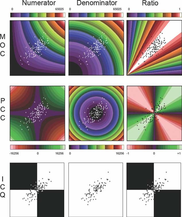
Weighting of the PCC, MOC, and ICQ
The coefficients all use the same data, the intensities of
two fluorophores in homologous pixels. To explore the origins
of the differences between the coefficients, the numerator and
denominator were considered separately and the values for ev-
ery combination of intensities were superimposed on a stand-
Figure 4. Gain. The intensities of one image of a colocalized pair ard scattergram (Fig. 7). This displays the weight attached to
was progressively altered and the response of the PCC and the each combination for the numerator, the denominator and
MOC followed (A). Note that the x-axis has a break The effect of finally shows their combined impact as a ratio (Fig. 7). The
changes in the gain is illustrated by two scattergrams (B). A gain
of 1.0 kept the data at the limits of the 8-bit range. In addition to
numerator of the PCC is based on the difference from the
varying the gain the effect of including noise that is independent population mean and is nonlinear. The maximum weight of
of the gain is shown. The noise was added after any alteration in 116,256 applies to a pair of intensities at either the upper or
the gain and had a uniform distribution with different widths,
lower limits of the intensity range, while pairs with values at
which are marked on the PCC plots. For reasons of clarity, the
noise levels are not marked on the MOC plots, but correspond to the population mean carry no weight (zero). Since the PCC
those of the PCC. The original images had a mean intensity of 128 employs the difference from the mean, every positive weight-
and a Gaussian distribution with a width of 28. ing has a matching negative weighting. The MOC employs the
absolute intensity, making every weighting positive, and is also
nonlinear. A pair of intensities in the midrange have only a
themselves uncorrelated, produces an overall positive correla-
quarter of the weight (16,256) of a pair at the top of the range
tion: a combination of two uncorrelated populations produces
(65,025), while a combination of low intensities has little
a positive PCC (Fig. 5A).
influence. The numerator of the ICQ is binary, either the dif-
When the replacement population of pixels has a mean in-
ferences from the mean have the same sign or they do not.
tensity equal to that of the original population, rather than a
The denominator is similar to the numerator with a non-
lower intensity, the pattern of change is reversed (Fig. 5B), the
linear pattern for the MOC and PCC. The pattern seen in the
PCC remains unchanged while the MOC increases, most
denominator and in the numerator are similar for the MOC,
noticeably when the correlation (negative copy fractions) is
but are quite different for the PCC. The denominator for the
negative.
ICQ is unweighted, every pixel pair has the same weight.
The ratio (numerator/denominator) shows combinations
Multiple Relationships: Combining Two that the coefficients treat as having a similar degree of colocali-
Correlated Subsets zation. The ratios show that both the PCC and the MOC have
Combining two correlated sets of pixels into a single quite a broad band of maximal colocalization, where small
population reduces the measured PCC and MOC, with the changes to the intensities have little effect on the ratio. The
greater reduction in the PCC (Fig. 5C). The second-correlated surrounding gradient is relatively gentle for the MOC but
population was produced by reducing the intensity of a subset changes more sharply for the PCC. Note that the ‘‘ratio’’
Cytometry Part A 77A: 733742, 2010 737ORIGINAL ARTICLE
panels on the right display areas of equal colocalization but shows that almost all the points fall into the highly colocalized
that the numerator provides a better indication of the weight category for MOC whereas with the PCC they spread more
given to different combinations of intensities in the overall cal- widely, illustrating why the MOC returns high values and is
culation: for the MOC, a high- and low-intensity pair may be unresponsive to changes in the data. The ratio for the ICQ is
equally colocalized but the high intensity carries a heavy identical to the numerator.
weight whereas the low-intensity pair has a negligible influ- The weights for the SRC were not calculated because the
ence. The scattergram, that was overlayed on the ratio panels, pattern, although basically similar to the PCC, will vary
between datasets, an effect of ranking.
DISCUSSION
It is self-evidently worthwhile to quantify colocalization
but the plethora of available coefficients (PCC, MOC, ICQ,
SRC, M1, M2, k1, and k2) and their differing meanings, can be
confusing. We have made a detailed examination of two of the
coefficients used for correlation measurements, the PCC and
its derivative the MOC, to establish how they work and
whether they are useful. The two coefficients are almost identi-
cal and differ only in the use of the absolute intensity, by the
MOC, or the deviation from the mean, by the PCC, a small
but significant change.
The MOC was created as an improvement on the PCC, to
be ‘‘. . .especially applicable when the intensities of the fluores-
cence of detected antigens differ’’ (12) and because the PCC
‘‘is not sensitive to differences in signal intensity between the
components of an image caused by different labeling with
fluorochromes, photobleaching or different settings of ampli-
fiers’’ (1), claims that have been repeated uncritically (5,11).
We find that both the PCC and MOC are, within wide limits,
independent of the magnitude of the signal. Therefore, the
major claim made for the MOC falls.
Two further coefficients, k1 and k2, were derived from the
MOC, by using only the intensity of one fluorophore in the
denominator (1). The product of the intensities of both fluor-
ophores is then related to the intensity of a single fluorophore,
hence the need for two coefficients. Absolute intensity is em-
bedded in the k1 and k2 coefficients, but image acquisition is
almost always adjusted to fit the detector’s response range and
the actual intensities have little meaning. k1 and k2 really
require the actual number of molecules present in each pixel.
Even comparisons between cells imaged under standard con-
ditions are problematic because uptake and expression of fluo-
rescent molecules varies widely. The k1 and k2 seem to have no
Figure 5. Colocalization and multiple relationships. The PCC and
the MOC are affected by the presence of a subpopulation with a
different degree of colocalization. In the upper panel (A) the sub-
population is uncorrelated and of low intensity, intended to emu-
late the inclusion of background pixels. The size of the subpopula-
tion is expressed as a percentage of the whole population and the
colocalization of the main population was varied by changing the
copy fraction (see Fig. 1A). The MOC was unaffected even when
background pixels formed 25% of the whole population and inter-
mediate values are not shown. In the middle panel (B) the subpo-
pulation has a mean equal to that of the main population. The
bottom two panels (C) include a second correlated subpopulation,
which is illustrated by the scattergram. The changes in gain
(x-axis) apply only to the subpopulation and the size of subpopu-
lation is shown as percentage of the total.
738 Quantifying ColocalizationORIGINAL ARTICLE
Figure 7. The weightings inherent in the PCC, the MOC and the
ICQ for every combination of intensities found in an 8-bit range
and based on the numerator and denominator of Eqs. (1), (2), and
(3). Two false color scales are used, a red-blue-green scale that
covers negative values and a rainbow scale for positive range.
The ICQ range is binary, with white for 1 and black for 0. The
values for an 8-bit intensity range are shown adjacent to each
false color scale. A scattergram is superimposed.
Figure 6. Effect of a single datapoint. One datapoint was moved
radially about the mean of an uncorrelated population. Radii of
90, 70, 50, 30, and 10 were used, which are marked on the scatter- Offset has a differential effect on the PCC and the MOC.
gram. The start position (angle of zero) is shown by the base of
the arrow, which also shows the rotation direction. The peak The PCC is completely independent of shifts in the signal but
response was seen with the largest radius (90). The scales used the MOC can either increase or, more surprisingly, be
for each coefficient cover an equal fraction of the full response. decreased, by positive offsets. The MOC works because the
product of the intensities (the numerator) is less than or equal
advantages over the M1 and the M2 coefficients that were con- to the denominator. A positive offset increases the numerator
currently launched (1). M1 and M2 calculate for each fluoro- more than it increases the denominator and the MOC rises. A
phore the fraction of the total intensity that co-occurs. The fall in the MOC after a positive offset to one of the images is
absolute values of k1 and k2 would only become meaningful if therefore unexpected. It arises when the correlation is negative
intensities were replaced by an estimate of the number of and high intensities in one image correspond to low intensities
molecules present. However, even photon counting methods in the second image, and vice versa. Then, the increase in the
are not used routinely in biological imaging and estimating numerator is less than the increase in the denominator and
the number of molecules is difficult. the MOC falls. An increase in the MOC followed by a progres-
Table 1. Comparison of correlation coefficients
PCC MOC ICQ SRC
Theoretical range 21 to 11 0 to 11 20.5 to 10.5 21 to 11
Gain Independent Independent Independent Independent
Offset background subtraction Unimportant Important Unimportant Unimportant
Weighting Departure from the mean Magnitude None Departure from mean rank
Inclusion of background pixels Sensitive Insensitive Sensitive Sensitive
Inclusion of midrange pixels Insensitive Sensitive Sensitive Slightly sensitive
Sensitivity to correlation Good Poor Good Good
Cytometry Part A 77A: 733742, 2010 739ORIGINAL ARTICLE
sive fall is also possible when a single image is offset. This combinations, where one or both of the pair is/are of a low in-
occurs with low intensities, low enough that the product with tensity, have little influence on the numerator and a small
homologous pixels is nearly zero, and when a small increase, influence on the denominator. This seems like an attractive
say from 1 to 2, has a bigger effect on the numerator than on feature, for a correlation coefficient, but a strong correlation
the denominator. In this limited sense, the MOC is sensitive to requires that a match exists across the whole intensity range,
the absolute signal. It is therefore important that the offset be including low intensities and the MOC is blind in this region.
set correctly, i.e., zero fluorescence produces zero detection. One high-intensity pair can produce a MOC that is almost
Correctly setting the offset is important since the position of unaffected by any number of blank or low-intensity combina-
the intercept contains useful information: a line that does not tions, which undermines its value as an overlap coefficient and
pass through the origin indicates that part of the fluorescence makes the MOC a poor measure of co-occurrence. The biggest
is independent of the second fluorophore and of the correla- difference between the MOC and the PCC is apparent in the
tion between the two fluorophores. Since the size of any offset pattern of weightings for the numerator and denominator,
is not reported by the PCC, it could be considered a limitation. they are similar for the MOC but differ with the PCC. The ra-
The inclusion of uncorrelated pixels with low intensities, tio of the numerator to the denominator shows one main axis
which emulate background pixels, has a profound effect on for the MOC but two axes for the PCC, one strongly negative.
the PCC but leaves the MOC unchanged. The PCC becomes This makes the PCC an effective measure of correlation. The
more positive and the effect on low or negatively correlated different pattern of weighting explains the quite different
PCCs is substantial even when the percentage of background meanings of a coefficient of zero: the PCC reports zero when
pixels is very small. The practical consequences are that the there is no relationship between the intensities whereas the
accurate measurement of the PCC requires the exclusion of MOC reports zero only when the two fluorophores totally
background pixels, which should be standard practice. The avoid each other.
failure to exclude pixels devoid of fluorescence transforms an The SRC is attractive because, unlike the PCC, it does not
apparently uncorrelated relationship into a highly positive require a normally distributed population, a prerequisite that
PCC (10). The corollary is that pixels with intensities close to many biological specimens may not meet. The SRC also detects
the mean affect the MOC but not PCC. nonlinear correlations and is less sensitive to outlying datapoints
Combining two positively correlated populations appre- than the PCC (8,9). It might be good practice to compare SRC
ciably reduces both the PCC and the MOC, although the abso- and PCC and examine the raw data should they differ.
lute change in the MOC is smaller. This is a limitation of both A new correlation method that counts only whether
coefficients. The coefficients summarize what may actually be intensities are above or below the mean has been developed
a complex relationship that might include differently corre- (6). The ICQ method simply expresses the number of match-
lated subpopulations and nonlinear relationships. The PCC ing pixels, when both are either above or below their mean, as
underestimates nonlinear relationships and the rank Spear- a fraction of the total, and then subtracts 0.5. The subtraction
man coefficient is a viable alternative (8,9). The original ensures that negative correlations have a negative quotient,
images and the scattergram should always be examined, even within a 20.5 to 10.5 scale. This scale differs from the more
though visual assessment is imperfect (13). common 21 to 11 generally used for correlation. A remedy is
When a scattergram suggests a complex relationship, it is simply to double the ICQ (15). The ICQ is a simple and there-
tempting to select and then separately analyze any subpopula- fore intelligible coefficient. The disadvantage is that pixels
tion (14). However, this is a fundamental error in data analy- marginally above the mean carry exactly the same weight as
sis, since the selection of the subpopulation is based on the pixels with more extreme intensities. Therefore, the ICQ is
very relationship for which an objective measurement is sensitive to changes in pairs of pixels that fall near the mean
required. A legitimate alternative is to select biologically intensity of either fluorophore. By comparison, the PCC is
meaningful areas for analysis, e.g., individual cells rather than almost unaffected by changes in this subset of pixels. Surpris-
a tissue or to separate the cytoplasm from the nucleus. This ingly, the ICQ was not rigorously compared with established
might initially involve selecting a distribution from the scatter- coefficients when introduced (6). The ICQ performed well
gram and establishing its spatial origin in the specimen, but if over the range of correlations produced by changing the copy
a physiologically relevant area is highlighted then all the pixels fraction, being similar to the PCC and SRC. A tendency to flip
in that area must be considered in the correlation analysis, i.e., between values was seen when a single pixel was moved and
if the ‘‘interesting’’ pixels come from the cell nucleus it is not examination of the weightings suggests that there are datasets,
legitimate to analyze only the selected pixels. which could undergo substantial changes without affecting the
The explanation for the different properties and sensitiv- ICQ. The ICQ is nevertheless an interesting innovation.
ities of the PCC and the MOC lies in the different weighting A mistake often arises when two fluorophores that do not
given to the intensities of the two fluorophores. Since the PCC co-occur, with perhaps one in the cytoplasm and the other in
is based on differences from the mean, intensity pairs near the the nucleus, are nonetheless tested for correlation. The PCC
mean are of little consequence whereas those at the extremes then reports a negative correlation, whereas the MOC reports
of the intensity range are highly influential (8), hence the con- a plausibly low value, the one occasion it delivers. This PCC is
sequences of including background pixels. In the MOC, com- clearly spurious but these negative correlations are not always
binations of high intensities carry significant weight while recognized as artifacts (10). It is important to differentiate
740 Quantifying ColocalizationORIGINAL ARTICLE
between a true negative correlation, where high intensities are A more pertinent consideration is the accuracy and precision
matched with low intensities, and this ‘‘not in the same place’’ with which measurements can be made. It is acknowledged
error. The lack of co-occurrence could be detected by the M1 that the quality of the images influences the accuracy of colo-
and M2 coefficients. We strongly advocate thresholding to calization measurements (1,16,20) and that noise reduces the
exclude pixels which do not contain both fluorophores and measured colocalization. A correction for noise has been
the separate analysis of biologically distinct regions. Automatic demonstrated for the PCC and SRC (8,21). The MOC is as
thresholding, using the idea that the background pixels are insensitive to noise as to most other features of the data.
uncorrelated (16) or based on the background mean and Overall, the PCC and the MOC produce values that differ
standard deviation, are alternatives to operator controlled widely for both the simulated datasets we have employed and
thresholding. with biological images (15,22) and there is little correlation
The MOC is considered to be easier to interpret than the between these two measures of correlation. The PCC does
PCC since it only reports positive values (4,5). Since negative cor- measure correlation, the degree to which the intensity varia-
relations can arise, for example, an enzyme that converts a fluo- tions of one fluorophore follows variation in the second fluor-
rescent molecule into a nonfluorescent form, quenching, FRET or ophore, but since only pixels containing both signals are ana-
localized avoidance, it seems appropriate to record them. The ori- lyzed, the PCC should be qualified by the M1 and M2 coeffi-
ginal case for the MOC ‘‘the negative values of the correlation cients, which report the fraction of the total intensity that
coefficient (PCC) are difficult to interpret when the degree of co-occur (1,23). The MOC provides a highly weighted mea-
overlap is the quantity to be measured’’ (1) is much more re- sure of co-occurrence, is also affected by correlation and is
stricted and includes the important caveat ‘‘when the degree of sensitive to offset. For measurements of co-occurrence, the
overlap is of interest.’’ Like many caveats, this one has been over- MOC should be replaced by M1 and M2. Given that colocaliza-
looked in the discussion of the PCC and the MOC (4,5). tion is well supplied with coefficients, it would be productive
The question arises as to what specifically ‘‘overlap’’ refers to abandon the MOC and the related k1 and k2 pair of coeffi-
to in the context of the MOC, it remains undefined in the ori- cients. The PCC, SRC, and perhaps the ICQ provide useful
ginal article (1), unless the equation for the MOC is taken to measures of correlation (Table 1).
be the definition and ‘‘an overlap coefficient equal to 0.5
implies that 50% of both components of the image overlap’’ is Additional Equations
accepted, a claim for which there appears to be no justifica- P
tion. The assumption is that overlap is some measure of the ðRi Þ:ðGi Þ
k1 ¼ P 2
degree of similarity in the distribution of two fluorophores, Ri :
but the MOC is a curious hybrid measure combining elements P
of correlation with a highly weighted form of co-occurrence. It ðRi Þ:ðGi Þ
k2 ¼ P 2
is in no way comparable with either the percentage of pixels in Gi :
which co-occurrence is found nor to the M1 and M2, coeffi- P
R
cients which report the fraction of each fluorophore’s intensity M1 ¼ Pi;coloc
that co-occurs. R1
It has been suggested that a threshold exists for values of
the PCC (10,12) and the MOC (12) that mark biologically
meaningful colocalization and, conversely, below which colo- Ri,coloc is the intensity of the red fluorophore in pixels
calization is deemed unimportant. It has been stated that no where the green fluorophore is present.
conclusions can be drawn from a PCC between 20.5 and 0.5 P
G
(10) and the MOC’s threshold is apparently 0.6, for which no M2 ¼ P i;coloc
supporting evidence or rationale has been presented (12). Our G1
results show that a MOC of \0.6 cannot be obtained even
from datasets that show minimal or even negative correlation Gi,coloc is the intensity of the green fluorophore in pixels
and that low values of the PCC have biological meaning (17). where the red fluorophore is present.
Even after randomly shuffling the pixel intensities, the MOC
can still return values above 0.6 while randomization, predic-
LITERATURE CITED
tably, reduces the PCC to zero but more surprisingly leaves the 1. Manders EMM, Verbeek FJ, Aten JA. Measurement of co-localization of objects in
ICQ positive (15). However, since the PCC and MOC are dual-colour confocal images. J Microscopy 1993;169:375–382.
2. Gillham EM. A Life of Sir Francis Galton, Oxford: Oxford University Press; 2001.
graded measures the very idea of a threshold is strange (18), 3. Manders EM, Stap J, Brakenhoff GJ, van Driel R, Aten JA. Dynamics of three-dimen-
especially for values close to the nominal threshold, where a sional replication patterns during the S-phase, analysed by double labelling of DNA
and confocal microscopy. J Cell Sci 1992;103 (Pt 3):857–862.
minor shift in the measurement would reverse the interpreta- 4. Zinchuk V, Zinchuk O, Okada T. Quantitative colocalization analysis of multicolor
tion. The relevant biological consideration is whether the confocal immunofluorescence microscopy images: Pushing pixels to explore biologi-
cal phenomena. Acta Histochem Cytochem 2007;40:101–111.
measured colocalization is changed experimentally. Even small 5. MediaCybernetics. Colocalization of fluorescent probes. Available at: http://www.
changes ‘‘half an eye is just 1% better than 49% of an eye’’ mediacy.com/pdfs/colocfluorprobes.pdf; 2002. pp1–5.
(Richard Dawkins) and ‘‘information is any difference that 6. Li Q, Lau A, Morris TJ, Guo L, Fordyce CB, Stanley EF. A syntaxin 1, Galpha(o), and
N-type calcium channel complex at a presynaptic nerve terminal: Analysis by quanti-
makes a difference’’ (Gregory Bateson) (19) can be important. tative immunocolocalization. J Neurosci 2004;24:4070–4081.
Cytometry Part A 77A: 733742, 2010 741ORIGINAL ARTICLE
7. Khanna R, Sun L, Li Q, Guo L, Stanley EF. Long splice variant N type calcium chan- single axon terminals during postnatal development of mouse neocortex: A quantita-
nels are clustered at presynaptic transmitter release sites without modular adaptor tive analysis with correlation coefficient. Eur J Neurosci 2007;26:3054–3067.
proteins. Neuroscience 2006;138:1115–1125. 16. Costes SV, Daelemans D, Cho EH, Dobbin Z, Pavlakis G, Lockett S. Automatic and
8. Adler J, Pagakis SN, Parmryd I. Replicate-based noise corrected correlation for accu- quantitative measurement of protein-protein colocalization in live cells. Biophys J
rate measurements of colocalization. J Microsc 2008;230 (Pt 1):121–133. 2004;86:3993–4003.
9. French AP, Mills S, Swarup R, Bennett MJ, Pridmore TP. Colocalization of fluorescent 17. Parmryd I, Adler J, Patel R, Magee AI. Imaging metabolism of phosphatidylinositol
markers in confocal microscope images of plant cells. Nat Protoc 2008;3:619–628. 4,5-bisphosphate in T-cell GM1-enriched domains containing Ras proteins. Exp Cell
10. Bolte S, Cordelieres FP. A guided tour into subcellular colocalization analysis in light Res 2003;285:27–38.
microscopy. J Microsc 2006;224:213–232. 18. Adler J, Parmryd I. In support of the Pearson correlation coefficient. J Microsc 2007;
11. Oheim M, Li D. Quantitative colocalisation imaging: Concepts measurements and 227 (Pt 1):83.
pitfalls. In: Shorte SL, Frischknecht F, editors. Imaging Cellular and Molecular Bio-
19. Kay A. Computer software. Sci Am 1984;251:41–47.
logical Functions. Springer; 2007. pp 117–155.
12. Zinchuk V, Grossenbacher-Zinchuk O. Recent advances in quantitative colocalization 20. Demandlox D, Davoust J. Multicolour analysis and local image correlation in confo-
analysis: Focus on neuroscience. Prog Histochem Cytochem 2009;44:125–172. cal microscopy. J Microscopy 1997;185:21–36.
13. Cleveland WS, Diaconis P, Mcgill R. Variables on scatterplots look more highly corre- 21. Adler J, Bergholm F, Pagakis SN, Parmryd I. Noise and colocalization in fluorescence
lated when the scales are increased. Science 1982;216:1138–1141. microscopy: Solving a problem. Microsc Anal 2008;155:7–10.
14. Penarrubia PG, Ruiz XF, Galvez J. Quantitative analysis of the factors that affect the 22. Galloway S, Takechi R, Pallebage-Gamarallage MM, Dhaliwal SS, Mamo JC. Amy-
determination of colocalization coefficients in dual-color confocal images. IEEE loid-beta colocalizes with apolipoprotein B in absorptive cells of the small intestine.
Trans Image Process 2005;14:1151–1158. Lipids Health Dis 2009;8:46.
15. Nakamura K, Watakabe A, Hioki H, Fujiyama F, Tanaka Y, Yamamori T, Kaneko T. 23. Smallcombe A, McMillan D. Co-localisation: How is it determined, and how is it
Transiently increased colocalization of vesicular glutamate transporters 1 and 2 at analysed with the Bio-Rad LaserPic image analysis software. Bio-Rad. pp1–8.
742 Quantifying ColocalizationYou can also read


