Consensus Based Medical Image Segmentation Using Semi-Supervised Learning And Graph Cuts
←
→
Page content transcription
If your browser does not render page correctly, please read the page content below
Consensus Based Medical Image Segmentation Using
                                               Semi-Supervised Learning And Graph Cuts

                                                                          Dwarikanath Mahapatra
arXiv:1612.02166v3 [cs.CV] 21 May 2018

                                                              IBM Research - Australia, Melbourne, Australia.
                                                                         dwarim@au1.ibm.com

                                         Abstract
                                         Medical image segmentation requires consensus ground truth segmentations to
                                         be derived from multiple expert annotations. A novel approach is proposed
                                         that obtains consensus segmentations from experts using graph cuts (GC) and
                                         semi supervised learning (SSL). Popular approaches use iterative Expectation
                                         Maximization (EM) to estimate the final annotation and quantify annotator’s
                                         performance. Such techniques pose the risk of getting trapped in local minima.
                                         We propose a self consistency (SC) score to quantify annotator consistency
                                         using low level image features. SSL is used to predict missing annotations
                                         by considering global features and local image consistency. The SC score also
                                         serves as the penalty cost in a second order Markov random field (MRF) cost
                                         function optimized using graph cuts to derive the final consensus label. Graph
                                         cut obtains a global maximum without an iterative procedure. Experimental
                                         results on synthetic images, real data of Crohn’s disease patients and retinal
                                         images show our final segmentation to be accurate and more consistent than
                                         competing methods.
                                         Keywords: Multiple experts, Segmentation, Crohn’s Disease, Retina,
                                         Self-consistency, Semi supervised learning, Graph cuts.

                                         1. Introduction

                                             Combining manual annotations from multiple experts is important in medi-
                                         cal image segmentation and computer aided diagnosis (CAD) tasks such as per-
                                         formance evaluation of different registration or segmentation algorithms, or to
                                         assess the annotation quality of different raters through inter- and intra-expert
                                         variability [1]. Accuracy of the final (or consensus) segmentation determines
                                         to a large extent the accuracy of (semi-) automated segmentation and disease
                                         detection algorithms.
                                             It is common for medical datasets to have annotations from different ex-
                                         perts. Combining many experts’ annotations is challenging due to their varying
                                         expertise levels, intra- and inter-expert variability, and missing labels of one or
                                         more experts. Poor consensus segmentations seriously affect the performance

                                         Preprint submitted to Elsevier                                         May 22, 2018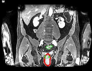
of segmentation algorithms, and robust fusion methods are crucial to their suc-
cess. In this work we propose to combine multiple expert annotations using
semi-supervised learning (SSL) and graph cuts (GC). Its effectiveness is demon-
strated on example annotations of Crohn’s Disease (CD) patients on abdominal
magnetic resonance (MR) images, retinal fundus images, and synthetic images.
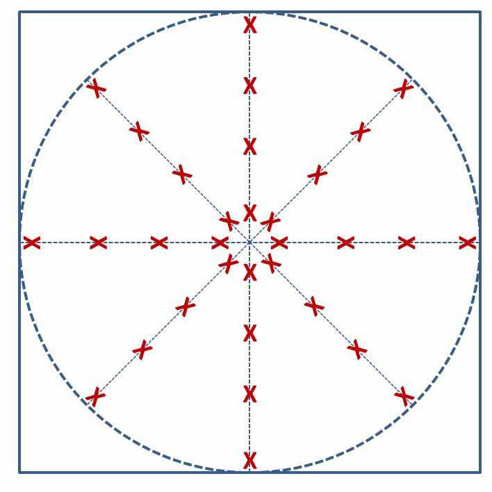
Figure 1 shows an example with two consecutive slices of a patient affected with
CD. In both slices, the red contour indicates a diseased region annotated by
Expert 1 while green contour denotes diseased regions annotated by Expert 2.
Two significant observations can be made: 1) in Figure 1 (a) there is no com-
mon region which is marked as diseased by both experts; 2) in Figure 1 (b) the
area agreed by both experts as diseased is very small. Figure 1 (c) illustrates
the challenges in retinal fundus images where different experts have different
contours for the optical cup. The challenges of intra- and inter-expert variabil-
ity are addressed by a novel self-consistency (SC) score and the missing label
information is predicted using SSL.
1.1. Related Work
Fusing expert annotations involves quantifying annotator performance. Global
scores of segmentation quality for label fusion were proposed in [2, 3]. However,
as suggested by Restif in [4] the computation of local performance is a better
measure since it suits applications requiring varying accuracy in different image
areas. Majority voting has also been used for fusing atlases of the brain in [5].
However, it is limited by the use of a global metric for template selection which
considers each voxel independently from others, and assumes equal contribution
by each template to the final segmentation. It also produces locally inconsistent
segmentations in regions of high anatomical variability and poor registration.
To address these limitations weighted majority voting was proposed in [6] that
calculates weights based on intensity differences. This strategy depends on in-
tensity normalization and image registration and is error prone.
A widely used algorithm for label fusion is STAPLE [3] that uses Expectation-
Maximization (EM) to find sensitivity and specificity values maximizing the
data likelihood. These values quantify the quality of expert segmentations.
Their performance varies depending upon annotation accuracy, or anatomical
variability between templates [7]. Commowick et al. propose Local MAP STA-
PLE (LMSTAPLE) [8] that addresses the limitations of STAPLE by using slid-
ing windows and Maximum A Posteriori (MAP) estimation, and defining a prior
over expert performance. Wang et al. [9] exploit the correlation between dif-
ferent experts through a joint probabilistic model for improved automatic brain
segmentation. Chatelain et al. in [10] use Random forests (RF) to determine
most coherent expert decisions with respect to the image by defining a consis-
tency measure based on information gain. They select the most relevant features
to train the classifier, and do not combine multiple expert labels. Statistical ap-
proaches such as COLLATE [11] model the rating behavior of experts and use
statistical analysis to quantify their reliability. The final annotation is obtained
using EM. The SIMPLE method combines atlas fusion and weight selection in
2
an iterative procedure [12]. Combining multiple atlases demonstrates the im-
portance of anatomical information from multiple sources in segmentation tasks
leading to reduced error compared to a single training atlas [13, 14].

1.2. Our Contribution
    The disadvantage of EM based methods is greater computation time, and
the risk of being trapped in local minimum. Consequently, the quantification
of expert performance might be prone to errors. Statistical methods such as
[15] require many simulated user studies to learn rater behavior, which may be
biased towards the simulated data.
    Another common issue is missing annotation information from one or more
experts. It is common practice to annotate only the interesting regions in medi-
cal images such as diseased regions or boundaries of an organ and disagreement
between experts is a common occurrence. However in some cases we find that
one or more experts do not provide any labels in some image slices, perhaps due
to mistakes or inattention induced due to stress. In such cases it is important to
infer the missing annotations and gather as much information as possible since it
is bound to impact the quality of the consensus annotation. Methods like STA-
PLE predict missing labels that would maximize the assumed data likelihood
function, which seems to be a strong assumption on the data distribution.
    Our work addresses the above limitations through the following contribu-
tions:
  1. SSL is used to predict missing annotation information. While SSL is a
     widely used concept in machine learning it has not been previously used
     to predict missing annotations. Such an approach reduces the computa-
     tion time since it predicts the labels in one step without any iterations as in
     EM based methods. By considering local pixel characteristics and global
     image information from the available labeled samples, SSL predicts miss-
     ing annotations using global information but without making any strong
     assumptions of the form of the data generating function.
  2. A SC score based on image features that best separate different train-
     ing data quantifies the reliability and accuracy of each annotation. This
     includes both local and global information in quantifying segmentation
     quality.
  3. Graph cuts (GC) are used to obtain the final segmentation which gives a
     global optimum of the second order MRF cost function and also incorpo-
     rates spatial constraints into the final solution. The SC is used to calculate
     the penalty costs for each possible class as reference model distributions
     cannot be defined in the absence of true label information. GC also pose
     minimal risk of being trapped in local minima compared to previous EM
     based methods.
We describe different aspects of our method in Sections 2-5, present our results
in Section 7 and conclude with Section 8.

                                        3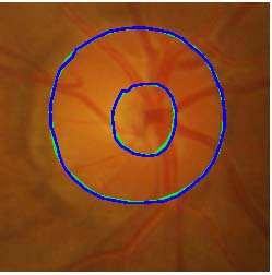
(a)                               (b)                                (c)

Figure 1: (a)-(b) Illustration of subjectivity in annotating medical images. In both figures,
red contour indicates diseased region as annotated by Expert 1 while green contour denotes
diseased region as annotated by Expert 2. (c) outline of optic cup by different experts.

2. Image Features

    Feature vectors derived for each voxel are used to predict any missing an-
notations from one or more experts. Image intensities are normalized to lie
between [0, 1]. Each voxel is described using intensity statistics, texture and
curvature entropy, and spatial context features, and they are extracted from a
31 × 31 patch around each voxel. In previous work [16] we have used this same
set of features to design a fully automated system for detecting and segmenting
CD tissues from abdominal MRI. These patches were used on images of differ-
ent sizes, 400 × 400 and 2896 × 1944 pixels. Through extensive experimental
analysis of the RF based training procedure we identified context features to be
most important followed by curvature, texture and intensity. Our hand crafted
features also outperformed other feature combinations [17]. Since the current
work focuses on a method to combine multiple expert annotations, we refer the
reader to [16] for details.

2.1. Intensity Statistics
    MR images commonly contain regions that do not form distinct spatial pat-
terns but differ in their higher order statistics [18]. Therefore, in addition to the
features processed by the human visual system (HVS), i.e., mean and variance,
we extract skewness and kurtosis values from each voxel’s neighborhood.

2.2. Texture Entropy
    Texture maps are obtained from 2-D Gabor filter banks for each slice (at
orientations 0◦ , 45◦ , 90◦ , 135◦ and scale 0.5, 1). They are partitioned into 9 equal
parts corresponding to 9 sectors of a circle. Figure 2 (a) shows the template
for partitioning a patch into sectors and extracting entropy features. For each
sector we calculate the texture entropy given by,
                                          X
                                χrani = −     prtex log prtex .                     (1)
                                           tex

                                             4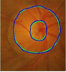
prtex denotes the probability distribution of texture values in sector r. This
procedure is repeated for all the 8 texture maps over 4 orientations and 2 scales
to extract a (8 × 9 =) 72 dimensional feature vector.

2.3. Curvature Entropy
    Different tissue classes have different curvature distributions and we exploit
this characteristic for accurate discrimination between different tissue types.
Curvature maps are obtained from the gradient maps of the tangent along the
3D surface. The second fundamental form (F 2) of these curvature maps is
identical to the Weingarten mapping and the trace of the F 2 matrix gives the
mean curvature. This mean curvature map is used for calculating curvature
entropy. Details on curvature calculation are given in [19, 16]. Similar to texture,
curvature entropy is calculated from 9 sectors of a patch and is given by
                                           X
                                  r
                             Curvani  =−       prθ log prθ .                     (2)
                                             θ

prθdenotes the probability distribution of curvature values in sector r, θ denotes
the curvature values. Intensity, texture and curvature features combined give a
85 dimensional feature vector.
   We use 2D texture and curvature maps as the 3D maps do not provide
consistent features because of lower resolution in the z direction compared to
the x and y axis (voxel resolution was 1.02 × 1.02 × 2.0 mm). Experimental
results demonstrate that using 2D features results in higher classification accu-
racy (82%) in identifying diseased and normal samples when compared to using
3D features (76%). We also resample the images using isotropic sampling and
extract 3D features, but the results are similar and favour the use of 2D features.

2.4. Spatial Context Features:
    Context information is particularly important for medical images because
of the regular arrangement of human organs [20, 21]. Figure 2 (b) shows the
template for context information where the circle center is the current voxel and
the sampled points are identified by a red ‘X’. At each point corresponding to
a ‘X’ we extract a 3 × 3 region and calculate the mean intensity, texture and
curvature values. The texture values were derived from the texture maps at 90◦
orientation and scale 1. The ‘X’s are located at distances of 3, 8, 15, 22 pixels
from the center, and the angle between consecutive rays is 45◦ . The values from
the 32 regions are concatenated into a 96 dimensional feature vector, and the
final feature vector has 96 + 85 = 181 values. The choice of sampling distances
and angles was determined experimentally on a small subset of images, with
3, 8, 15, 22 pixels and 45◦ giving the best result in distinguishing between normal
and diseased samples.

                                         5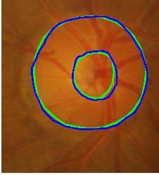
(a)                     (b)

Figure 2: (a) partitioning of patch for calculating anisotropy features; (b) template for calcu-
lating context features.

3. Learning Using Random Forests

   Let us consider a multi-supervised learning scenario with a training set S =
{(xn , yn1 , · · · , ynr )}R                                                 r
                           r=1 of samples xn , and the corresponding labels yn provided
by R experts. A binary decision tree is a collection of nodes and leaves with
each node containing a weak classifier that separates the data into two subsets of
lower entropy. Training a node j on Sj ⊂ S consists of finding the parameters of
the weak classifier that maximize the information gain (IGL ) of splitting labeled
samples Sj into Sk and Sl :

                                                   |Sk |          |Sl |
                IGj,L (Sj , Sk , Sl ) = H(Sj ) −         H(Sk ) −       H(Sl )              (3)
                                                    Sj             Sj

where H(Si ) is the empiric entropy of Si , and |.| denotes cardinality. The
parameters of the optimized weak classifier are stored in the node. Data splitting
stops when we reach a predefined maximal depth, or when the training subset
does not contain enough samples. In this case, a leaf is created that stores the
empiric class posterior distribution estimated from this subset.
   A collection of decorrelated decision trees increases generalization power over
individual trees. Randomness is introduced by training each tree on a random
subset of the whole training set (bagging), and by optimizing each node over a
random subspace of the feature parameter space. At testing time, the output of
the forest is defined as the average of the probabilistic predictions of the T trees.
Note that the feature vector for every pixel consists of the features defined in
Section 2.

3.1. Predicting Missing Labels
     Missing labels are commonly encountered when multiple experts annotate
data. We use semi-supervised learning (SSL) to predict the missing labels.
Unlike previous methods ([22]), a ‘single shot’ RF method for SSL without the
need for iterative retraining was introduced in [23]. We use this SSL classifier as
it is shown to outperform other approaches [23]. For SSL the objective function
encourages separation of the labeled training data and simultaneously separates

                                               6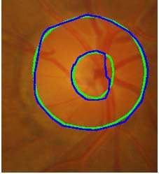
different high density regions. It is achieved via the following mixed information
gain for node j:
                           IGj,SSL = IGj,UL + αIGj,L                           (4)
where IGj,L is defined in Eqn. 3. Ij,UL depends on both labeled and unlabeled
data, and is defined using differential entropies over continuous parameters as
                                             X |Sji |
                   Ij,UL = log |Λ(Sj )| −             log |Λ(Sj )|             (5)
                                               |Sj |
                                            i∈{k,l}

Λ is the covariance matrix of the assumed multivariate distributions at each
node. For further details we refer the reader to [23]. Thus the above cost
function is able to combine the information gain from labeled and unlabeled
data without the need for an iterative procedure.
    Each voxel has r(≤ R) known labels and the unknown R − r labels are
predicted by SSL. The feature vectors of all samples (labeled and unlabeled) are
inputted to the RF-SSL classifier which returns the missing labels. Note that
although the same sample (hence feature vector) has multiple labels, RF-SSL
treats it as another sample with similar feature values. The missing labels are
predicted based on the split configuration (of decision trees in RFs) that leads
to maximal global information gain. Hence the prediction of missing labels is
not directly influenced by the other labels of the same sample but takes into
account global label information [23].

4. Self Consistency of Experts

    Since the annotator is guided by visual features, such as intensity, in distin-
guishing between different regions, it is expected that for reliable annotations
the region with a particular label would have consistent feature distributions.
Expert reliability is quantified by examining the information gain at different
nodes while training a random forest on samples labeled by a particular expert.
This helps us evaluate the consistency of the experts with respect to the visual
features. For each expert r we define an estimator E b r of the expectation of the
                                                      j
information gain on the labeled training set Sj sent to node j as
                               X
                      bjr = 1
                      E          IGrj,L (Sj , Sk (θ), Sl (θ))                  (6)
                            Θj
                                θ∈Θj

where Θ is a randomly selected subset of the feature parameters space. E        br
                                                                                 j
measures how well the data can be separated according to the labels of each
expert. However, it suffers from two weaknesses in lower nodes of the tree:
(i) it is evaluated from fewer samples, and hence becomes less reliable, and
(ii) it quantifies only the experts’ local consistency, without considering global
consistency measures. Therefore, similar to [10] we define the performance level

                                        7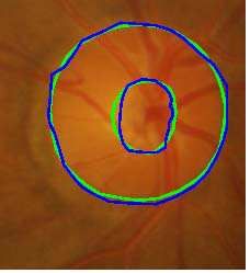
b r from root to node
qjr of each expert as a linear combination of the estimators Ej
j as
                                    PD(j)      br
                                r     d=0 |Sd |Eid (j)
                               qj =   PD(j)            .                       (7)
                                         d=0 |Sd |
    By weighting the estimators in proportion to the size of the training subset,
we give more importance to the global estimates of the experts’ consistencies,
but still take into account their feature-specific performances. Once the param-
eters qjr have been computed, an expert’s reliability or self consistency (SC r ) is
calculated as the average performance level over all nodes j in T trees:
                                           P r
                                      r      j qj
                                   SC =                                         (8)
                                             T
where T is the total number of trees in the forest. Higher SC r indicates greater
rater consistency. To reduce computation time we select a region of interest
(ROI) by taking the union of all expert annotations and determining its bound-
ing box rectangle. The size of the rectangle is expanded by ±20 pixels along
rows and columns and ±2 slices to give the final ROI.

5. Obtaining Final Annotations

   The final annotation is obtained by optimising a second order MRF cost
function that is given by,
                           X             X
                    E(L) =    D(Ls ) + λ       V (Ls , Lt ),          (9)
                              s∈P             (s,t)∈Ns

where P denotes the set of pixels; Ns is the 8 neighbors of pixel s (or sample x);
Ls is the label of s; t is the neighbor of s, and L is the set of labels for all s. λ =
0.06 determines the relative contribution of penalty cost (D) and smoothness
cost (V ). We have only 2 labels (Ls = 1/0 for object/background), although
our method can also be applied to the multi-label scenario. The final labels are
obtained by graph cut optimization using Boykov’s α−expansion method. For
details about the implementation we refer the reader to [24].
    The penalty cost for MRF is usually calculated with respect to a reference
model of each class (e.g., distribution of intensity values). The implicit assump-
tion is that the annotators’ labels are correct. However, we aim to determine
the actual labels of each pixel and hence do not have access to true class dis-
tributions. To overcome this problem we use the consistency scores of experts
to determine the penalty costs for a voxel. Each voxel has R labels (after pre-
dicting the missing labels). Say for voxel x the label y r (of the rth expert) is 1,
and the corresponding SC score is SCxr (Eqn.8). Since SC is higher for better
agreement with labels, the corresponding penalty cost for Lx = 1 is

                              D(Lx = 1)r = 1 − SCxr ,                             (10)

                                          8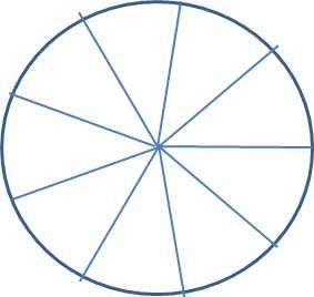
where Lx is the label of voxel x. Consequently, the corresponding penalty cost
for label 0 is
                    D(Lx = 0)r = 1 − D(Lx = 1) = SCxr .                   (11)
However, if the label y r (of the rth expert) is 0, then the corresponding penalty
costs are as follows
                    D(Lx = 0)r = 1 − SCxr ,
                                                                             (12)
                    D(Lx = 1)r = 1 − D(Lx = 0) = SCxr .
The individual penalty costs depend upon the labels given by the experts, while
the final penalty costs for each Lx is the average of costs from all experts,
                                        PR
                       D(Lx = 1) = R1 r=1 D(Lx = 1)r ,
                                        PR                                    (13)
                       D(Lx = 0) = R1 r=1 D(Lx = 0)r .

    Smoothness Cost (V): V ensures a spatially smooth solution by penalizing
discontinuities. We used a standard and popular formulation of the smoothness
cost as originally proposed in [24]. It is given by
                                  ( (Is −It )2
                                   e− 2σ2 · ks−tk1
                                                    , Ls 6= Lt ,
                   V (Ls , Lt ) =                                        (14)
                                   0                  Ls = Lt .

I denotes the intensity. Smoothness cost is determined over a 8 neighborhood
system.

6. Dataset Description
   We use real datasets from two different applications: 1) Crohn’s disease
detection, and 2) colour fundus retinal images originally intended for optic cup
and disc segmentation, and a synthetic image dataset. Details of the different
datasets are given below.

6.1. Crohn’s Disease Dataset
    For Crohn’s Disease we use datasets from two different sources, one from the
Academic Medical Center (AM C), Amsterdam and the other from University
College of London Hospital (U CL).

   • AM C: The data was acquired from 25 patients (mean age 38 years, range,
     25.6 − 59.6 years, 15 females) with luminal Crohn’s disease that had been
     approved by AMC’s Medical Ethics Committee. All patients had given
     informed consent to the prior study. Patients fasted four hours before a
     scan and drank 1600 ml of Mannitol (2.5%) (Baxter, Utrecht, the Nether-
     lands) one hour before a scan. T −1 weighted images were acquired using a
     3-T MR imaging unit (Intera, Philips Healthcare, Best, The Netherlands)
     with a 16-channel torso phased array body coil. The image resolution
     was 1.02 mm × 1.02 mm× 2 mm/pixel, and the volume dimension was
     400 × 400 × 100 pixels.

                                        9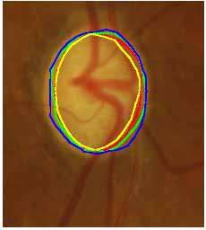
• U CL: Data from 25 patients (mean age, 29.7 years, range, 17.4 − 54.3
     years, 12 females) diagnosed with small bowel Crohn’s disease was used.
     T −1 weighted images were acquired using a 3T MR imaging unit (Avanto;
     Siemens, Erlangen). The spatial resolution of the images was 1.02 mm
     × 1.02 mm× 2 mm per pixel. Two datasets have dimension of 512 × 416 ×
     48, one 512 × 416 × 64, one 512 × 512 × 56 and the rest 512 × 512 × 48.
     Ethical permission was given by the University College London Hospital
     ethics committee, and informed written consent was obtained from all
     participants.

    Each of the hospital MRI datasets was annotated by 4 radiologists, two each
from AMC and UCL. Consensus segmentations were obtained using 4 methods
described in Section 7.5. The final segmentations of all 50 patients are used to
train a fully supervised method for detecting and segmenting CD tissues (details
are given in Section 6.3) using 5−fold cross validation.

6.2. Colour fundus retinal images
    We use the DRISHTI-GS dataset [25] consisting of retinal fundus images
from 50 patients obtained using 30 degree FOV at a resolution of 2896 × 1944
pixels. The optic cup and optic disc are manually segmented by 3 ophthalmol-
ogists, and the consensus ground truth is also available. We choose this dataset
because the final ground truth and annotations of individual experts are publicly
available and facilitates accurate validation.

6.3. Evaluation Metrics
    Availability of ground truth annotations makes it easier to evaluate the per-
formance of any segmentation algorithm. However, the purpose of our exper-
iments is to estimate the actual ground truth annotations, and hence there is
no direct method to estimate the accuracy of the consensus annotations. We
adopt the following validation strategy using a fully supervised learning (FSL)
framework:
  1. Obtain the consensus segmentation from different methods.
  2. Train a separate RF classifier on the consensus segmentations of different
     methods in a 5−fold cross validation setting. The same set of features as
     described in Section 2 are used to describe each voxel. If the training labels
     were obtained using STAPLE then the FSL segmentation of the test image
     is compared with the ground truth segmentation from STAPLE only.
  3. Use the trained RF classifiers to generate probability maps for each voxel
     of the test image.
  4. Use the probability maps to obtain the final segmentation using the fol-
     lowing second order MRF cost function

                  X                                  X             (Is −It )2          1
         E(L) =         − log (P r(Ls ) + ǫ) + λ              e−      2σ2       ·           ,   (15)
                                                                                    ks − tk
                  s∈P                              (s,t)∈Ns

                                          10
where P r is the likelihood (from probability maps) previously obtained
using RF classifiers and ǫ = 0.00001 is a very small value to ensure that
the cost is a real number. The smoothness cost is same as Eqn 14.
5. Obtain the final segmentation using graph cuts. Note that this segmen-
tation is part of the validation scheme and not for obtaining consensus
annotations.
This validation is similar to our previous method in [16], but without using
the supervoxels for region of interest detection. The algorithm segmentations
are compared with the ‘ground-truth’ segmentations (the consensus segmenta-
tion obtained by the particular method) using Dice Metric (DM) and Hausdorff
distance (HD). Consensus segmentations with greater accuracy give better dis-
criminative features and more accurate probability maps, and the classifiers
obtained from these annotations can identify diseased regions more accurately.
Thus we expect the resulting segmentations to be more accurate. The fusion
method which most effectively combines the different annotations is expected
to give higher accuracy for the segmentations on the test data.
Dice Metric measures the overlap between the segmented diseased region
obtained by our algorithm and reference manual annotations. It is given by
2 |A ∩ M |
DM = , (16)
|A| + |M |
where A - segmentation from our algorithm and M - manual annotations. The
DM measure yields values between 0 and 1 where high DM corresponds to a
good segmentation.
Hausdorff Distance (HD): HD measures the distance between the con-
tours corresponding to different segmentations. If two curves are represented
as sets of points A = {a1 , a2 , · · · .} and M = {m1 , m2 , · · · .}, where each ai and
mj is an ordered pair of the x and y coordinates of a point on the curve, the
distance to the closest point (DCP) for ai to the curve M is calculated. The
HD, defined as the maximum of the DCP’s between the two curves, is:
HD(A, M ) = max(maxi {DCP (ai , M )},
(17)
maxj {DCP (mj , A)}).
The results between two different methods were compared using a paired
t−test with a 5% significance level that determines whether the two sets of
results are statistically different or not. MATLAB’s ttest2 function was used as
it because it integrates better into our workflow and the result is returned as the
p−value. Before performing the t−test we ensured that all essential assumptions
are met namely, 1) all measurements are on a continuous scale; 2) the values
are from a related group; 3) no significant outliers are present; 4) assumption
of normality is not violated.
Our whole pipeline was implemented in MATLAB on a 2.66 GHz quad core
CPU running Windows 7 with 4 GB RAM. The random forest code was a MAT-
LAB interface to the code in [26] written in the R programming language.The
RF classifier had 50 trees and its maximal tree depth was 20.
11Table 1: Change in segmentation accuracy with different values of λ (Eqn. 9). DM is in %.
λ 10 5 1 0.5 0.1 0.06 0.02 0.01 0.001
DM 71.4 72.8 75.4 80.2 82.8 88.7 87.2 87.4 86.1
7. Experiments and Results
7.1. Inter-expert Agreement
Each of the hospital MRI datasets was annotated by 4 radiologists, two
each from AMC and UCL. Thus each slice has 4 different annotations and a
mean annotation is calculated from them. The average DM between individual
annotations and mean annotations was 91.5 (minimum DM= 88.4 and maxi-
mum DM= 94.3). The corresponding average p values from the paired t−test
between the mean annotation of the individual annotations of that slice was
p = 0.5241 (minimum p = 0.1978, maximum p = 0.5467). The corresponding
numbers for inter-expert agreement on retinal images was average DM= 94.3
(minimum DM= 90.6 and maximum DM= 96.0), and average p = 0.6124 (min
p = 0.4582, max p = 0.6715). These values indicate good agreement between
different experts. Since each expert annotated a slice only once we do not have
the appropriate data to calculate intra-expert agreement.
7.2. MRF regularization strength λ (Eqn. 9)
To choose the MRF regularization strength λ we choose a separate group of
7 patient volumes (from both hospitals), and perform segmentation using our
proposed method but with λ taking different values from 10 to 0.001. The results
are summarized in Table 1. The maximum average segmentation accuracy using
Dice Metric (DM) was obtained for λ = 0.06 which was fixed for subsequent
experiments. Note that these 7 datasets were a mix of patients from the two
hospitals and not part of the test dataset used for evaluating our algorithm.
7.3. Influence of Number of Trees
The effect of the number of trees (NT ) on the segmentation is evaluated by
varying them and observing the final segmentation accuracy (DM values) on
the 7 datasets mentioned above. The results are summarized in Table 2. For
NT > 50 there is no significant increase in DM (p > 0.41) but the training
time increases significantly. The best trade-off between NT and DM is achieved
for 50 trees and is the reason behind our choice in the RF ensemble. The tree
depth was fixed at 20 after cross validation comparing tree depth, and resulting
classification accuracy.
7.4. Synthetic Image Dataset
To illustrate the relevance of the SC score, we report segmentation results
on synthetic images as they provide a certain degree of control on image char-
acteristics. Figure 3 (a) shows an example synthetic image where the ‘diseased’
12Table 2: Effect of number of trees in RF classifiers (NT ) on segmentation accuracy and training
time (TT r ) of RF − SSL. DM is in %.
NT 5 7 10 20 50 70 100 150
DM 82.5 84.7 86.6 88.3 91.7 91.8 91.7 91.7
TT r 0.20T 0.21T 0.42T 0.8T T 1.4T 2.2T 3.4T
region is within the red square. Pixel intensities are normalized to [0, 1]. In-
tensities within the square have a normal distribution with µ ∈ [0.6, 0.8] and
different σ. Background pixels have a lower intensity distribution (µ ∈ [0.1, 0.3]
and different σ). 120 such images with different shapes for the diseased region
(e.g., squares, circles, rectangles, polygons, of different dimensions) are created
with known ground truths of the desired segmentation. 15 adjacent boundary
points are chosen and randomly displaced between ±10−20 pixels. This random
displacement is repeated for 2 − 3 more point sets depending on the size of the
image. These multiple displacements of boundary points is the simulated anno-
tation of one annotator. Two other sets of annotations are generated to create
simulated annotations for 3 ‘experts’. The annotations of different experts are
shown as colored contours in Fig. 3 (b).
To test our SSL based prediction strategy, we intentionally removed 1 ex-
pert’s annotations for each image/volume slice. The experts whose annotation
was removed is chosen at random. We refer to our method as GCME (Graph
Cut with Multiple Experts) and compare its performance with the final segmen-
tations obtained using COLLATE [11], Majority Voting (MV) [5], and Local
MAP-STAPLE (LMStaple) [8]. We also show results for GCME−All in which
none of the expert annotations were removed while predicting the final segmen-
tation. Note that except for GCME−All , all other methods don’t have access to
all annotations.
Additionally, we show results for GCME−wSSL , i.e., GCME without SSL for
predicting missing labels. In this case the penalty costs are determined from
SCi ’s of available annotations. Missing annotations of experts is not predicted
and hence not used for determining the consensus segmentation. Consensus
segmentation results are also shown for GCME−wSC , i.e., GCME without our
SC score. The penalty cost is the χ2 distance between the reference distribu-
tion in the ground truth annotation of Fig. 3 (a), and the distribution from
the ‘expert’s’ annotation. Note that this condition can be tested only for syn-
thetic images where we know the pixels’ true labels. For COLLATE we utilized
the implementations available from the MASI fusion package [27]. Local MAP
STAPLE implementation is available from the Computational Radiology Labo-
ratory website [28]. For both methods we closely followed the parameter settings
recommended by the authors.
Table 3 summarizes the performance of different methods. GCME−All gives
the highest DM and lowest HD values, followed by GCME , [8], [11], [5], GCME−wSSL
and GCME−wSC . Our proposed self consistency score accurately quantifies the
consistency level of each expert as is evident from the significant difference in
13(a) (b) (c) (d) (e)
(f) (g) (h) (i)
Figure 3: (a) synthetic image with ground truth segmentation in red; (b) synthetic image
with simulated expert annotations; final segmentation obtained by (c) GCM E (DM= 0.94);
(d) Majority voting (DM= 0.86); (e) COLLATE (DM= 0.89); (f) LMStaple (DM= 0.91); (g)
GCM E−All (DM= 0.96); (h) GCM E−wSSL (DM= 0.83); (i) GCM E−wSC (DM= 0.81).
Table 3: Quantitative measures for segmentation accuracy on synthetic images. DM- Dice
Metric in %; HD is Hausdorff distance mm and p is the result of Student t−tests with respect
to GCM E .
GC GCME LmStaple Collate MV GC GC
ME−All [8] [11] [5] ME−wSSL ME−wSC
DM 92.3 91.2 88.8 87.1 85.3 84.0 83.7
HD 6.1 7.4 9.0 10.1 11.9 13.5 13.9
p 0.032 - < 0.01 < 0.01 < 0.01 < 0.01 < 0.001
performance of GCME and GCME−wSC (p < 0.001). Figures 3 (c)-(i) show the
final segmentations obtained using the different methods.
7.5. Real Patient Crohn’s Disease Dataset
For the CD patient datasets we show consensus segmentation results for
GCME−All , GCME , GCME−wSSL COLLATE, Majority Voting (MV), and LM-
Staple. Although, all the 4 experts annotated every image, in order to test our
SSL based prediction strategy, we intentionally removed 1 or 2 annotations for
each image/volume slice.
Figure 4 shows the predicted ground truth for 6 fusion strategies using only
two expert labels. We show results for two experts due to the ease in showing the
different annotations in one image. Displaying three or more expert annotations
with the consensus segmentation makes the images very crowded and hence
difficult to interpret. Since our purpose is to show the relative merit of different
methods, two expert annotations also serve the same purpose.
14Table 4: Quantitative measures for segmentation accuracy on CD images. DM- Dice Metric
in %; HD is Hausdorff distance in mm and p is the result of Student t−tests with respect to
GCM E .
GC GCME LMSTAPLE COLLATE MV GC
ME−All [8] [11] [5] ME−wSSL
DM 92.6±2.4 91.7±3.0 87.3±4.5 85.1±5.3 83.8±7.3 82.3±9.0
HD 7.4±2.6 8.2±3.3 9.8±4.8 12.0±6.2 13.9±7.4 14.7±8.2
p 0.042 - < 0.01 < 0.01 < 0.01 < 0.01
Figures 5,6 show segmentation results for two patients (U CL Patient 23 and
AM C Patient 15) using all the 6 fusion strategies mentioned above and Table 4
summarizes their average performance over all 50 patients. From the visual re-
sults and quantitative measures it is clear that GCME−All gives the highest DM
and lowest HD values, followed by GCME , [8], [11], [5], and GCME−wSSL . Since
GCME−All had access to all annotations, it obviously performed best. However
GCME ’s performance is very close and a Student t−test with GCME−All gives
p < 0.042 indicating very small difference in the two results. Thus we can
effectively conclude that GCME does a very good job in predicting missing an-
notations. Importantly, GCME performs much better than all other methods
(p < 0.01). The results show SSL effectively predicts missing annotation infor-
mation since GCME−wSSL shows a significant drop in performance from GCME
(p < 0.01).
If the consensus segmentation is inaccurate then the subsequent training is
also flawed because the classifier learns features from many voxels whose label
is inaccurate. As a result, in many cases the final segmentation includes regions
which do not exhibit any disease characteristics as confirmed by our medical
experts. Another limitation of sub-optimal label fusion is the wide variation in
segmentation performance of that particular method. The standard deviation
of [5] is much higher than GCME indicating inconsistent segmentation quality.
A good fusion algorithm should assign lower reliability scores to inconsistent
segmentations, which is achieved by GCME as is evident from the low variation
in its DM scores.
An important factor limiting the performance of LMStaple is its prediction of
sensitivity and specificity parameters from the annotations without considering
their overall consistency. Our SC score takes into account both global and local
information and is able to accurately quantify a rater’s consistency. The effect
of SC is also highlighted through experiments on synthetic images (Section 7.4)
Secondly, LMStaple may be prone to being trapped in local minimum due to the
iterative EM approach. On the contrary, we employ graph cuts which is almost
always guaranteed to give a global minimum. This makes the final output
(the consensus segmentation) much more accurate and robust. COLLATE also
suffers due to its reliance on an EM based approach.
15(a) (b) (c)
(d) (e) (f)
Figure 4: The predicted ground truth for UCL Patient 23 by different methods: (a)
GCM E−All ; (b) GCM E ; (c) [8]; (d) [11]; (e) [5]; and (f) GCM E−wSSL . Red and blue contours
are expert annotations and yellow is the final annotation obtained by the respective methods.
7.6. Real Patient Retina Dataset
Quantitative evaluation is based on F-score and absolute pointwise local-
ization error B in pixels (measured in the radial direction). Additionally we
report the overlap measure S = Area(M ∩ A)/Area(M ∪ A). M is the manual
segmentation while A is the algorithm segmentation. Comparative results are
shown for GCME , GCME−All , GCME−wSSL , COLLATE, MV and LMStaple.
Table 5 summarizes the segmentation performance of different methods. Fig-
ure 7 (b),(c) shows the individual expert annotations and the consensus ground
truth annotation while Figs 7 (d)-(f) show the predicted ground truth for 3 fu-
sion strategies. As is evident from the images GCME shows the best agreement
with the ground truth segmentations.
These results confirm our earlier observations from synthetic and CD patient
datasets about: 1) the superior performance of GCME ; 2) effectiveness of SSL in
predicting missing annotation information; 3) inferior performance of LMStaple
due to predicting sensitivity and specificity parameters from annotations with-
out considering their overall consistency, and using EM; and 4) contribution of
our SC score and graph cuts in obtaining better consensus annotations.
16(a) (b) (c)
(d) (e) (f)
Figure 5: Segmentation results on UCL patient 23 for: (a) GCM E−All ; (b) GCM E ; (c) [8];
(d) [11]; (e) [5]; and (f) (a) GCM E−wSSL ;. Red contour is the corresponding ground truth
generated by the fusion method, and yellow contour is the algorithm segmentation obtained
as described in Section 6.3.
7.7. Computation Time
Since the size of the annotations varies depending on the diseased area (ROI
varies between 70 × 80 to 170 × 200), an average fusion time for an annotation
may be misleading. Therefore we calculate an average fusion time per pixel,
which is the highest for LMStaple at 0.3 seconds followed by COLLATE (0.22
seconds), GCME (0.1 seconds) and majority (voting) MV (0.05 seconds). Other
variations of GCME take almost the same time as GCME . Note that we report
only the time for fusing the annotations and not the total segmentation time as
the segmentation time is the same for all cases since a RF based framework is
used. The segmentation time is an additional 0.2 seconds per pixel.
These results clearly show the faster performance by our method due to
employing SSL and GC for predicting missing annotations and obtaining the
final annotation. The EM based LMStaple algorithm is nearly 3 times slower
than GCME , while COLLATE is 2 times slower because of many computations.
Majority voting is faster than all other methods because of its simple approach
to predicting final annotations. However, its performance is the worst.
17(a) (b) (c)
(d) (e) (f)
Figure 6: Segmentation results on AMC patient 15 for: (a) GCM E−All ; (b) GCM E ; (c) [8];
(d) [11]; (e) [5]; and (f) (a) GCM E−wSSL ;. Red contour is the corresponding ground truth
generated by the fusion method, and yellow contour is the algorithm segmentation obtained
as described in Section 6.3.
8. Discussion And Conclusion
We have proposed a novel strategy for combining multiple annotations and
applied it for segmenting Crohns disease tissues from abdominal MRI, and the
optic cup and disc from retinal fundus images. Qualitative evaluation is per-
formed using a machine learning approach for segmentation. Highest segmen-
tation accuracy is observed for the annotations obtained by our fusion strategy,
which is indicative of better quality annotations. The comparative results of
our method and other fusion strategies highlight the following major points.
1. With least variance of DM values GCME is the most consistent fusion
method, and with highest DM values is also the most accurate.
2. SSL effectively predicts missing annotation information since GCME has
very close performance to GCME−All , and is significantly better than
GCME−wSSL . Local MAP STAPLE infers missing annotations by min-
imising the log-likelhood of the overall cost function. Employing EM con-
tributes to its erroneous results. SSL’s advantage is the predicted anno-
tations are consistent with previously annotated samples by considering
both global information and local feature consistencies.
3. Our proposed self consistency score accurately quantifies the consistency
level of each expert as is evident from the performance of GCME and
18Table 5: Segmentation accuracy of retinal fundus images in terms of F score, overlap and
boundary distance for different methods. B is in pixels; T ime- fusion time in minutes;F -F
score; S-overlap measure; B-boundary error.
GC GC COLLATE LMStaple GC Majority
ME ME−All [11] [8] ME−wSSL Voting
F 95.4 97.2 90.2 89.0 92.1 86.4
S 89.2 91.2 84.8 83.2 85.9 80.8
B 9.9 8.2 13.2 10.9 10.3 18.1
Time 7 7 6 9 7 3
(a) (b) (c) (d) (e)
Figure 7: Example annotations of (a) optic disc and (b) optic cup. The ground truth
consensus segmentation is shown in yellow while the different expert annotations are shown
in red, green and blue. Consensus segmentations for optic cup obtained using (c) GCM E ; (d)
[8]; and (e) [11].
GCME−wSC (p < 0.001) for synthetic images. SC analyses feature distri-
butions of neighboring pixels that share the same labels and gives higher
values for consistent annotations which have similar feature distributions.
4. Graph cut optimization produces a quick global optimum without the
risk of getting trapped in local minimum which can be a serious limitation
for EM based methods. Use of GC and SSL together contribute to low
computation time since there is no iterative approach involved.
Our proposed method for obtaining consensus annotations can be used in
scenarios where there is the need to find a ground truth. In most medical image
analysis applications it is good practice to have 2 or more experts annotate
the images. This also minimizes scope of biased or inaccurate annotations.
In such cases our method can be used to generate the ground truth from the
multiple expert annotations. However, in reality it can be difficult to obtain
multiple expert annotations due to cost and resource issues. In such scenarios
multiple segmentations can be generated from different automatic segmentation
algorithms and the consensus ground truth segmentation can be generated using
our method.
Algorithm Limitations: It is important that in order to generate a good
ground truth we have multiple experts’ annotations. As mentioned before that
it is not easy for many experts to provide annotations. Although in principle
we can use different segmentation algorithms to generate candidate segmenta-
tions and then calculate the ground truth, these algorithms may not always be
accurate and the final result would be erroneous. Thus we see that our algo-
19(a) (b) (c) (d) (e)
Figure 8: Segmentation results for different methods: (a) our proposed GCM E method (b)
[8]; (c) [11]; (d) Majority Voting; and (e) GCM E−All . Green contour is manual segmentation
and blue contours are algorithm segmentations from different fusion methods.
rithm’s performance is limited by the availability of qualified experts to provide
accurate annotations.
SSL for predicting missing annotations is an important part of our fusion
approach and erroneous prediction affects the final results. In SSL the unlabeled
samples are assigned a class based on their presence in the feature space and
its subsequent split to maximize information gain. Erroneous labels of one or
more annotations affects the predicted label. However, our proposed method
limits the damage due to inaccurate label predictions with the help of the SC
score which is based on the image features of each annotation. Inaccurately
labeled annotations are assigned low scores since the image features for a la-
bel are not consistent throughout the annotation. Subsequently, inaccurate or
ambiguous annotations have a lower contribution to the final consensus segmen-
tation. Although we cannot completely eliminate mistakes, use of SC allows us
to minimize them by assigning lower importance to erroneous annotations.
9. References
References
[1] L. Hoyte, W. Ye, L. Brubaker, J. R. Fielding, M. E. Lockhart, M. E.
Heilbrun, M. B. Brown, S. K. Warfield, Segmentations of mri images of the
female pelvic floor: A study of inter and intra-reader reliability., J. Mag.
Res. Imag. 33 (3) (2011) 684–691.
[2] G. Gerig, M. Jomier, M. Chakos, VALMET: A new validation tool for
assessing and improving 3d object segmentation, in: In Proc: MICCAI,
2001, pp. 516–523.
[3] S. Warfield, K. Zhou, W. Wells, Simultaneous truth and performance level
estimation (STAPLE): An algorithm for the validation of image segmenta-
tion., IEEE Trans. Med. Imaging 23 (7) (2004) 903–921.
[4] C. Restif, Revisiting the evaluation of segmentation results: Introducing
confidence maps, in: In Proc: MICCAI, 2007, pp. 588–595.
20[5] P. Aljabar, R. Heckemann, A. Hammers, J. Hajnal, D. R. ., Multi-atlas
based segmentation of brain images:Atlas selection and its effect on accu-
racy., Neuroimage 46 (3) (2009) 726–738.
[6] X. Artaechevarria, A. Munoz-Barrutia., Combination strategies in multi-
atlas image segmentation: Application to brain MR data., IEEE Trans.
Med. Imag. 28 (8) (2009) 1266–1277.
[7] S. Klein, U. van der Heide, I. Lips, M. van Vulpen, M. Staring, J. Pluim.,
Automatic segmentation of the prostate in 3D MR images by atlas matching
using localised mutual information, Medical Physics 35 (4) (2008) 1407–
1417.
[8] O. Commowick, A. Akhondi-Asl, S. Warfield, Estimating a reference stan-
dard segmentation with spatially varying performance parameters: Local
MAP STAPLE., IEEE Trans. Med. Imag. 31 (8) (2012) 1593–1606.
[9] H. Wang, J. Suh, S. Das, J. Pluta, C. Craige, P. Yushkevich, Multi-atlas
segmentation with joint label fusion, IEEE Trans. Patt. Anal. Mach. Intell.
35 (3) (2013) 611–623.
[10] P. Chatelain, O. Pauly, L. Peter, A. Ahmadi, A. Plate, K. Botzel, N. Navab,
Learning from multiple experts with random forests: Application to the
segmentation of the midbrain in 3D ultrasound., in: In Proc: MICCAI
Part II, 2013, pp. 230–237.
[11] A. Asman, B. Landman, Robust statistical label fusion through consensus
level, labeler accuracy, and truth estimation (COLLATE), IEEE Trans.
Med. Imag. 30 (10) (2011) 1779–1794.
[12] T. Langerak, U. van der Heide, A. Kotte, M. Viergever, M. van Vulpen,
J. Pluim, Label fusion in atlas-based segmentation using a selective and
iterative method for performance level estimation (SIMPLE), IEEE Trans.
Med. Imag. 29 (12) (2010) 2000–2008.
[13] M. Sabuncu, B. Yeo, K. V. Leemput, B. Fischl, P. Golland, A generative
model for image segmentation based on label fusion, IEEE Trans. Med.
Imag. 29 (10) (2010) 1714–1729.
[14] J. Lotjonen, R. Wolz, J. Koikkalainen, L. Thurfjell, G. Waldemar, H. Soini-
nen, D. Rueckert, Fast and robust multi-atlas segmentation of brain mag-
netic resonance images, Neuroimage 49 (3) (2010) 2352–2365.
[15] B. Landman, A. Asman, A. Scoggins, J. Bogovic, F. Xing, J. Prince, Robust
statistical fusion of image labels, IEEE Trans. Med. Imag. 31 (2) (2011)
512–522.
[16] D. Mahapatra, P. Schüffler, J.Tielbeek, J. Makanyanga, J. Stoker, S. Tay-
lor, F. Vos, J. Buhmann, Automatic detection and segmentation of crohn’s
disease tissues from abdominal mri., IEEE Trans. Med. Imag. 32 (12) (2013)
1232–1248.
21[17] D. Mahapatra, P. J. Schüffler, J. Tielbeek, J. M. Buhmann, F. M. Vos., A
supervised learning based approach to detect crohn’s disease in abdominal
mr volumes, in: Proc. MICCAI-ABD, 2012, pp. 97–106.
[18] M. Petrou, V. Kovalev, J. Reichenbach, Three-dimensional nonlinear invisi-
ble boundary detection., IEEE Trans. Imag. Proc 15 (10) (2006) 3020–3032.
[19] http://www.cs.ucl.ac.uk/staff/S.Arridge/teaching/ndsp/.
[20] Z. Tu, X. Bai, Auto-context and its application to high-level vision tasks
and 3d brain image segmentation, IEEE Trans. Patt. Anal. Mach. Intell.
32 (10) (2010) 1744 – 1757.
[21] Y. Zheng, A. Barbu, B. Beorgescu, M. Scheuering, D. Comaniciu., Four
chamber heart modeling and automatic segmentation for 3D cardiac CT
volumes using marginal space learning and steerable features., IEEE Trans.
Med. Imag. 27 (11) (2008) 1668–1681.
[22] I. Budvytis, V. Badrinarayanan, R. Cipolla, Semi-supervised video segmen-
tation using tree structured graphical models., in: IEEE CVPR, 2011, pp.
2257–2264.
[23] A. Criminisi, J. Shotton., Decision Forests for Computer Vision and Med-
ical Image Analysis., Springer, 2013.
[24] Y. Boykov, O. Veksler, Fast approximate energy minimization via graph
cuts, IEEE Trans. Pattern Anal. Mach. Intell. 23 (2001) 1222–1239.
[25] J. Sivaswamy, et. al.., Drishti-gs: Retinal image dataset for optic nerve
head(onh) segmentation, in: IEEE EMBC, 2014, pp. 53–56.
[26] A. Liaw, M. Wiener, Classification and regression by randomforest, R News
2 (3) (2002) 18–22.
[27] http://www.nitrc.org/projects/masi fusion/.
[28] http://www.crl.med.harvard.edu/software/.
22You can also read