Who is allowed to see the trees? - A research into the distribution of urban green spaces in Groningen - Student Theses Faculty ...
←
→
Page content transcription
If your browser does not render page correctly, please read the page content below
Who is allowed to see the trees?

A research into the distribution of urban green spaces in
                       Groningen.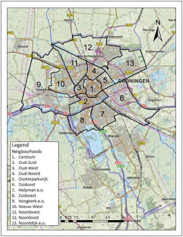
Bachelor Project Victor de Beer | Who is allowed to see the trees? | Version: Final (14-01-2021)

Abstract
This research focuses on the distribution of public urban green spaces (UGS) in the city of
Groningen. The research highlights the importance of UGS in various perspectives. It then
looks into a potential spatial injustice in the distribution of UGS between neighbourhoods with
a lower socio-economic status (SES) and neighbourhoods with higher SES. The main research
question therefore is: ‘How are UGS distributed in comparison to the spatial layout of socio-
economic status in Groningen?’. In order determine the UGS distribution this study looks at
two different indicators: the amount of UGS per person in a neighbourhood, and the percentage
UGS of the total surface of a neighbourhood. The main finding is a pattern of inequality in UGS
distribution between northwest and southeast neighbourhoods. The pattern shows the southern
neighbourhoods generally have higher amounts of UGS than the northern. The overlapping
pattern of this inequality with the spatial distribution of SES, leads this study to presume a
potential form of spatial injustice within the distribution of UGS in Groningen. The study comes
to these results by gathering data from different databases on multiple UGS and SES variables.
Mapping out and analysing these variables determines the values of UGS and SES in the
neighbourhoods.

Key words: urban green spaces (UGS), spatial justice, climate justice, distribution, socio-economic Status
(SES), Groningen.

                                                                                                        2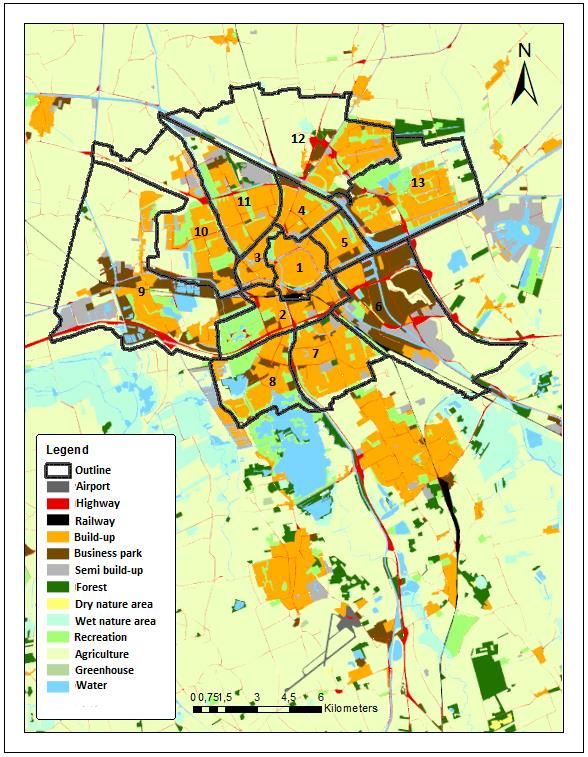
Bachelor Project Victor de Beer | Who is allowed to see the trees? | Version: Final (14-01-2021)

Colophon

Title:                                 Who’s allowed to see the trees?

Author:                                Victor de Beer

Version:                                Final

Words:                                 6592

Date:                                  14-01-2020

Student:                               2574780

Study:                                 BSc Spatial planning and design

Contact:                               v.c.de.beer@student.rug.nl

Organization:                          University of Groningen

Faculty:                               Spatial Sciences

Supervisor:                            dr. Ethemcan Turhan

                                                                                                   3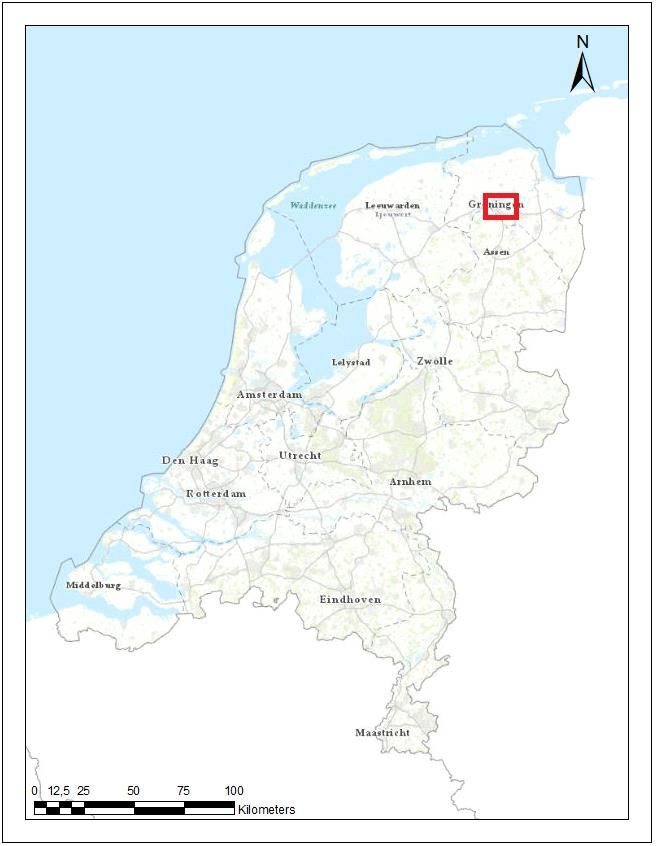
Bachelor Project Victor de Beer | Who is allowed to see the trees? | Version: Final (14-01-2021)

Acronyms

CBS:                                   Centraal Bureau Statistiek (English: Central bureau [of]
Statistics)

GIS:                                   Geographic Information Systems

SES:                                   Socio-economic status

UGS:                                   Urban green spaces

UWV:                                   Uitvoeringsinstituut Werknemersverzekeringen (English:
Employee Insurance Agency)

                                                                                                   4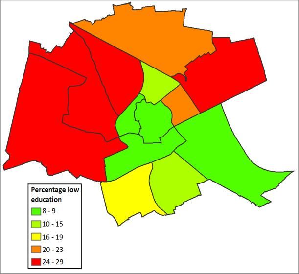
Bachelor Project Victor de Beer | Who is allowed to see the trees? | Version: Final (14-01-2021)

Content
                                                                                     page
1. Introduction……………………………………………...……………. 6

2. Theoretical framework…………………………………………...…… 7

    2.1. Spatial justice………………………………………………..…… 7

    2.2. Socio-economic status………………………………………........ 8

    2.3. Urban green spaces……………………………………………..... 8

    2.4. Spatial injustice in UGS distribution…………………………..… 9

3. Conceptual model……………………………..…………………...…. 9

4. Case Groningen……………………………….………………….…… 10

5. Method………………………………………..…………………….… 11

6. Hypotheses……………………………………………………….…… 12

7. Results……………………………………………………………........ 13

    7.1. Urban green spaces………………………………………….…… 13

    7.2. Socio-economic status……………………………………..…….. 19

    7.3. Spatial justice……………………………………………..……… 22

8. Conclusion…………………………………………………..……...… 25

    10.1. Biases and recommendations…………………………………… 26

9. References………………………………………………………..…… 26

                                                                                                   5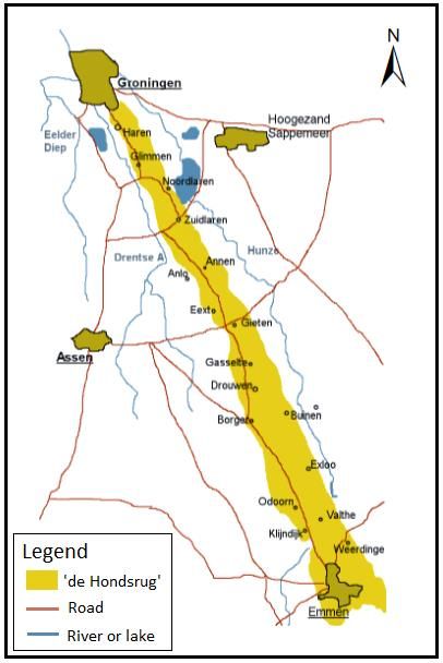
Bachelor Project Victor de Beer | Who is allowed to see the trees? | Version: Final (14-01-2021)
1. Introduction
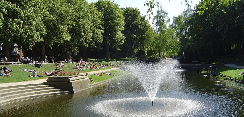
My birth city Groningen has recently been put in a very flattering spotlight. Engineering bureau Arcadis
has determined that Groningen is the healthiest city in the Netherlands (Metro, 2020). The article points
out that Groningen is already working on the physical environment since 1777 in order to prevent disease
outbreaks like the black plague. The result they say is a healthy environment with enough greenery. But
is this greenery accessible for everyone? Considering Nesbitt, Meitner, Girling, Sheppard and Lu (2019,
p 1), who studied the accessibility of urban vegetation in ten cities in the United States, argue that: "For
most cities, the more income and education you had, the more access you had to mixed or woody
vegetation, while parks were more equitably accessible". The quote drew my attention and sparked my
interest in justice in the spatial distribution of urban green spaces (from now on: UGS). Multiple
questions arose: ‘‘Why does this phenomenon happen?’’; ‘‘Does it happen everywhere?’’ and ‘‘Can it
be done in a fair and just way?’’. But above all: ‘‘Is it done in a just way, in my praised hometown,
Groningen?’’
Justice is something mankind has always been preoccupied with, many philosophers are still looking
for the true meaning of justice. Justice has come to us in many forms, in its formal sense as law, and
informally as unwritten moral rules, that form social, economic and, political justice. Social scientists
have been exploring social justice as a way of evaluating the distribution of wealth, income, free time,
health care, and more (G.H. Pirie, 1983). In the same trend some geographers have been exploring the
same notions, but on the basis of spatiality, thereby adopting the notion of spatial injustice. This type of
injustice occurs in the lives of individuals and groups of people on the basis of their spatiality: where
they live, work, travel, etc. And spatial injustice exists in many forms, from an unequal distribution of
UGS to droughts in Chile as a result of lithium extraction (Liu, Agusdinata & Myint, 2019).
A major contributor to spatial injustice is climate change. Its effects are being unequally distributed as
some populations are more vulnerable than others. Since urban green spaces are known to mitigate some
of the consequences of climate change through for example regulating ambient temperatures, filtering
dust, attenuating stormwater, and mitigating flooding (Byrne & Jinjun, 2009), the equal distribution of
UGS is becoming ever more important. Therefore, I want to strike this issue while the iron is hot and
take a look at the distribution of public UGS in my hometown Groningen to provide insight into its
spatial equality. All the more, since the municipality and city administration have ambitious plans when
it comes to creating a greener city (Groenplan Groningen, 2020), I will study if this ‘green city’ is for
everyone and see who is allowed to see the trees.
In short, mankind attaches value to justice, and UGS are of increasing importance. This research,
therefore, focuses on the distribution of public UGS in the city of Groningen. It looks into a potential
spatial injustice between neighbourhoods with different socio-economic statuses (from now on: SES).
The main research question is ‘How are UGS distributed in comparison to the spatial layout of socio-
economic status in Groningen?’ In a broader scope its aim is to provide insight into 1) the spatial
distribution of UGS in the city of Groningen, 2) spatial justice concerning UGS in Groningen and, 3)
contribute to the bigger societal debate on spatial justice specifically concerning UGS. In the following
sections, I will first be providing insight into the relevant concepts and theories in the theoretical
framework. After that, I will provide the significant information of my case: Groningen. Then I will
inform the reader of the methods I will be using, followed by my hypotheses. Hereafter I will be showing
what the distribution of UGS in Groningen looks like, and then see what the different SES levels of the
neighbourhoods are and how they are spatially positioned. This information will be connected in the
final step of my results, and finally, I will close this research with my conclusions.
6
Bachelor Project Victor de Beer | Who is allowed to see the trees? | Version: Final (14-01-2021)

2. Theoretical framework
This theoretical framework will elaborate on three main concepts: spatial justice, SES, and UGS. After
that, the three concepts will be linked together.

2.1 Spatial justice
In his book on the geographical aspect of justice, Seeking Spatial Justice, Edward Soja (2013) makes a
distinction between Justice with a capital J, meaning the justice that comes from law, and there is justice
in the broader sense, meaning the quality of being just or fair. The latter meaning of justice is adopted
in this research. An early researcher to link justice and spatiality in his book Social Needs and Resources
in Local Services, is Michael Davies (1970). He tries to measure how far differences in standards are
related to differences in the relative needs of the population in different local authorities. This led to the
first exploration of spatial justice. Later, Dikeç (2013) builds further upon the notion of justice and its
relation to space and spatiality in his paper Justice and the Spatial Imagination. He says that the
movements of the 1960s and 1970s brought new issues such as ‘rights to the city’ and ‘social justice’ to
our attention. These issues he says, have been influential in almost every discipline including geography
ever since. I will be building upon Soja’s broad and inclusive notion of justice; Micheal Davies’ linkage
between justice and spatiality and Dikeç’ finding that social justice is influential in geography.

A form of spatial justice is environmental justice. Environmental justice looks at the way everyday life
is threatened by environmental risks. These risks, often called hazards, are unjustly distributed. A major
example of this is the inequitable distribution of pollution in the United States, with poor people and
people of colour bearing a greater share than rich and white people (Cole & Foster, 2001).

In their article on the theory and practice of environmental justice, Agyeman, Schlosberg, Craven and
Matthews (2016), point out that environmental justice started out as a movement. Prior, Cole and Foster
(2001) argued that it is impossible to point to a specific date or event that started the movement, as it
grew from hundreds of local conflicts. They describe that there are three big contributors to the
movement, 1) The Civil Rights Movement, 2) The Anti-Toxics Movement and, 3) Academic.
Considering its groundworks, Agyman et al. (2016) do identify a national report called Toxic Wastes
and Race in the United States, on the racial and socio-economic characteristics of communities with
hazardous waste sites, as the first tangible source of data on which the movement based its foundation.

An influential environmental risk is the effects of climate change. The branch of environmental justice
concerning climate change is likewise called climate justice. Crease, Parsons and Fisher (2018) argue
that the impacts of climate change are not distributed evenly within communities in their study on
climate and gender injustices in the Philippines. They also claim that the vulnerability to harm is
differentially distributed. The term vulnerability refers to the degree to which a population manages to
cope with the impacts of climate change (Adger, 1999; O’Brien, Nygaard and Schjolden, 2007).
Therefore, differences in vulnerability will eventually lead to climate injustice. In their review on the
discourse of environmental justice, Schlosberg and Collins (2014) argue that climate justice includes
both distributive and procedural elements. Not only the distribution of environmental goods and harms
between nations, but also the distribution of the impacts of climate change at national and local levels,
and the need for recognition and participation in decision making for all parties. This research will take
a short look at the way UGS plays a role in climate justice and look at the distributive elements that are
pointed out by Schlosberg and Collins (2014) by seeing if the UGS distribution in Groningen is done in
a just way.

                                                                                                            7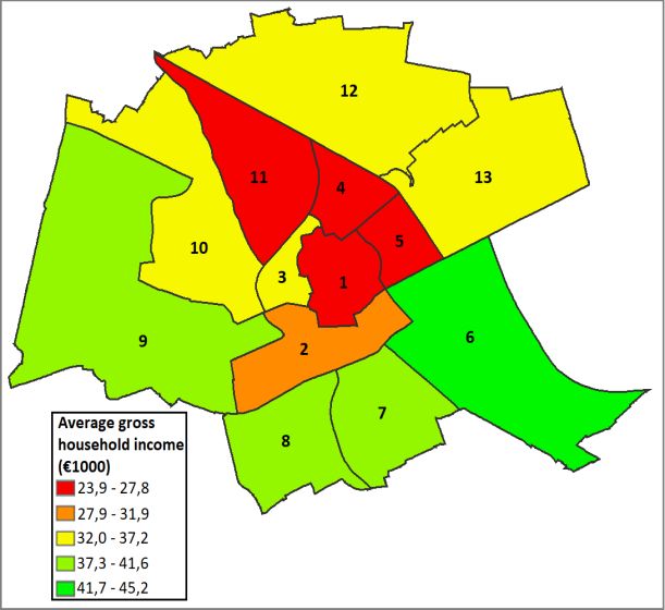
Bachelor Project Victor de Beer | Who is allowed to see the trees? | Version: Final (14-01-2021)

2.2 Social-economic status
This research adopts Chu Lim and Omar Thanoon’s definition of SES. They say that: ‘‘SES is defined
as the position of an individual on a social-economic scale that measures factors such as education,
income, type of occupation, place of residence, and in some populations, heritage and religion’’(2013,
p.15). This status has often been associated with people’s health (Contoyannis & Jones, 2004; Lantz et
al. 1998). Already in an early meta-analysis on three studies, Marmot, Ryff, Bumpass, Shipley and
Marks (1997), concluded that there is a social gradient in mortality studies; mortality, they say, rises
with decreasing socio-economic status. But the scope of associations with SES is broader than just
health, among others, it is also associated with the distribution of UGS. I will elaborate on this in the
last part of this section.

In short, SES is a sizable predictor and indicator of other life factors. It often corresponds with health-
and other indicators. That is why this research will be looking at the connection between the spatial
appropriation of SES and UGS in the neighbourhoods of Groningen.

2.3 Urban green spaces
UGS is made up of public- and private UGS. This study uses the definition of Roy, Byrne and Pickering
(2012, p. 352) on public UGS. In their review of costs and benefits of urban trees, they say it includes
parks and reserves, sporting fields, greenways and trails, community gardens, street trees, riparian areas
like stream- and river banks, green- walls, alleyways, and cemeteries. Private UGS refers to people’s
private property like their backyards. As these are not owned nor planned by the municipality, the study
will not look into them. Public UGS (from now on when UGS is mentioned, I refer to public UGS) have
a wide variety of environmental and social benefits. For instance, UGS function as a local climate
stabilization (Jim & Chen, 2008), they have a cooling effect through the provision of shade (Bowler et
al., 2010) that can have a positive effect on the urban heat island effects, which has also proven to be an
issue in Groningen (RTV Noord, June 8, 2020). Other positive environmental effects are energy
consumption reduction, noise reduction and carbon and water storage (Simpson, 2002; Bolund &
Hunhammar, 1999). Also, social benefits include health improvements like relaxation and stress
reduction associated with UGS exposure (Maas, Verheij, Groenewegen, de Vries & Spreeuwenberg,
2006). Furthermore, use of UGS can lead to an increase in the quality of life by providing a recreational
area for passive and active activities (Byrne & Wolch, 2009).

Thus, UGS have a lot of positive effects on people’s daily lives and cities in general. Therefore, I am
going to take a look at different quantities of UGS in the Groningen neighbourhoods. But in their
literature review on UGS, public health and environmental justice, Wolch, Byrne and Newell (2014),
note that congestions can affect the usage of UGS. Simply put, not only the volume matters, but also the
amount per person also matters. That is why many European cities provide threshold values for per
capita UGS or minimum accessibility for a defined area of UGS. An example of a city using this kind
of threshold is Berlin. According to Kabisch, Strohbach, Haase and Kronenberg (2016, P. 588), Berlin
aims to provide at least 6 m2of UGS per person, while another German city, Leipzig, aims to provide
10 m2of UGS per person. And In the UK, it is recommended that city residents should have access to a
natural green space of minimally 2 ha within a distance of 300 m from home (Handley et al., 2003).
However, Larondelle and Haase (2013), in their cross-analysis on urban ecosystem services, find a
limitation to the pure application of per capita UGS and UGS accessibility threshold value. They say it
can provide a broad assessment of UGS provision, but does not indicate how UGS are distributed across

                                                                                                         8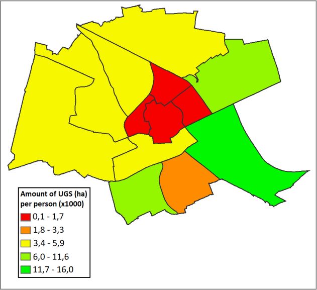
Bachelor Project Victor de Beer | Who is allowed to see the trees? | Version: Final (14-01-2021)

different groups of the society. This shows that it is hard to create the right distribution just by setting a
threshold. Accordingly, this study will try to look at UGS distribution with a broader scope that includes
more indicators on UGS.

Now that I have defined the three main concepts of UGS, SES and spatial justice, I will explain their
connection and possible hiccups in the next section.

2.4 Spatial injustice in UGS distribution
The aforementioned positive effects of UGS highlight the importance of an equal distribution of UGS
across cities to cater everyone with the same benefits. Unfortunately, we see that spatial injustice and
access to UGS are often associated through differences in SES. For example, Wolch et al. (2014) state
that studies reveal that the distribution of UGS often favours communities that are predominantly white
and more affluent.

In their study on deforestation and forest degradation, Bowler et al. (2010) point out that with the current
trend of urban densification, there may be less space for UGS. McPherson (1992), who studied the cost
and benefits of UGS, add to that by arguing that it is harder to increase green infrastructure like UGS in
dense cities. And to make matters worse, when cities do find a way of increasing the supply of UGS, it
might even have a paradoxical effect on poorer neighbourhoods. This paradoxical effect, Wolch et al.
(2014) argue, is that an increase in UGS may lead to an increase in property value and housing costs.
This can lead to so-called ‘green gentrification´. Just like regular gentrification, the increase in housing
costs might push current residents out of their neighbourhoods, and into cheaper neighbourhoods which
are in turn likely to have less. They point out that cities need to focus on strategies that are ‘just green
enough’ in order to prevent green gentrification. The focus needs to be on small scale intervention,
bottom-up green-space strategies supported by anti-gentrification policies like the provision of
affordable housing and housing trust funds. We can conclude that the existence of spatial injustice in
UGS distribution is verified, but with densification of cities, and potential green gentrification, it is
harder than it looks to find possible solutions.

3. Conceptual model

Figure 1. Conceptual model.

                                                                                                            9
Bachelor Project Victor de Beer | Who is allowed to see the trees? | Version: Final (14-01-2021)

In figure 1, you see the way the concepts interact with each other. In the middle is UGS, UGS creates
certain benefits for society on multiple scales. But UGS can be distributed in a certain way, equally and
unequally. This distribution affects the relation between UGS and the benefits; less UGS means fewer
benefits. On the right end we see that when the unequal distribution is grounded on SES we might be
able to talk about spatial injustice. And when it is not based on SES, we can assume that is a regular
deviation from an equal distribution. But there is always external factors, like geography or topology,
we have to take into account as they might play a role in the real-life distribution. When the distribution
is done equally we consider it fair or just in the broader sense of the word mentioned in section 2.1.

4. Case: the city of Groningen
In figure 2 we see Groningen, positioned in the north of the Netherlands. It is the capital of its province,
which is also called Groningen. The city has around 203.000 inhabitants (Alle Cijfers, 2020), with a
significant amount of over 30.000 students (RTV Noord, 2018), due to its university and the
Hanzehogeschool. The city has a total surface of 8372 hectare including 502 hectare of water surface.

Figure 2. Map Netherlands. Edited by author, based on ‘‘Topo RD’’
(Esri Nederland, 2012a).

The CBS (Central Bureau [of] Statistics) has divided Groningen into 14 neighbourhoods (2020). Within
the scope of this research, I will exclude the neighbourhood Meerdorpen, as it has just recently grown
into the agglomeration (Rambharos, 2016). Therefore, it is assumed that the planning of this
neighbourhood is done differently and not by the city of Groningen. Since this is a research into the
planning and structure of neighbourhoods in Groningen, including this neighbourhood would only blur
the results. The remaining 13 neighbourhoods are shown in figure 3.

                                                                                                         10
Bachelor Project Victor de Beer | Who is allowed to see the trees? | Version: Final (14-01-2021)
Figure 3. Map neighbourhoods in Groningen. Created by author, based on ‘‘Open Topo’’ (Esri
Nederland, 2016).
5. Method
In this section I will provide a stepwise overview of the way in which the study will reach its objectives.
Initially, I searched for secondary data on UGS and SES using multiple online databases from CBS.
Since most of the data come from CBS, which is a governmental institution, I can assume that the data
is reliable. The fact that I transformed the data to fit my spatial categorisation might cause some
deterioration due to personal mistakes. This transformation and the rest of the data processing is shown,
schematically, in figure 4. The CBS data is open and reliable data so there is no ethical consideration
11Bachelor Project Victor de Beer | Who is allowed to see the trees? | Version: Final (14-01-2021)
concerning the data. Furthermore, in order to answer the main research question, no additional primary
data is required.
Data Data
Data collection Raw data Data analization
transformation visualization
Figure 4. Schematic visualization of data treatment.
Then, I mapped out an overview of the UGS in Groningen and its general distribution. This map was
used to make preliminary general assumptions about distribution and locations of UGS and other land
uses.
Thirdly, I determined the specific distribution of UGS in the different neighbourhoods. First of all, I
looked at the total amount of UGS. Since just the total amount of UGS does not tell the full story, I then
looked at the percentage UGS take up of the whole neighbourhood surface. The amount of UGS per
person, and the percentage UGS of the total surface for each neighbourhood. The produced data is shown
in multiple figures, tables and maps using ArcGIS and Excel.
After that, the research examined the SES of the thirteen neighbourhoods. I used the variables
percentage of low education inhabitants, average household income and, percentage of work seeking
inhabitants as indicators for the SES of the neighbourhoods. The data is shown in multiple tables, figures
and maps using ArcGIS and Excel.
Concluding this research, I have linked the results of the previous two steps to see if there is a form of
spatial injustice to be found in Groningen.
6. Hypotheses
Since this study is more of a descriptive kind, I do not have any hypotheses. Nevertheless, I do have
some upfront assumptions. Something that has played a major role in the development of the city is the
fact that it is built on the last small tail-end of a ridge called ‘de Hondsrug’ (Huisman, 2003). This ridge,
depicted in figure 6, is higher than its surrounding area, which caused this area to be built up first and,
a better living area to keep dry feet than the surrounding peaty area. This historical fact still influences
the city’s layout to this day, with, as shown in figure 5, southern areas having higher housing prices. I
presume that these southern areas are therefore more likely to have a higher SES. Furthermore, I expect
that I will be able to find a pattern that is similar to the pattern described in the literature review. This
research’s thesis therefore, is that the southern neighbourhoods have higher SES due to its historically
better positioning on ‘de Hondsrug’, creating a division between the south and north. And that, in line
with the literature, inhabitants of these higher SES neighbourhoods in the south have more UGS to their
disposal.
12Bachelor Project Victor de Beer | Who is allowed to see the trees? | Version: Final (14-01-2021)
Figure 5. Map showing average property values in Groningen.
Edited by author, based on ‘‘Gemiddelde WOZ waarde’’
(GronoMeter, 2020).
Figure 6. Map of ‘de Hondsrug’. Edited by author, based
on ‘‘de Hondsrug’’ (Aeroleelde, 2020).
7. Results
7.1 UGS distribution
In this section, I will be showing the distribution of UGS in Groningen. First of all, I will give an
overview of the land-uses in the city. After that, I will provide a table that contains the amounts of
different forms of UGS per neighbourhood. As explained in the literature review, these raw numbers do
not tell the full story of UGS distribution. Therefore I will then provide information on the relative
amounts that the UGS make up of the total surface for each neighbourhood and finally I will put the
amount of UGS in contrast to the number of inhabitants of each neighbourhood. To conclude this chapter
I will give an overview of the previous aspects of UGS to get a clear understanding of its distribution in
Groningen.
The land uses are shown in figure 7. Looking at the map gives a good first impression of the locations
of UGS in Groningen and the division of other land uses.
13Bachelor Project Victor de Beer | Who is allowed to see the trees? | Version: Final (14-01-2021)
Figure 7. Land use in Groningen. Created by author, based on ‘‘Bestand Bodemgebruik 2012’’ (Esri
Nederland, 2012b).
The most striking implications of figure 7 are listed below:
- The centre parts of the city seem to have little UGS.
- The outskirts of the city seem to have more UGS.
- Neighbourhood 6 Zuidoost seems to consist mostly out of business parks and not much
housing.
- A couple of neighbourhoods, 9 Hoogkerk a.s., 10 Nieuw-West, 12 Noordoost and, to a
lesser degree, 13 Noorddijk a.s., seem to include large plots of agricultural land.
14Bachelor Project Victor de Beer | Who is allowed to see the trees? | Version: Final (14-01-2021)
Table 1 shows the distribution of different kinds of UGS across the neighbourhoods.
Table 1. Amounts of different UGS per neighbourhood (Source: OpenData CBS (1,), edited by author)
The main preliminary information that can be drawn from this table is the fact that total amounts of UGS
do not seem equally distributed over the neighbourhoods. With a couple of very high and very low
results, it seems that there is an unequal distribution of UGS in Groningen. We can see that 13 Noorddijk
a.s. and 02 Oud-Zuid have the highest objective scores when it comes to the total amount of UGS.
Furthermore, the neighbourhoods in the city centre: 01 Centrum, 03 Oud-West, 04 Oud-Noord and also
05 Oosterparkwijk seem to be the least endowed.
These divergent results are likely stimulated by diverse total amounts of surface that the neighbourhoods
have. Presumably, the bigger neighbourhoods automatically have bigger amounts of UGS and the other
way around. To check this presumption and to get a clearer picture of the amounts of UGS in a
neighbourhood I take a look at two other variables. First, the amount of UGS divided by the total surface
of the neighbourhood. Secondly, the amount of UGS divided by the number of inhabitants. For the first
variable, it is expected that accounting for the total amount of surface will bring the results closer
together. Also, we saw in figure 3, multiple neighbourhoods: 6 Zuidoost, 9 Hoogkerk a.s., 10 Nieuw-
West and, 12 Noordoost, contain large plots of agricultural land. As I want to know the percentages of
UGS inside the neighbourhoods, the amounts of surface of the agricultural plots will be subtracted from
the total amount of surface of each neighbourhood. This is shown in table 2.
15Bachelor Project Victor de Beer | Who is allowed to see the trees? | Version: Final (14-01-2021)
Table 2. Overview of surface per neighbourhood (Source: OpenData CBS (1), edited by author).
Graph 1 gives us a clearer picture of the neighbourhoods’ spatial makeup. Just like the total amounts of
UGS, the percentages of UGS do not seem equally distributed. But the differences have scaled down
after accounting for the total surface. 02 Oud-Zuid, 08 Zuidwest and, 13 Noorddijk a.s. have
disproportionately large relative amounts of UGS while 03 Oud West, and 09 Hoogkerk a.s. seem to
have relatively fewer UGS.
RELATIVE AMOUNT OF UGS PER
NEIGHBOURHOOD
31,3%
% UGS of surface Average
30,7%
26,3%
20,4%
20,0%
19,0%
15,5%
14,8%
11,3%
16,57%
9,7%
7,9%
6,9%
1,7%
Graph 1. Percentages of different UGS in the neighbourhoods (Source: OpenData CBS (1+2), edited by author).
Finally, we take a look at the amount of UGS per inhabitant. As I explained in the literature review, this
second indicator will give us a better insight into the accessibility of UGS in the neighbourhoods. We
assume that when a lot of people share the same UGS, the accessibility becomes smaller. Graph 2 shows
the per capita values of UGS.
16Bachelor Project Victor de Beer | Who is allowed to see the trees? | Version: Final (14-01-2021)
UGS PER PERSON
UGS per person (x1000) Average
16,0
11,6
9,9
5,9
5,2
5,0
4,9
4,7
5,42
3,3
1,7
1,0
0,8
0,1
Graph 2. Amounts of UGS per inhabitant in the neighbourhoods (Source: OpenData CBS (1+2), edited by author).
We can clearly see some inequality existing in the amount of UGS per person. 06 Zuidoost, 08 Zuidwest
and 13 Noorddijk e.o. have a clear advantage over the rest. In the case of 06 Zuidoost, this results can
mostly be based on the earlier mentioned fact that the neighbourhood is largely made up of industrial
area, thus housing very little inhabitants as can be seen in table 3. This means that the amount of UGS
gets divided by a very little number of inhabitants resulting in the high number. The neighbourhoods 01
Centrum, 03 Oud West, 04 Oud Noord and 05 Oosterparkwijk are clearly showing below average
amounts of UGS per person. As said, I am using the percentage UGS of the total surface and the amount
of UGS per person as main indicators for UGS distribution in Groningen. In order to establish a single
number, I will convert the previous variables into one new indicator. I call this indicator the UGS
distribution level. This will be done by taking the deviations from the mean for every value and adding
those up for each neighbourhood. The new variable is nothing other than an indicator that shows the
differences between the neighbourhoods.
17Bachelor Project Victor de Beer | Who is allowed to see the trees? | Version: Final (14-01-2021)
Table 3. Amounts of inhabitants per neighbourhood
(Source: OpenData CBS (1+2), edited by author).
Table 4. UGS variables per neighbourhood (Source: Open Data CBS (1+2), edited by author).
The maps in figure 8, are a visual representation of the UGS data shown in this chapter. For each
variable, the data is clustered using Jenks Natural Breaks. This is a data clustering method designed to
determine the best arrangement of values into different classes (Jenks, 1967). With these maps, I can
make a global examination of the distribution of UGS over the full city.
18Bachelor Project Victor de Beer | Who is allowed to see the trees? | Version: Final (14-01-2021)
Figure 8. Maps displaying UGS variables. . Created by author, based on ‘‘CBS Wijk- en Buurtkaart 2019’’ (Esri Nederland,
2019).
The trends in UGS distribution can be seen are the following:
- The inner-city neighbourhoods have the lowest values.
- The west, north-western neighbourhoods come second.
- The east, south-eastern parts have the highest values.
- The only exception to these rules seem to be neighbourhood 07 Helpman e.o., this
neighbourhood has an orange/yellow colour in every map, which doesn’t follow the trend of the
surrounding neighbourhoods.
7.2 Social-economic status
In the previous section, I have taken a look into the distribution of UGS to see if this spatial inequality
could be found. In the following section, I will look into the SES of the different neighbourhoods. This
research will be using percentage of low education inhabitants, average household income and
percentage of work seeking inhabitants as indicators for the SES of the neighbourhoods. With three
indicators education, income and, occupation, that cover the aspects in the earlier mentioned definition
19Bachelor Project Victor de Beer | Who is allowed to see the trees? | Version: Final (14-01-2021)
of Chu Lim and Omar Thanoon (p. 8), the span of variables is broad enough to approximate the actual
SES of the neighbourhoods.
I expect to see the different factors of SES to be dependent on each other. That is, if the neighbourhood
has a low SES, the percentage of low educated inhabitants will be high, the household average income
will be low and the percentage work seeking will be high. For high SES neighbourhoods, this pattern is
expected to be the other way around. The different SES factors are shown in table 5. Again, I will
combine these three variables into one, namely SES, by taking the deviation from the mean for every
variable and adding those up. Likewise, the new variable is nothing other than an indicator that shows
the differences between the neighbourhoods.
Table 5. SES values per neighbourhood (Source: OpenData CBS (1+2), edited by author).
As can be seen in table 5, the earlier described SES pattern is often visible. In the table, you can clearly
see that the colour grading for every variable is often more or less the same in one area, which tells us
that the variables are likely to be dependent and therefore a good indication of the actual SES. However,
the first three neighbourhoods seem to be a big exception to this rule. I theorize that this anomaly is due
to the high number of students that live in these neighbourhoods. Students are often not work seeking,
at least not registered at the UWV; they do not have a high income, but they are often highly educated.
This does not follow our regular assumptions of socioeconomic status. Table 6 shows the percentage
15-25-year-old in each neighbourhood, underpinning my theory that a high number of students is the
reason for this result. These atypical data could be seen as outliers. Outliers can significantly affect the
process of estimating statistics (Kwak & Kim, 2017) resulting in a blurring of the results. Removing the
outliers will prevent this from happening. They point out that in order to specify data as an outlier, the
data either needs to be over 3 standard deviations (SD) from the mean or over 1.5 times the quartile
distance from either the first or the third quartile. As you can see in table 6 and figure 9 neither of these
standards for outliers has been met. Therefore, I will not be discarding any of the neighbourhoods.
20Bachelor Project Victor de Beer | Who is allowed to see the trees? | Version: Final (14-01-2021)
Table 6. Percentages 15-25-year-old inhabitants and their SD Figure 9. Boxplot percentages 15-25-year-old
from the mean (Source: OpenData CBS (1+2), edited by author). inhabitants per neighbourhood.
21Bachelor Project Victor de Beer | Who is allowed to see the trees? | Version: Final (14-01-2021)
The maps shown in figure 10 visualise the data on SES.
Figure 10.Maps showing the different SES indicators for the neighbourhoods in Groningen. Created by author, based on
‘‘CBS Wijk- en Buurtkaart 2019’’ (Esri Nederland, 2019).
We can see some general patterns when it comes to the SES of neighbourhoods in Groningen:
- The inner-city neighbourhoods, 01 Centrum, 02 Oud-Zuid and, 03 Oud-West, are a clear
exception to the rule.
- The northern parts of Groningen have a disadvantage when it comes to SES. We also see that
neighbourhood 13 Noorddijk e.o. is now part of this cluster.
- The southern neighbourhoods have a higher SES than the northern neighbourhoods.
In the next section I will determine whether these differences in SES are spatially related to the
distribution of UGS.
7.3 Spatial justice
In the previous sections, I have explained and visualised how UGS are spatially distributed in
Groningen. Then I analysed what the SES of the different neighbourhoods is and showed how this is
spatially distributed. In this section, I explain if we can speak of spatial injustice by seeing if the UGS
22Bachelor Project Victor de Beer | Who is allowed to see the trees? | Version: Final (14-01-2021)
distribution is spatially related to the SES of the neighbourhoods. The data that is gathered in this
research is not applicable for quantitative data analysis. First of all, because this study contains 13 – the
number of neighbourhoods – cases, while qualitative research often needs 30 or more cases. And second
of all because the data is not independent. Simply put, what happens in one neighbourhood affects what
happens in the next neighbourhood. Whereas with qualitative data analysis, the data is presumed to be
independent. Therefore, the following analysis will be an analysis without any real statistical
significance. The results, of course, can still show general patterns and indicators of spatial injustice.
In order to see if there is spatial injustice in the city of Groningen I will see if the following pattern can
be established:
1. In neighbourhoods with relatively low SES is relatively low UGS distribution.
2. In neighbourhoods with relatively high SES there is relatively high UGS distribution.
3. This pattern can be seen across multiple neighbourhoods in the same area.
To check the first to presumptions I will display the different SES statistics compared to the UGS level
in
Infographic 1. Visualization of the UGS level against the percentage low educated inhabitants per neighbourhood.
Infographic 2. Visualization of the UGS level against the percentage work seeking inhabitants per neighbourhood.
23Bachelor Project Victor de Beer | Who is allowed to see the trees? | Version: Final (14-01-2021)
Infographic 3. Visualization of the UGS level against the average household income per neighbourhood.
Infographic 1. Visualization of the UGS level against the SES per neighbourhood.
In two of the three cases, we can see a trend that we expect to see, following my presumptions. Only in
infographic 1, we can see a pattern in which there is more UGS for neighbourhoods that have a higher
percentage of low educated inhabitants. In infographic 2, we do see the trend, neighbourhoods with
more people that are work seeking, are likely to have less UGS. And likewise, in infographic 3, we see
a pattern that follows our presumption, the higher the amount of household income, the higher the
amount of UGS in the neighbourhood. Also in infographic 4, that shows the SES variable I computed
against the UGS level, there is a small trend to be seen that goes along with the presumptions. I cannot,
because of earlier discussed limitations to the data, put any significance to these trends. But the spread
of the points in the graphs does suggest that if there are any real relations, they are most likely very
weak.
The infographics do not suggest a clear pattern but do suggest some weak form of injustice. To see if
this trend can be found across multiple neighbourhoods in the same area, I have done a hot-spot analysis.
The output of this analysis is shown in figure 11. The map is created out of different layers of the hot-
spot analysis for every variable. The analysis tells us where high and low values cluster spatially. In
other words, it tells us where ‘bad’ and ‘good’, SES and UGS results, spatially cluster. The tool does so
by looking at the neighbourhoods within the context of the surrounding neighbourhoods. So, if a
neighbourhood with low UGS is situated in an area where other neighbourhoods also have low UGS, it
is more likely to turn up blue. This also goes the other way around. But if a neighbourhood has low UGS
in an area where other neighbourhoods do not have low UGS, it will likely not turn up blue. This creates
24Bachelor Project Victor de Beer | Who is allowed to see the trees? | Version: Final (14-01-2021)
a analysis that goes beyond the neighbourhood border. Normally the hot-spot analysis required 30 cases.
Therefore, again, I cannot presume the outcome to have a true statistical meaning. The colour-trend that
is shown, however, is still of value.
Figure 11. Map showing the hotspot analysis. . Created by author, based on ‘‘CBS Wijk- en
Buurtkaart 2019’’ (Esri Nederland, 2019).
The hot-spot analysis shows that the northern neighbourhoods seem to be worse off when it comes to
the combination of SES and UGS: they have a lower SES and lower amounts of UGS. This also points
toward a trend of spatial injustice.
8. Conclusion
The main research question for this research asked how UGS are distributed in Groningen, in relation
to the spatial layout of SES. The answer to this question also confirms my thesis. It seems that the higher
lying areas, build on the ‘Hondsrug’ in the south, have a higher SES than the northern areas. And
generally, these higher lying areas also have more UGS to their disposal. The research was also able to
fulfill some of its broader aims, stated in the introduction. Firstly, it has provided insight into the spatial
distribution of UGS in the city of Groningen. However, it cannot come to an unambiguous answer to
the question on spatial justice concerning UGS distribution, but does reveal some general trend. In my
opinion it has also contributed to the bigger societal debate on spatial justice concerning UGS.
As said this research was not able to indicate exact statistical values due to the form of data that was
gathered. Another limitation of the study is the fact that it did not account for the perceived accessibility
of the UGS. Moreover, I feel that the study is very reliant on the way the neighborhoods are drawn up.
This research has found indicators of spatial injustice. It seems that the northern neighbourhoods have
lower average SES and lower average amounts of UGS than the southern neighbourhoods. There are
multiple other possible explanations for these indicators. Preventing green gentrification, explained on
page nine, for example, could be a reasoning behind the decision making on UGS distribution. This is
25Bachelor Project Victor de Beer | Who is allowed to see the trees? | Version: Final (14-01-2021)
also one of the weaker aspects of this study, it does not account for different explanations of unequal
UGS distribution. But as it is a study into the global trends, it does not limit its findings.
Also, the spatial injustice indicator do not seem to have a strong enough relation to be able to speak
about real spatial injustice in Groningen. This study tried to overcome this limitation by doing a hot-
spot analysis, but I would still recommend future studies to look at different spatial appropriations than
just neighbourhoods. Another recommendation for future studies to do a broader study that includes
multiple cities in the Netherlands to be able to get at least 30 cases. This could also be done by doing
research on another spatial scale.
8.1 Conflict of interest or biases
There are no indications of any conflicts of interests in this research. I am aware of some biases that
might be included in this research because of the fact that I was an inhabitant of the city of Groningen
for many years. These biases might have steered me into a direction that wanted to confirm my
presumptions of some neighbourhoods. For example, it is common fact in Groningen that the
neighbourhoods in the south are ‘richer’ than those in the north. These kinds of pre-existing knowledge
might have steered the research in a certain direction.
9. References
Adger, W.N., 1999. Social vulnerability to climate change and extremes in coastal Vietnam.
World development, 27(2), pp.249-269.
Agyeman, J., Schlosberg, D., Craven, L. and Matthews, C., 2016. Trends and directions in
environmental justice: from inequity to everyday life, community, and just sustainabilities.
Annual Review of Environment and Resources, 41.
Aeroeelde., 2020. Rondvlucht Hondsrug. Retrieved on October 26, 2020 via:
https://www.aeroeelde.nl/rondvluchten/hondsrugvlucht
Bolund, P. and Hunhammar, S., 1999. Ecosystem services in urban areas. Ecological
economics, 29(2), pp.293-301.
Bowler, D., Buyung-Ali, L., Healey, J.R., Jones, J.P., Knight, T. and Pullin, A.S., 2010. The
evidence base for community forest management as a mechanism for supplying global
environmental benefits and improving local welfare. CEE review, pp.08-011.
Byrne, J. and Jinjun, Y., 2009. Can urban greenspace combat climate change? Towards a
subtropical cities research agenda. Australian Planner, 46(4), pp.36-43.
26Bachelor Project Victor de Beer | Who is allowed to see the trees? | Version: Final (14-01-2021)
Byrne, J., Wolch, J. and Zhang, J., 2009. Planning for environmental justice in an urban
national park. Journal of Environmental Planning and Management, 52(3), pp.365-392
Cole, L.W. and Foster, S.R., 2001. From the ground up: Environmental racism and the rise of
the environmental justice movement (Vol. 34). NYU Press.
Contoyannis, P., and A.M. Jones. "Socio-economic status, health and lifestyle." Journal of
health economics 23, no. 5 (2004): 965-995.
Crease, R., Parsons, M. and Fisher, K., 2018. " No climate justice without gender justice":
Explorations of the intersections between gender and climate injustices in climate adaptation
actions in the Philippines. Routledge Handbook of Climate Justice.
Davies, B. P. (1968). Social needs and resources in local services: A study of variations in
provision of social services between local authority areas.
Dikeç, M., 2001. Justice and the spatial imagination. Environment and planning A 33, no. 10:
1785-1805.
Esri Nederland., 2012a. Topo RD. Retrieved on October 31, 2020 via:
https://www.arcgis.com/home/item.html?id=1d1d425122e74d4d87695e163f3f10ce
Esri Nederland., 2012b. Bestand Bodemgebruik 2012. Retrieved on October 27, 2020 via:
https://www.arcgis.com/home/item.html?id=dbd0851ae4624cc9b4aadfb0681d4a2f
Esri Nederland., 2016. Open Topo. Retrieved on October 15, 2020 via:
https://www.arcgis.com/home/item.html?id=0ec6230603494d6a92d88d8c102fc247
Esri Nederland., 2019. CBS Wijk- en Buurtkaart 2019. Retrieved on November 6, 2020 via:
https://www.arcgis.com/home/item.html?id=43d85051873545c9888ea1b40fa928ca
Gronometer, 2020. Retrieved on multiple occasions from October to December 2020 via:
https://groningen.buurtmonitor.nl/
27Bachelor Project Victor de Beer | Who is allowed to see the trees? | Version: Final (14-01-2021)
Handley, J., Pauleit, S., Slinn, P., Barber, A., Baker, M., Jones, C. and Lindley, S., 2003.
Accessible natural green space standards in towns and cities: a review and toolkit for their
implementation. English nature research reports, 526.
Huisman, H., 2003. Waarnemingen aan het Hondsrugsysteem in de provincies Drenthe en
Groningen. Grondboor & Hamer, 57(3/4), pp.64-80
Jenks, G.F., “The data model concept in statistical mapping,” Int. Yearb. Cartogr., vol. 7, no.
1, pp. 186–190, 1967
Jim, C.Y. and Chen, W.Y., 2008. Assessing the ecosystem service of air pollutant removal by
urban trees in Guangzhou (China). Journal of environmental management, 88(4), pp.665-676.
Kabisch, N., Strohbach, M., Haase, D. and Kronenberg, J., 2016. Urban green space
availability in European cities. Ecological indicators, 70, pp.586-596.
Lantz, P.M., House, J.S., Lepkowski, J.M., Williams, D.R., Mero, R.P. and Chen, J., 1998.
Socioeconomic factors, health behaviors, and mortality: results from a nationally
representative prospective study of US adults. Jama, 279(21), pp.1703-1708.
Larondelle, N. and Haase, D., 2013. Urban ecosystem services assessment along a rural–
urban gradient: A cross-analysis of European cities. Ecological Indicators, 29, pp.179-190.
Lim, C. and Thanoon, O., 2013. 2 Social and Ethnic Determinants of Obesity. Obesity. A
Ticking Time Bomb for Reproductive Health, pp.13-22.
Liu, W., Agusdinata, D. B., & Myint, S. W., 2019. Spatiotemporal patterns of lithium mining
and environmental degradation in the Atacama Salt Flat, Chile. International Journal of
Applied Earth Observation and Geoinformation, 80, 145-156.
Maas, J., Verheij, R.A., Groenewegen, P.P., De Vries, S. and Spreeuwenberg, P., 2006. Green
space, urbanity, and health: how strong is the relation?. Journal of Epidemiology &
Community Health, 60(7), pp.587-592.
28Bachelor Project Victor de Beer | Who is allowed to see the trees? | Version: Final (14-01-2021)
Marmot, M., Ryff, C.D., Bumpass, L.L., Shipley, M. and Marks, N.F., 1997. Social
inequalities in health: next questions and converging evidence. Social science & medicine,
44(6), pp.901-910.
McPherson, E.G., 1992. Accounting for benefits and costs of urban greenspace. Landscape
and Urban Planning, 22(1), pp.41-51.
Metro, 2020. Retrieved on November 1, 2020 via: https://www.metronieuws.nl/in-het-
nieuws/binnenland/2020/11/groningen-gezondste-stad-van-nederland/
Nesbitt, L., Meitner, M.J., Girling, C., Sheppard, S.R. and Lu, Y., 2019. Who has access to
urban vegetation? A spatial analysis of distributional green equity in 10 US cities. Landscape
and Urban Planning, 181, pp.51-79.
O’Brien, K.A.R.E.N., Eriksen, S., Nygaard, L.P. and Schjolden, A.N.E., 2007. Why different
interpretations of vulnerability matter in climate change discourses. Climate policy, 7(1),
pp.73-88.
OpenData CBS Retrieved on multiple occasions from October to December 2020 via:
opendata.cbs.nl:
1:https://opendata.cbs.nl/statline/portal.html?_la=nl&_catalog=CBS&tableId=84324N
ED&_theme=295
2:https://opendata.cbs.nl/statline/portal.html?_la=nl&_catalog=CBS&tableId=84799N
ED&_theme=235
Pirie, G.H., 1983. On spatial justice. Environment and Planning A, 15(4), pp.465-473.
Rambharos, N. 2016. Demografische ontwikkelingen gemeente Groningen 2006 tot 2036.
Onderzoek en Statistiek Groningen.
Roy, S., Byrne, J. and Pickering, C., 2012. A systematic quantitative review of urban tree
benefits, costs, and assessment methods across cities in different climatic zones. Urban
Forestry & Urban Greening, 11(4), pp.351-363.
RTV Noord, 2020, 8 June. Hoe groot is het probleem van hittestress? ‘Binnensteden steeds
minder groen, meer grijs’. Retrieved on October 27, 2020 via:
29Bachelor Project Victor de Beer | Who is allowed to see the trees? | Version: Final (14-01-2021)
https://www.rtvnoord.nl/nieuws/710755/Hoe-groot-is-het-probleem-van-hittestress-
Binnensteden-steeds-minder-groen-meer-grijs
RTV Noord, 2018. Studentenvesting in Groningen: cijfers en kamertekort. Retrieved on
October 27, 2020 via: https://www.rtvnoord.nl/studenten-in-groningen
Schlosberg, D. and Collins, L.B., 2014. From environmental to climate justice: climate
change and the discourse of environmental justice. Wiley Interdisciplinary Reviews: Climate
Change, 5(3), pp.359-374.
Simpson, J.R., 2002. Improved estimates of tree-shade effects on residential energy use.
Energy and Buildings, 34(10), pp.1067-1076
Soja, E.W., 2013. Seeking spatial justice (Vol. 16). U of Minnesota Press.
Wolch, J.R., Byrne, J. and Newell, J.P., 2014. Urban green space, public health, and
environmental justice: The challenge of making cities ‘just green enough’. Landscape and
urban planning, 125, pp.234-244.
30You can also read