Examining the Relationship between Income Inequality and Growth from the Perspective of EU Member States' Stage of Development - MDPI
←
→
Page content transcription
If your browser does not render page correctly, please read the page content below
sustainability

Article
Examining the Relationship between Income Inequality and
Growth from the Perspective of EU Member States’ Stage
of Development
Ionut, Jianu * , Marin Dinu, Dragos, Huru and Alexandru Bodislav

                                          Department of Economics and Economic Policies, Bucharest University of Economic Studies,
                                          010374 Bucharest, Romania; dinu.marin@economie.ase.ro (M.D.); dragos.huru@economie.ase.ro (D.H.);
                                          dumitru.bodislav@economie.ase.ro (A.B.)
                                          * Correspondence: ionut.jianu@economie.ase.ro

                                          Abstract: In this paper, we examined the relationship between income inequality and economic
                                          growth from the perspective of each country’s level of development in the European Union, this link-
                                          age being reviewed using the median of GDP per capita expressed in the purchasing power standard
                                          to split the European Union Member States into two clusters of 14 countries each. Furthermore, we
                                          estimated the impact of income inequality on economic growth during the 2010–2018 period at the
                                          level of both clusters using the Estimated Generalized Least Squares with a fixed effects method,
                                          reinforced by the cross-section weights option. Our results show that income inequality is positively
                                          linked to economic growth in the case of developed EU Member States, while for developing EU
                                          countries, income inequality is detrimental to growth. This also demonstrates that income gaps may

                                   have positive and negative effects on growth depending on the stage of development, this providing
                                          important evidence for the need to promote an optimum level of income inequality.
Citation: Jianu, I.; Dinu, M.; Huru,
D.; Bodislav, A. Examining the
                                          Keywords: income inequality; economic growth; development; European Union; panel
Relationship between Income
Inequality and Growth from the
Perspective of EU Member States’
Stage of Development. Sustainability
2021, 13, 5204. https://doi.org/          1. Introduction
10.3390/su13095204                              Income inequality is one of the most discussed topics at the global level. According to
                                          the European Commission, eight out of ten European citizens consider that unemployment,
Academic Editor: Jose Balsa-Barreiro      social inequalities, and migration are the main challenges that the European Union is
                                          currently facing [1]. In this context, the European Commission has started to pay more
Received: 5 April 2021                    attention to social developments at the EU level and has integrated the European Pillar of
Accepted: 28 April 2021
                                          Social Rights into the European Semester to strengthen the social responsibility of Member
Published: 6 May 2021
                                          States in the policy-making process.
                                                The current situation in the EU on this topic is a delicate one, because on one hand, the
Publisher’s Note: MDPI stays neutral
                                          EU promotes income growth in areas with relatively low labour efficiency (paradoxically
with regard to jurisdictional claims in
                                          measured precisely by the resulting effects, i.e., low wages, with vicious-circle arguments
published maps and institutional affil-
                                          from a theoretical point of view in productivity models), and on the other hand, this
iations.
                                          promotes moral hazard effects on the efficiency of economic agents. However, studying
                                          the relationship between income inequality and economic growth is not a new initiative in
                                          this field, but in many cases, the evidence provided by the economic literature is limited,
                                          and there are still divergent views on the relationships between inequality and other social
Copyright: © 2021 by the authors.
                                          or economic indicators.
Licensee MDPI, Basel, Switzerland.
                                                The main motivation for choosing this theme was the actuality of this phenomenon, as
This article is an open access article
                                          well as the strong academic interest in this topic in the current context of increased global
distributed under the terms and
                                          inequalities and in the social dissatisfaction toward the developments of income inequality
conditions of the Creative Commons
                                          which, in some cases, may exert positive effects on economic growth since it reflects better
Attribution (CC BY) license (https://
                                          human involvement in economic activity and higher risk taking. However, when national
creativecommons.org/licenses/by/
4.0/).
                                          institutions do not promote equal and fair rights, inequality starts to reach excessive

Sustainability 2021, 13, 5204. https://doi.org/10.3390/su13095204                                    https://www.mdpi.com/journal/sustainability
Sustainability 2021, 13, 5204 2 of 16
levels which harm the potential of human development and socioeconomic progress; thus,
removing excessive inequalities is widely supported in the field of economics [2]. In fact,
this study is based on the hypothesis that the sign of the coefficient of inequality impact
on growth is driven by the level of development. However, this should be validated after
a thorough examination process, which explains the need to set our research questions.
Therefore, through this paper, we decided to answer the following questions:
Q1: Which countries in the EU are developed and which are developing?
Q2: To what extent can the relationship between income inequality and growth be
driven by a country’s level of development?
In this context, the objective of the paper was to assess the extent to which the relation-
ship between income inequality and economic growth depends on each European Union
Member State’s level of development. To reach this objective, we also set the following
specific objectives: (i) clustering the European Union into two groups of countries (devel-
oping and developed Member States) using a proxy criterion for the level of development;
(ii) estimating the impact of income inequality on growth in the case of both clusters and
comparing the signs of the coefficients from each group; (iii) adding the relevant con-
trol variables for growth and estimating their specific effects; (iv) comparing the results
obtained for each cluster; and (v) testing the accuracy of the models and their robustness.
We structured our paper into four sections. First, we provide a comprehensive
overview of the main results of the economic literature in this field. Then, we describe
the methods we used and the calculations performed to estimate the impact of income in-
equality on growth. Furthermore, we provided an economic interpretation of the obtained
results, while checking whether the analysed relationship was driven by the country level
of development.
2. Literature Review
In recent years, greater efforts have been made to reach a conclusion regarding the re-
lationship between economic growth and income inequality [2–10], however, the economic
literature focusing on this topic does not provide clear evidence regarding the impact of
income inequality on economic growth. However, most of the findings in the studied
literature support the conclusion that the relationship between the analysed indicators
depends on the size of income inequality or on the country’s level of development.
Many authors have proven the need to make a trade-off between social justice and
economic efficiency [11–13]. Okun showed that the process of redistribution of income
through taxes and tax transfers marks a significant loss for national governments [13].
This conclusion is also supported by Chletsos and Fatouros, who assessed the impact of
income inequality on economic growth in 126 states during the 1968–2007 period [14]. The
resulting impact is positive, which highlights a potential trade-off between inequality and
growth that national governments must take into account in the policy-making process. The
authors argued their conclusion by examining the effect of taxation on income inequality
and economic growth. They argued that an increase in tax rates leads to a reduction in
economic growth, and thus, to a higher distribution of incomes. Of course, this effect is
valid in the case of the existence of a system of progressive taxation or of a system of social
transfers, which is oriented toward social inclusion. Moreover, Huang et al. concluded that
an increase in the progressivity of labour income tax facilitates a rise in the economic growth
rate and a fall in income disparities [15]. The authors also assessed the consequences of
increasing capital income tax progressivity and found that, usually, this is associated with
a fall in both income inequality and economic growth. In fact, their study confirms that the
progressivity of labour income tax is one of the main ways of reducing income inequality
while boosting economic growth.
Other authors examined the relationship between inequality and growth and found
that a Gini coefficient value between 0.25 and 0.40 promotes growth if the dynamics
of income inequality is positive [16]. According to the United Nations Development
Program, increasing inequality leads to a reduction in economic growth when the GiniSustainability 2021, 13, 5204 3 of 16
coefficient value exceeds 0.45 [17]. In addition, Cho et al. analysed this relationship in 77
countries between 1980 and 2007 and demonstrated that the maximum threshold of the Gini
coefficient which favours a positive relationship between the studied concepts is 0.245 [18].
The determination of the Gini coefficient threshold depends on the country selection and
the analysed period. This evidence was also confirmed by Petersen and Schoof, who found
that increasing income inequality can lead to both an increase in the economic growth rate
and a reduction in it, the effect depending on the dimension of the income gap [19]. In
addition to this, Henderson et al. stated that the negative relationship between inequality
and economic growth becomes robust when the inequality drop is significantly large [20].
However, their study and other research indicated a positive relationship in advanced
countries (where inequality is constant or decreases) and a negative one in transitional
economies (where inequality increases with high rates) [21].
The positive linkage between income inequality and growth was also confirmed in the
case of the US during the period between 1953 and 2008 [22]. Nevertheless, when discussing
Sustainability 2021, 13, 5204
the different effects of inequality on growth, we should also consider the structure4of of 17
income
inequality and the distinction between its forms. In this context, many authors showed
that the inequality of effort is growth-friendly, while the inequality of opportunities is
economic to
detrimental growth,
growthgiven[23–25]. thatFrom
opportunities are equally
another point of view, distributed,
a significanthowever,
determinant
redistribution through taxes and social transfers is beneficial for growth in
of the different effects of income inequality on growth consists in the intergenerational
underdeveloped countries and unfavourable in developed countries. The same authors
mobility [26]. The authors stated that the negative impact of the income gap on economic
indicated (in another study) that increasing inequality is detrimental to growth since it
growth is higher when the intergenerational mobility (used as a proxy for equality of
affects investment and the share of the educated population but also increases the fertility
opportunity) is literature
rate [35]. The lower, since thefield
in this inequality of opportunity
also confirms may of
that high levels affect theinequality
income incomes obtained
are
by associated
poor households and, implicitly growth [27]. The main reasons proving
with periods of slowing economic growth [36]. Other authors stated larger both the
negative
incomeand positive
gaps relationship
are associated with anbetween income
increase in the inequality
short-term and economic
economic growth
growth, and were
highlighted in Figure
therefore with 1.
a long-term slowing down [4].
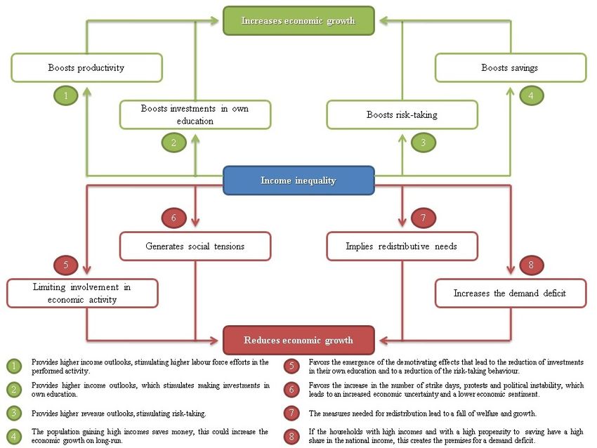
FigureFigure
1. The1.relationship
The relationship between
between income
income inequalityand
inequality andeconomic
economic growth
growth(source: own
(source: processing
own using
processing information
using information
extracted from The Impact of Income Inequality on Economic Growth [19]).
extracted from The Impact of Income Inequality on Economic Growth [19]).
Economic views are also divergent when studying the impact of economic growth
on income inequality. Maintaining its consistency, Kuznets claimed the existence of a
positive effect of economic growth on income inequality in low-income per capita states,Sustainability 2021, 13, 5204 4 of 16
Other studies have shown the existence of a negative relationship between income
inequality and economic growth. In this respect, Stiglitz concluded that income inequal-
ity slows down economic growth due to the reduced aggregate demand for low-income
individuals [28]. According to an OECD study, inequality diminishes people’s confi-
dence in markets and free trade, which may jeopardize long-term economic growth and
macroeconomic stability [29]. The analysis shows that high levels of income inequality
reduce confidence in national governments and institutions, and diminish the political
space for implementing reforms, which undermines the economic growth potential. Of
course, inequality may adversely impact growth through the channel of social or politi-
cal instability [5], but in most cases, its impact becomes visible in a couple of years [30].
Generally, the studied literature supports the hypothesis that income inequality is harmful
to economic growth, especially when it is perceived as unjust and insurmountable by the
population [31].
Shin confirmed the negative impact of inequality on growth in countries with low
development levels and proved its positive effects in the case of countries in advanced
development stages [3]. The negative effect of income inequality on economic growth
remained valid when Vo et al. examined the middle-income countries by applying a
GMM model on 86 middle-income countries [32], but also when Kim applied a GMM
and a fixed effects model on 40 OECD countries during the period 2004–2011 [33]. Other
authors supported the conclusion that the effect of income inequality on economic growth
varies according to the level of development, however, their findings were limited to
the negative relationship between the mentioned variables [34]. The study also shows
that in high-income countries, there is no significant correlation between inequality and
economic growth, given that opportunities are equally distributed, however, redistribution
through taxes and social transfers is beneficial for growth in underdeveloped countries
and unfavourable in developed countries. The same authors indicated (in another study)
that increasing inequality is detrimental to growth since it affects investment and the share
of the educated population but also increases the fertility rate [35]. The literature in this
field also confirms that high levels of income inequality are associated with periods of
slowing economic growth [36]. Other authors stated larger income gaps are associated with
an increase in the short-term economic growth, and therefore with a long-term slowing
down [4].
Economic views are also divergent when studying the impact of economic growth
on income inequality. Maintaining its consistency, Kuznets claimed the existence of a
positive effect of economic growth on income inequality in low-income per capita states,
and accordingly, a negative effect in the later stages of development [11]. This conclusion
has been also supported by other researchers [37–39], however, it was rejected by Sayed and
Ping, who confirmed an “N” shape of the long run relationship between income inequality
and economic growth [40], the Kuznets curve being the most important theory proving the
existence of this effect.
Bahmani-Oskooee and Gelan assessed the impact of economic growth on the distri-
bution of income in the US economy and found that, in the short run, economic growth
is associated with increased income inequality, while in the long run, the impact is nega-
tive [41]. There were also other studies focused on assessing the long run growth effect
on inequality in the US (covering the 1945–2004 period and using a PMG model) [42],
which confirmed that high growth volatility is positively linked with income inequality. In
fact, they concluded that the impact of growth volatility on inequality is only significant
when the economic growth rate is positive. However, other studies show that there is no
well-defined relationship between economic growth and income inequality [43,44]. This
finding was also supported by Thewissen, but the author demonstrated a positive effect of
top income shares on economic growth [45].
Following the examination of the economic literature, we found strong evidence
proving that the relationship between income inequality and economic growth was positive
in EU developed countries and negative in EU developing countries. Strong evidence fromSustainability 2021, 13, 5204 5 of 16
the economic literature confirming this hypothesis also implies that starting a discussion
on the way forward, but this should be focused on the case of EU developing countries,
since their situation is more challenging and vulnerable. The first recommendation consists
of improving the quality of institutions [46], but this is the most difficult one to implement
as a consequence of the resistance to a change in the parties benefiting from the exclusive
institutions. It is worth mentioning that this orientation is extremely wide and could imply
many reforms in several fields, including the improvement of labour market institutions.
Many authors stated that the engagement of countries to reduce inequality should start
with the identification process of vulnerable groups in the labour market [47], as well as
with the human development process based on better educational systems [48]. Remaining
connected to the topic of this paper, we found that the minimum inclusion income or
its reform is extremely used as a recommendation for developing countries by several
international bodies, including the ones representing the EU (e.g., European Commission).
The idea of ensuring a minimum inclusion income, unique or not, at the European
level, is a formula of real identity of the European model, an adaptive model in its evolution
to global developments as regards economic and social needs. In fact, the concern to ensure
a minimum inclusion income is both an expression of the relatively recent concerns of
creating a harmonious economic space developed throughout the European Union and
another formula that seeks to eliminate the effects of social injustice.
Arguments for standardizing the value of a minimum income are often political, and
for this reason, discussing these issues becomes not only appropriate but also necessary.
The targeted effects of a minimum income for inclusion are mainly of a social nature,
ensuring a decent standard of living for all citizens of the European Union. The fact that
the word “decent” is not a scientific term, but one that defines a social convention, makes
it impossible to investigate the final impact of introducing a minimum inclusion income,
unique for the whole geographical area of the EU. The economic effects of minimum income
compared to social assistance measures are at least debatable [49], while the beneficial
effects in the field of labour are not contested by economic theory.
Regarding the literature gaps, an unexplored effect in the quantitative assessment
of this paper is that exerted by the quality of institutions on the relationship between
income inequality and economic growth. This may be good orientation for our further
work. In addition, omitting other factors such as intergenerational mobility, inequality of
opportunity may generate misspecification in the assessment process. However, including
such factors in a model may raise additional issues as a consequence of the endogeneity
risk or of the difficulty in measuring such indicators. Moreover, the literature focuses
strictly on the Gini coefficient as a proxy for income inequality, and more emphasis should
be placed on other measures of income inequality (such as the Theil index, the Atkinson
index, the Palma ratio).
3. Materials and Methods
Through this section, we described the methodology framework used to assess the
relationship between income inequality and growth. The statistical data were extracted
from the Eurostat database covering the period 2010–2018 (yearly data) for EU-28 [50]. The
reason for using this time period was that we focused on the post-2009 economic shock
period, since the integration of pre-crisis data in the dataset may be theoretically wrong
and could facilitate spurious results of the regression as the crisis led to a structural change
in the economy and society. Even if a distinct assessment of the pre-crisis period would
have been beneficial, we limited our study to the post-2009 economic shock period taking
into consideration the low availability of data for Croatia. Moreover, we used EU-28 data,
since Brexit took effect in 2019, while the time period used in this study is 2010–2018.
First, we computed two clusters using the average GDP per capita expressed in the
purchasing power, standard over the period 2010–2018, to derive the level of development.
In this context, the EU-28 countries registering a GDP per capita (PPS) below the median of
this criterion were categorized in the group of developing EU Member States, while theSustainability 2021, 13, 5204 6 of 16
cluster of developed EU Member States was composed of the countries which registered
higher values of this indicator than the median. To verify whether the level of development
exercises an effect on the relationship between income inequality and growth, we estimated
an econometric model using the same methodology for each cluster. The statistical data
used were reported in Table 1.
Table 1. Data used (source: own processing).
Indicator Unit Source
Current prices, purchasing power standard
Gross domestic product—cluster criteria Eurostat
per capita
Chain linked volumes, percentage change on
Gross domestic product Eurostat
previous period (economic growth)
Scale from 0 to 100, 0 representing the lowest
Gini coefficient after social transfers Eurostat
dimension of income inequality and 100 the highest
Harmonized index of consumer prices (HICP) Annual average rate of change (inflation rate) Eurostat
Chain linked volumes, percentage change on
Gross capital formation Eurostat
previous period
High-tech exports The share of high-tech exports in total exports Eurostat
Employment rate of people graduating tertiary Employment rate of people ending their tertiary
Eurostat
studies in the last years education studies 1–3 years ago (20–34)
The structure of the model was decided according to the stationarity results we
obtained with the summary technique, which provides a broader view of the main results
of the relevant tests for stationarity, as (i) Levin, Lin and Chu t*; (ii) the Breitung t-stat;
(iii) Im, Pesaran and Shin W-stat; (iv) ADF—Fisher Chi-square; and (v) the PP—Fisher
Chi-square. The mentioned tests were performed using the Schwarz information criterion
for selecting the appropriate lag. Since the variables used proved to be stationary at level
and first difference, we decided to follow a classical approach by including in the model the
first difference of the variables stationary at I(1) and the current data series for the variables
stationary at level. We made these transformations to work with stationary variables since
this approach provides better results and reduces the likelihood of encountering issues
related to autocorrelation between residuals. In addition, we added some lags in the model,
according to the economic theory, to better catch the effects that are usually transmitted
over a period of 1 year.
Following the stationarity checking process, we used the redundant fixed effects–
likelihood ratio test to check the compatibility with a fixed effects model (FEM) or a random
effects model (REM), the results recommending the use of an FEM. In this context, we
applied the estimated generalized least squares method with fixed effects in Eviews 9.0.0.0
software—which was also reinforced by the cross-section weights option and White cross-
section covariance (tools used to increase the consistency of the estimators and to restrict
the existence of heteroskedasticity to low dimensions—cross-section SUR, another option
that addresses the heteroskedasticity issues, is not appropriate for models with a number
of cross-sections which is higher than the number of observations per cross-section)—on
Equation (1):
growthit = α0 + α1 ∆gini_t − 1it + α2 in f lation_t − 1it + α3 gc f changeit + α4 ∆hightechexportsit + α5 ∆tertemplrate13it + ε t (1)
where:
growth is economic growth, ∆gini_t − 1 represents the first difference of Gini coeffi-
cient lagged by one year, in f lation_t − 1 reflects the annual average rate of inflation lagged
by one year, gc f change is the percentage change of gross capital formation to catch the
impact of investments on growth, ∆hightechexports reflects the first difference of the high-
tech exports share in total exports and ∆tertemplrate13 refers to the first difference of theSustainability 2021, 13, 5204 7 of 16
employment rate of people ending their tertiary education studies 1–3 years ago (20–34 age
group). In addition, ε t represents the residuals, while α0 , ..., α5 are the impact coefficients.
Then, in line with the fixed effects model (FEM) features, we added 13 dummy vari-
ables in the initial equation to enhance the estimation (FEM literature indicates adding a
number of dummy variables equivalent to the number of cross-sections—1), as Equation (2):
growthit = β 0 + β 1 ∆gini_t − 1it + β 2 in f lation_t − 1it + β 3 gc f changeit + β 4 ∆hightechexportsit + β 5 ∆tertemplrate13it + ρ1 dummy1 + . . . + ρ13 dummy13 + µt (2)
where ρ1 , ..., ρ13 represents the intercepts of the dummies, β 0 , ..., β 5 are the new coefficients
and µt is the new residuals series.
Furthermore, we checked the Gauss–Markov hypotheses related to the maximum
verisimilitude of the estimators. In this respect, we first verified the statistical validity of the
model using the Fisher test. The next series of hypotheses we checked were related to the
residuals. Initially, we analysed the distribution of the residuals using Jarque–Bera to check
whether these were normally distributed. Afterward, we examined the possibility of cross-
section dependence (which is not favourable to BLUE—best linear unbiased estimators)
using Breusch-Pagan LM, Pesaran scaled LM, bias-corrected scaled LM, Pesaran CD and
Friedman Chi-square tests. Then, we verified the absence of heteroskedasticity using the
Breusch–Pagan–Godfrey test, but this has been performed in Microsoft Office Excel 2016,
since this calculation is not available in Eviews 9.0—Panel window. In order to obtain the
probability of the test which confirms the hypothesis of homoskedasticity—to the detriment
of heteroskedasticity, we estimated Equation (3):
µtitˆ2 = λ0 + λ1 ∆gini_t − 1it + λ2 in f lation_t − 1it + λ3 gc f changeit + λ4 ∆hightechexportsit + λ5 ∆tertemplrate13it + zt (3)
where λ0 , . . . , λ5 are the coefficients of the equation, zt represents the residuals term, and
µtitˆ2 is the square of the residuals term obtained from Equation (2). Then, we used the
R-squared value from Equation (3), as Equation (4):
R − squared Equation (3) ∗ n (4)
where n = number of observations taken into consideration in Equation (3).
The probability of the test was calculated in Excel 2016, using Equation (5):
CH ISQ.DIST.RT (the result o f the Equation (4), d f ) (5)
where df = degrees of freedom which is equivalent to the number of exogenous variables,
excepting the constant = 5.
The last hypothesis related to the residuals we have tested is the absence of auto-
correlation between these. Eviews does not allow this calculation in the panel window.
Therefore, we estimated Equation (6):
µtit = θ0 + θ1 ∆gini_t − 1it + θ2 in f lation_t − 1it + θ3 gc f changeit + θ4 ∆hightechexportsit + θ5 ∆tertemplrate13it + θ6 µt−1it + vt (6)
To compute the Breusch–Pagan–Godfrey probability, we followed the same method
presented above, and in this context, we used the CHISQ.DIST.RT function with the follow-
ing arguments: (i) the R-squared of the equation, multiplied by the number of observations
used in this equation; (ii) df = the number of lagged residuals from Equation (6).
Furthermore, we used the Klein criterion to verify the existence of multicollinearity,
which is rejected if the Pearson correlation between the exogenous variables is lower than
the R-squared obtained in Equation (2). However, even if the maximum verisimilitude
hypotheses are validated, there is also a need to check the robustness of the estimation. In
this context, we tested the robustness hypothesis following an approach used in a study,
which tried to identify whether the final results were influenced by the inclusion of one
year or one country in the model [51]. Therefore, in line with their methodology, we
estimated one distinct model for each year that we excluded from the analysis covering
the period 2010–2018 (9 models for each cluster and 18 models in total). As we mentioned
above, we also followed the authors’ approach in estimating different models for eachSustainability 2021, 13, 5204 8 of 16
cross-section that we excluded from the analysis (14 models for each cluster and 28 in total).
In sum, we performed the robustness test by estimating 46 additional models (using the
same methodology we described above—estimated generalized least squares method with
fixed effects reinforced by the cross-section weights option and the White cross-section
covariance) to check whether the final estimators were influenced by some temporary or
geographical features and developments.
4. Results
In this section, we provide the main results of our study. First, we used the GDP per
capita expressed in the purchasing power standard to split the European Union into two
groups of countries catching different stages of development. In this context, one group
includes the developed EU Member States, while the other is formed by the developing
EU Member States. As can be seen in Table 2, ES, IT, MT, FR, UK, FI, BE, SE, DE, AT, DK,
NL, IE, and LU forms the Developed EU Member States cluster, while the Developing EU
Member States group is formed by the remaining EU countries.
Table 2. Cluster formation—gross domestic product per capita expressed in purchasing power standard (source: own
processing using Eurostat data).
Cluster Countries
Spain, Italy, Malta, France, United Kingdom, Finland, Belgium, Sweden,
Developed EU Member States
Germany, Austria, Denmark, Netherlands, Ireland, Luxembourg
Bulgaria, Croatia, Romania, Latvia, Greece, Hungary, Poland, Slovakia,
Developing EU Member States
Portugal, Lithuania, Estonia, Slovenia, Cyprus, Czechia
Subsequently, we estimated the impact of income inequality on growth in the case
of each cluster designed (Table 3) using EGLS with fixed effects, since this is the most
appropriate method according to the Redundant Fixed Effects—Likelihood ratio test, its
corresponding probabilities being lower than 5% (Table 4).
Table 3. Estimation results: 2010–2018 (source: calculations of the authors using Eviews 9.0).
Developed EU Member Developing EU Member
Variables States Model States Model
Dependent—Growth
Coefficient/Std. Error Coefficient/Std. Error
0.213 ** −0.332 **
∆gini_t-1
−0.091 −0.15
−0.587 *** −0.333 ***
inflation_t-1
−0.043 −0.056
0.111 *** 0.148 ***
gcfchange
−0.012 −0.012
0.159 *** 0.163 ***
∆hightechexports
−0.059 −0.06
0.077 *** 0.083 ***
∆tertemplrate13
−0.023 −0.018
2.692 *** 2.261 ***
Constant
−0.116 −0.13
R-squared 0.8821 0.8424
Prob(F-statistic) 0 0
Observations 98 98
Note: *** significant at 1%, ** significant at 5%; standard errors in parentheses.Sustainability 2021, 13, 5204 9 of 16
Table 4. Tests performed (source: calculations of the authors using Eviews 9.0 and Microsoft Office Excel 2016).
Developed EU Member Developing EU Member
Test Hypothesis Found
States Model (p) States Model (p)
Compatibility with Fixed Effects Model
Fixed effects model is
Redundant Fixed Effects Test 0.000 (p < 0.05) 0.000 (p < 0.05)
appropriate
Breusch–Pagan Serial Correlation Test
R-squared
0.024476 0.033354 -
(dependent variable: resid01)
Observations (n) 84 84 -
n*R-squared 2.055 2.801 -
Degrees of freedom 1 1 -
0.1516 0.0941
Prob. Breusch–Pagan No serial correlation
(p > 0.05) (p > 0.05)
Heteroskedasticity Test—Breusch–Pagan–Godfrey
R-squared
0.064894 0.035113 -
(dependent variable: resid01ˆ2)
Observations (n) 98 98 -
n*R-squared 6.359 3.441 -
Degrees of freedom 5 5 -
0.2728 0.6323
Prob. Breusch–Pagan–Godfrey Homoskedasticity
(p > 0.05) (p > 0.05)
Cross-Section Dependence Tests:
0.5704 0.0125 No CD (developed)/
Breusch–Pagan LM
(p > 0.05) (p < 0.05) CD (developing)
0.2069 0.1615
Pesaran scaled LM No CD (both clusters)
(p > 0.05) (p > 0.05)
0.0151 0.8155 CD (developed)/
Bias-corrected scaled LM No CD (developing)
(p < 0.05) (p > 0.05)
0.2134 0.3847
Pesaran CD No CD (both clusters)
(p > 0.05) (p > 0.05)
0.0786 0.0797
Friedman Chi-square No CD (both clusters)
(p > 0.05) (p > 0.05)
Normality of Residuals Test
Prob. Jarque–Bera 0.750 (p > 0.05) 0.684 (p > 0.05) Normal distribution
We found that income inequality has a positive impact on growth in developed EU
countries, but it is also detrimental to growth in developing EU countries. According to the
results, an increase in the first difference of the Gini coefficient lagged by one year with one
deviation point leads to a hike in the economic growth equivalent to 0.21 percentage points
in developed EU countries. Conversely, we estimated a negative effect on growth of −0.33
percentage points. At first sight, our results may seem strange, but these are in line with
the literature review in this field, since in developed EU countries, income inequalities are
mostly generated by risk-taking behaviour and the greater implication of some individuals
in economic activity, which are also favourable to growth. On the other hand, in developing
EU Member States, income inequality has a negative impact on economic growth, since
these kinds of countries generally have low-quality institutions which promote welfare
losses, providing benefits to the elite or to restrained interest groups.
In addition, the tax systems from developed EU countries have a high level of pro-
gressivity, which reduces the income gap between individuals while limiting economic
growth, since the increase in tax rates slows down the economic growth rate. This argument
confirms a positive effect of income inequality on economic growth. On the other hand,Sustainability 2021, 13, 5204 10 of 16
some developing EU countries still use the flat tax rate and are more open to modify the
labour force or consumption taxes. As a consequence, the progressivity of tax systems may
not neutralize the effect of some fiscal policies that generally affect the socially vulnerable
groups, which increases the dimension of income inequality and lowers the economic
growth rate.
We enhanced our estimation by adding some control variables, such as the inflation
rate, the percentage change of gross capital formation, the share of high-tech exports in
total exports and the employment rate of people ending their tertiary education studies
1–3 years ago (20–34).
Considering the impact of prices, we found that an increase in the inflation rate of
the previous year by one percentage point has led to a fall in the current economic growth
by −0.33 percentage points in developing EU Member States. The negative effect is in
line with the economic theory since the increase in prices reduces the aggregate demand,
which also is detrimental to growth. Even if, from the perspective of aggregate supply, the
increase in prices may also generate additional revenues at the corporate level, the effect
could be reversed at a different point in time since the low demand may affect the aggregate
supply. In addition, inflation also affects economic growth through the uncertainty channel.
In the case of developed EU Member States, we found a higher impact (−0.58 percent-
age points) than the one mentioned above. The main reason arguing this impact difference
consists in the fact that the capacity of uncertainty to impact the economic sentiment is
greater in developed EU countries, which stands at the core of the Economic and Monetary
Union, these being more stable in terms of inflation. In addition, a shock in the evolution
of inflation could increase the perception of risks, as linkages in the Euro Area are more
prominent than the ones between the non-Euro Area Member States. Theoretically, non-
Euro Area Member States need to prove their macroeconomic stability before accessing the
Euro Area, but usually, these are the top of EU countries recording high inflation rates. It
is worth mentioning that only four non-EA countries registered an annual inflation rate
below 2% in 2019 (European Central Bank target), while 14 EA Member States were in line
with the ECB target. In this context, the investors and consumers are expecting stable price
developments, but this aspect increases the vulnerability of growth to price developments
when a shock occurs. From another point of view, price changes at the level of the Eurozone
generate more uncertainty which makes people act according to these risks.
Furthermore, we found that an increase in the percentage change of gross capital
formation with one percentage point raises the economic growth by 0.11 percentage points
in developed EU countries. However, the impact is a little higher in the case of developing
EU Member States (0.14 percentage points), which indicates a greater multiplier effect of
investments on growth in that group of countries.
On the other hand, we demonstrated that an increase in the first difference of the
share of high-tech exports in total exports with one percentage point has a positive impact
on growth of 0.16 percentage points in developing EU Member States, which is higher
than the one we found in developed EU countries (0.15 percentage points). This effect
is easy to argue since technological progress is one of the factors that enhances growth
potential. However, the impact difference is quite low, but our results indicate an additional
reason for Developing EU countries to engage in high-tech activities to support growth
and resilience.
We also estimated the impact of the tertiary employment rate on economic growth.
As Table 3 indicates, we found that an increase in the first difference of employment rate
of people ending their tertiary education studies 1–3 years ago (aged between 20–34)
with one percentage point enhances the economic growth with 0.08 percentage points
in developing EU Member States and 0.07 percentage points in developed EU countries.
Tertiary education is more correlated with growth than other levels of education, such as
primary or secondary education, whilst also being a significant driver of potential growth
and human development. Nevertheless, there are no significant differences between
the coefficients.Sustainability 2021, 13, 5204 11 of 16
In sum, our results show that all coefficients are statistically significant at 1%, except
the Gini coefficient which is significant at 5% in each model. The results also show that the
selected independent variables explain 84.24% (developing EU Member States) and 88.21%
(developed EU countries) of the evolution of the dependent variable, the high values of
R-squared also proving that we properly selected the explanatory variables. Moreover,
the models we estimated are statistically valid since the probabilities of the Fisher test are
lower than the significance threshold (5%).
To verify the hypothesis of the maximum verisimilitude of the estimators, we per-
formed additional tests related to the residuals (Table 4). First, we confirmed the hypotheses
of no serial correlation and homoskedasticity since their corresponding tests (Breusch–
Pagan and Breusch–Pagan–Godfrey) indicate probabilities higher than 5% for both models.
We then used five tests (Breusch–Pagan LM, Pesaran scaled LM, bias-corrected scaled
LM, Pesaran CD, and Friedman Chi-square) to check the dependence between cross-
sections. According to the results obtained, four of the five tests confirmed the null
hypothesis stating that there is no dependence between cross-sections in both cases; this
result is supported to a greater extent.
Finally, in Table 4, we provided the result of the Jarque–Bera test, which proves that
residuals are normally distributed, this being the last required criterion for confirming
the maximum verisimilitude hypothesis. This confirms that the estimators were prop-
erly selected and the results are robust, which supports high confidence in the obtained
impact coefficients.
Regarding the robustness testing, we presented the results of the 44 models performed
to check this hypothesis (Appendices A and B). Following this estimation, it is clear that
there are no significant large-scale differences between the results obtained in the 28 models
where we have run one separate model for each country excluded and the ones we obtain
in the baseline model. This confirms that the relationships between variables from the
baseline model were not placed on a different path as a consequence of some national
specificities or developments. However, when we gradually removed one year from the
analysis, in most cases, the results proved to be similar to the ones of the baseline model,
but we found two exceptions, these being related to the years 2012 and 2015. In 2015,
the coefficient of the share of high-tech exports in total exports (developed EU Member
States cluster) had a different sign compared to the one from the baseline model, but
this difference may be ignored as the coefficient became insignificant when this year was
extracted. Nevertheless, when 2012 is removed, there are three coefficients that change
their sign: the share of high-tech exports in total exports and inflation rate (developing EU
Member States cluster), respectively, the employment rate of people ending their tertiary
education studies 1–3 years ago (developed EU Member States).
Theoretically, this raises the possibility that the final results are influenced by the
2012 data. However, we took a look into the details of both clusters, and we found the
presence of autocorrelation when we removed the 2012 data (Breusch–Pagan test: 0.038
prob.—developing EU Member States; 0.005 prob.—developed EU Member States), which
confirms that we cannot trust these results, since the coefficients obtained in the model
without 2012 data are spurious. In addition, removing one year in separate models until all
years are removed may not be a useful approach in this case, as the estimated coefficient
covariance matrix becomes of reduced rank. Taking into consideration all the arguments
provided, we are confirming the robustness and verisimilitude of the results, the main
finding being related to the justification of a negative relationship between inequality and
growth in the case of developing EU Member States and a positive one in the case of
developed EU Member States.
5. Conclusions
Our paper shows that income inequality impacts economic growth differently, de-
pending on the country’s level of development. In this context, we found a positive impact
of income inequality on growth in the developed EU Member States. On the other hand,Sustainability 2021, 13, 5204 12 of 16
the relationship between income inequality and economic growth proved to be negative in
the case of developing EU Member States. This can be explained by the fact that income
inequalities are mostly generated by risk-taking behaviour and the greater implication of
some individuals in economic activity in developed EU countries (which is also favourable
to growth) while developing EU countries are associated with low-quality institutions
which extract wealth from the population and provide benefits to the elite or restrained
interest groups. Low-quality institutions are detrimental to growth since these lower the
economic expectations of individuals.
In addition, the tax systems of developed EU countries have a high level of progres-
sivity, which reduces the income gap between individuals while limiting the economic
growth since the increase in tax rates slows down the economic growth rate. This argument
confirms a positive effect of income inequality on economic growth. On the other hand,
some developing EU countries still use the flat tax rate and are more open to modify the
labour force or consumption taxes. As a consequence, the progressivity of tax systems may
not neutralize the effect of some fiscal policies that generally affect the socially vulnerable
groups, which increases the dimension of income inequality and lowers the economic
growth rate.
This provides important evidence for the need to promote an optimal level of income
inequality, which shall be in line with its social supportability. The main policy recommen-
dations are related to the improvement of institutions’ quality and the establishment of a
minimum inclusion income, which may facilitate the achievement of the social inclusion
objectives and increase the level of sustainable development. However, we did not test
the relationship between income inequality and growth in the long run, our findings and
results being limited to short run interpretation.
The analysis was enhanced by using other control variables for growth. Our results
show that there are no differences between the signs of the impact coefficients of the
independent variables (excepting the Gini coefficient) on growth obtained for each model.
In this respect, we found a negative relationship between economic growth and the inflation
rate lagged by one year, and a negative one between the dependent variable and the
percentage change of gross capital formation, and thus also for the high-tech exports
share in total exports. In addition, we also confirmed a positive relationship between
the employment rate of people ending their tertiary education studies 1–3 years ago and
economic growth in both models. Finally, following the methodology used, we confirmed
the robustness of the results and the maximum verisimilitude of the estimators.
However, there are some limitations regarding the interpretation of the results since
we estimated a unique impact of the income inequality on economic growth for each
development cluster. In this context, the impact coefficients are valid only when the full
country-group composition is examined. Identifying individual coefficients at the country
level is not the subject of this study since our work attempted to determine whether the
national level of development may change the sign of the relationship between income
inequality and economic growth. Nevertheless, studying individual country effects may
bring a value-added in our further work. Another limitation consists in the fact that there
is too much focus on income inequality measured through the Gini coefficient, and more
progress may be made in our further work by taking into consideration other indicators
catching the level of income inequality (such as Theil index, Atkinson index, Palma ratio).
Author Contributions: Conceptualization, M.D.; methodology, I.J.; software, I.J.; validation, M.D.
and D.H.; formal analysis, I.J. and D.H.; investigation, D.H. and A.B.; resources, A.B.; data curation,
I.J.; writing—original draft preparation, I.J. and D.H.; writing—review and editing, A.B.; visualization,
A.B.; supervision, M.D.; project administration, M.D. All authors have read and agreed to the
published version of the manuscript.
Funding: This research received no external funding.
Institutional Review Board Statement: Not applicable.
Informed Consent Statement: Not applicable.Sustainability 2021, 13, 5204 13 of 16
Data Availability Statement: Data are contained within the article but are also available on request.
Conflicts of Interest: The authors declare no conflict of interest.
Appendix A
Table A1. Robustness check—excluding one year, dependent: Gini (source: calculations of the authors using Eviews 9.0).
Variables
Year Excluded
∆gini_t-1 inflation_t-1 gcfchange ∆hightechexports ∆tertemplrate13 R-Squared
Developed EU Member States Model
0.211 * −0.558 *** 0.100 *** 0.110 * 0.042
2010 0.873
(0.110) (0.091) (0.007) (0.060) (0.025)
0.223 *** −0.337 *** 0.090 *** 0.146 *** 0.070 **
2011 0.896
(0.081) (0.092) (0.005) (0.044) (0.034)
0.237 *** −0.255 *** 0.095 *** 0.161 *** −0.018 **
2012 0.969
(0.063) (0.025) (0.002) (0.020) (0.007)
0.238 −0.828 *** 0.028 ** 0.120 0.188 ***
2013 0.799
(0.263) (0.117) (0.013) (0.155) (0.048)
0.078 −0.837 *** 0.018 ** 0.113 0.146 ***
2014 0.894
(0.055) (0.059) (0.008) (0.124) (0.024)
0.393 *** −0.744 *** 0.043 *** −0.189 0.139 **
2015 0.844
(0.081) (0.046) (0.015) (0.122) (0.051)
0.367 *** −0.292 *** 0.191 *** 0.366 0.059 ***
2016 0.919
(0.120) (0.050) (0.013) (0.310) (0.018)
0.155 * −0.492 *** 0.139 *** 0.146 0.051 **
2017 0.907
(0.078) (0.060) (0.012) (0.157) (0.024)
0.231 *** −0.576 *** 0.127 *** 0.199 *** 0.075 **
2018 0.894
(0.067) (0.044) (0.011) (0.029) (0.029)
Developing EU Member States Model
−0.124 −0.368 *** 0.147 *** 0.090 0.064 ***
2010 0.796
(0.106) (0.069) (0.012) (0.061) (0.015)
−0.207 −0.093 0.121 *** 0.193 *** 0.026
2011 0.720
(0.135) (0.161) (0.013) (0.066) (0.018)
−0.037 0.202 ** 0.078 *** −0.072 ** 0.041
2012 0.821
(0.083) (0.098) (0.006) (0.032) (0.040)
−0.459 *** −0.173 *** 0.171 *** 0.208 *** 0.121 ***
2013 0.931
(0.089) (0.030 (0.004) (0.059) (0.018)
−0.577 *** −0.199 *** 0.182 *** 0.033 0.090 ***
2014 0.948
(0.099) (0.061) (0.012) (0.092) (0.010)
−0.636 *** −0.259 *** 0.183 *** 0.033 0.029 **
2015 0.950
(0.024) (0.043) (0.008) (0.052) (0.014)
−0.300 ** −0.469 *** 0.119 *** 0.186 *** 0.074 ***
2016 0.931
(0.144) (0.052) (0.003) (0.037) (0.011)
−0.177 −0.383 *** 0.128 *** 0.211 *** 0.076 ***
2017 0.870
(0.226) (0.038) (0.011) (0.078) (0.014)
−0.267 * −0.397 *** 0.137 *** 0.151 ** 0.077 ***
2018 0.873
(0.148) (0.041) (0.014) (0.059) (0.012)
Note: *** significant at 1%; ** significant at 5%; * significant at 10%; standard errors in parentheses.Sustainability 2021, 13, 5204 14 of 16
Appendix B
Table A2. Robustness check—excluding one country, dependent: Gini (source: calculations of the authors using Eviews 9.0).
Country Variables
Excluded ∆gini_t-1 inflation_t-1 gcfchange ∆hightechexports∆tertemplrate13 R-Squared
Developed EU Member States Model
BE
0.220 *** −0.632 *** 0.111 *** 0.166 *** 0.078 ***
0.890
(0.082) (0.041) (0.012) (0.061) (0.022)
DK 0.241 ** −0.570 *** 0.111 *** 0.178 *** 0.085 *** 0.885
(0.091) (0.046) (0.013) (0.064) (0.032)
DE 0.196 * −0.580 *** 0.115 *** 0.167 ** 0.080 *** 0.887
(0.106) (0.049) (0.018) (0.063) (0.020)
IE 0.081 −0.502 *** 0.110 *** 0.069 0.089 *** 0.854
(0.074) (0.052) (0.017) (0.072) (0.017)
ES
0.215 ** −0.569 *** 0.107 *** 0.153 *** 0.065 ***
0.886
(0.101) (0.042) (0.012) (0.056) (0.020)
FR 0.213 * −0.632 *** 0.109 *** 0.168 ** 0.059 ** 0.886
(0.123) (0.045) (0.013) (0.064) (0.029)
IT 0.242 ** −0.622 *** 0.105 *** 0.159 ** 0.110 *** 0.862
(0.100) (0.047) (0.011) (0.062) (0.027)
LU 0.290 *** −0.593 *** 0.112 *** 0.186 ** 0.074 *** 0.894
(0.109) (0.054) (0.017) (0.071) (0.023)
MT
0.137 ** −0.487 *** 0.135 *** 0.044 0.060 ***
0.835
(0.068) (0.047) (0.005) (0.088) (0.021)
NL 0.277 *** −0.583 *** 0.122 *** 0.203 *** 0.073 *** 0.892
(0.083) (0.045) (0.012) (0.068) (0.024)
AT 0.229 ** −0.596 *** 0.110 *** 0.173 *** 0.081 *** 0.888
(0.100) (0.044) (0.012) (0.048) (0.024)
FI 0.219 ** −0.546 *** 0.108 *** 0.152 ** 0.089 *** 0.880
(0.085) (0.046) (0.013) (0.058) (0.028)
SE
0.161 −0.603 *** 0.101 *** 0.129 ** 0.074 ***
0.888
(0.110) (0.044) (0.011) (0.061) (0.021)
UK 0.313 *** −0.640 *** 0.109 *** 0.189 *** 0.081 *** 0.892
(0.102) (0.045) (0.013) (0.054) (0.081)
Developing EU Member States Model
BG
−0.363 ** −0.302 *** 0.144 *** 0.176 *** 0.117 ***
0.857
(0.152) (0.069) (0.013) (0.060) (0.027)
CZ −0.347 ** −0.322 *** 0.144 *** 0.145 ** 0.076 *** 0.841
(0.150) (0.059) (0.015) (0.070) (0.020)
EE −0.332 ** −0.341 *** 0.159 *** 0.170 ** 0.047 * 0.849
(0.150) (0.072) (0.015) (0.070) (0.026)
EL −0.318 ** −0.333 *** 0.145 *** 0.146 ** 0.078 *** 0.818
(0.152) (0.051) (0.012) (0.061) (0.017)
HR
−0.341 ** −0.306 *** 0.140 *** 0.163 ** 0.107 ***
0.844
(0.150) (0.063) (0.012) (0.064) (0.017)
CY −0.326 ** −0.333 *** 0.144 *** 0.122 0.064 *** 0.824
(0.161) (0.056) (0.016) (0.094) (0.013)
LV −0.326 ** −0.367 *** 0.150 *** 0.157 *** 0.078 *** 0.852
(0.145) (0.054) (0.012) (0.059) (0.017)
LT −0.283* −0.358 *** 0.159 *** 0.176 *** 0.073 *** 0.862
(0.147) (0.050) (0.008) (0.059) (0.015)
HU
−0.283 *** −0.326 *** 0.137 *** 0.116 * 0.096 ***
0.826
(0.106) (0.072) (0.014) (0.065) (0.021)
PL −0.313 ** −0.345 *** 0.151 *** 0.177 *** 0.088 *** 0.848
(0.150) (0.058) (0.013) (0.057) (0.019)
PT
−0.330 ** −0.338 *** 0.141 *** 0.159 ** 0.071 ***
0.803
(0.157) (0.058) (0.013) (0.064) (0.020)
RO −0.378 ** −0.356 *** 0.150 *** 0.196 *** 0.091 *** 0.843
(0.180) (0.065) (0.010) (0.070) (0.019)
SI −0.340 ** −0.318 *** 0.144 *** 0.165 *** 0.091 *** 0.845
(0.153) (0.056) (0.013) (0.059) (0.016)
SK −0.340 ** −0.343 *** 0.152 *** 0.164 *** 0.088 *** 0.858
(0.147) (0.053) (0.012) (0.047) (0.018)
Note: *** significant at 1%; ** significant at 5%; * significant at 10%; standard errors in parentheses.Sustainability 2021, 13, 5204 15 of 16
References
1. European Commission. Reflection Paper on the Deepening of the Economic and Monetary Union; European Commission: Brussels,
Belgium, 2017. Available online: https://ec.europa.eu/commission/publications/reflection-paper-deepening-economic-and-
monetary-union_en (accessed on 10 December 2020).
2. Bilan, Y.; Mishchuk, H.; Samoliuk, N.; Yurchyk, H. Impact of Income Distribution on Social and Economic Well-Being of the State.
Sustainability 2020, 12, 429. [CrossRef]
3. Shin, I. Income Inequality and Economic Growth. Econ. Model. 2012, 29, 2049–2057. [CrossRef]
4. Halter, D.; Oechslin, M.; Zweimüller, J. Inequality and Growth: The Neglected Time Dimension. J. Econ. Growth 2014, 19, 81–104.
[CrossRef]
5. Neves, P.C.; Silva, S.M.T. Survey Article—Inequality and Growth: Uncovering the Main Conclusions from the Empirics. J. Dev.
Stud. 2014, 50, 1–21. [CrossRef]
6. Policardo, L.; Punzo, L.F.; Sánchez Carrera, E.J. Brazil and China: Two Routes of Economic Development? Rev. Dev. Econ. 2016,
20, 651–669. [CrossRef]
7. Madsen, J.B.; Islam, M.R.; Doucouliagos, H. Inequality, Financial Development and Economic Growth in the OECD 1870–2011.
Eur. Econ. Gov. 2018, 101, 605–624. [CrossRef]
8. Brida, J.G.; Sánchez Carrera, E.J.; Segarra, V. Clustering and Regime Dynamics for Economic Growth and Income Inequality.
Struct. Chang. Econ. Dyn. 2019, 52, 99–108. [CrossRef]
9. Sakaki, S. Equality in Income and Sustainability in Economic Growth: Agent-Based Simulations on OECD Data. Sustainability
2019, 11, 5803. [CrossRef]
10. Seo, H.J.; Kim, H.S.; Lee, Y.S. The Dynamic Relationship between Inequality and Sustainable Economic Growth. Sustainability
2020, 12, 5740. [CrossRef]
11. Kuznets, S. Economic Growth and Income Inequality. Am. Econ. Rev. 1955, 45, 1–28.
12. Kaldor, N. A Model of Economic Growth. Econ. J. 1957, 67, 591–624. [CrossRef]
13. Okun, A.M. Equality and Efficiency: The Big Tradeoff ; The Brookings Institution: Washington, DC, USA, 1975.
14. Chletsos, M.; Fatouros, N. Does Income Inequality Matter for Economic Growth? An Empirical Investigation. 2016.
Available online: https://mpra.ub.uni-muenchen.de/id/eprint/75477 (accessed on 12 December 2020).
15. Huang, C.C.; Chang, J.J.; Hung, H.W. Progressive Tax and Inequality in a Unionized Economy. Scand. J. Econ. 2020, 122, 38–80.
[CrossRef]
16. Cornia, G.A.; Court, J. Inequality, Growth and Poverty in the Era of Liberalization and Globalization. Policy Brief 4 of the
UNU World Institute for Development Economics Research 2001. Available online: https://www.wider.unu.edu/publication/
inequality-growth-and-poverty-era-liberalization-and-globalization (accessed on 12 December 2020).
17. United Nations Development Programme. Humanity Divided: Confronting Inequality in Developing Countries; UNDP: New York,
NY, USA, 2013; Available online: https://www.undp.org/content/undp/en/home/librarypage/poverty-reduction/humanity-
divided--confronting-inequality-in-developing-countries.html (accessed on 10 December 2020).
18. Cho, D.; Kim, B.M.; Rhee, D.E. Inequality and Growth: Nonlinear Evidence from Heterogeneous Panel Data; Working Paper; Korea
Institute for International Economic Policy: Sejong, Korea, 2014; No. 14-01. [CrossRef]
19. Petersen, T.; Schoof, U. The Impact of Income Inequality on Economic Growth. Impulse 2015, 5, 1–12.
20. Henderson, D.J.; Qian, J.; Wang, L. The Inequality—Growth Plateau. Econ. Lett. 2015, 128, 17–20. [CrossRef]
21. Delbianco, F.; Dabús, C.; Caraballo, M.A. Income Inequality and Economic Growth: New Evidence from Latin America. Cuad.
Econ. 2014, 33, 381–398. [CrossRef]
22. Rubin, A.; Segal, D. The Effects of Economic Growth on Income Inequality In the US. J. Macroecon. 2015, 45, 258–273. [CrossRef]
23. Marrero, G.A.; Rodriguez, J.G. Inequality of Opportunity and Growth. J. Dev. Econ. 2013, 104, 107–122. [CrossRef]
24. Roemer, J.E.; Trannoy, A. Equality of Opportunity: Theory and Measurement. J. Econ. Lit. 2016, 54, 1288–1332. [CrossRef]
25. Marrero, G.A.; Rodriguez, J.G.; Van der Weide, R. Unequal Opportunity, Unequal Growth. Policy Res; Policy Research Working
Paper; World Bank: Washington, DC, USA, 2016; No. 7853. Available online: https://openknowledge.worldbank.org/handle/10
986/25298 (accessed on 14 December 2020).
26. Ayar, S.; Ebeke, C. Inequality of Opportunity, Inequality of Income and Economic Growth. World Dev. 2020, 136, 105115.
[CrossRef]
27. Bradbury, K.; Triest, R. Inequality of Opportunity and Aggregate Economic Performance. Russel Sage Found. J. Soc. Sc. 2016, 2,
178–201. [CrossRef]
28. Stiglitz, J.E. The Price of Inequality: How Today’s Divided Society Endangers Our Future; W. W. Norton: New York, NY, USA, 2012.
29. OECD. Opportunities for All: A Framework for Policy Action on Inclusive Growth; OECD Publishing: Paris, France, 2018; Available
online: http://www.oecd.org/economy/opportunities-for-all-9789264301665-en.htm (accessed on 15 December 2020).
30. Kennedy, T.; Smyth, R.; Valadkhani, A.; Chen, G. Does Income Inequality Hinder Economic Growth? New Evidence Australian
Taxation Statistics. Econ. Model. 2017, 65, 119–128. [CrossRef]
31. Mourao, P.; Junqueira, A. Through the Irregular Paths of Inequality: An Analysis of the Evolution of Socioeconomic Inequality in
Brazilian States Since 1976+. Sustainability 2021, 13, 2356. [CrossRef]
32. Vo, D.H.; Nguyen, T.C.; Tran, N.P.; Vo, A.T. What Factors Affect Income Inequality and Economic Growth in Middle-Income
Countries? J. Risk Financ. Manag. 2019, 12, 40. [CrossRef]You can also read