Resilient Ramp Control for Highways Facing Stochastic Perturbations
←
→
Page content transcription
If your browser does not render page correctly, please read the page content below
Resilient Ramp Control for Highways Facing
                                                      Stochastic Perturbations
arXiv:2104.10823v1 [math.OC] 22 Apr 2021

                                                                                                                                                  ∗†
                                                     Li Jin, Yu Tang, Alexander A. Kurzhanskiy and Saurabh Amin
                                                                                         April 23, 2021

                                                                                             Abstract
                                                        Highway capacity is subject to stochastic perturbations due to weather, traffic mix-
                                                    ture, driver behavior, etc. However, systematic approaches to traffic control with per-
                                                    formance guarantees in the face of such perturbations are still limited. In this paper,
                                                    we develop a novel control-theoretic method for designing perturbation-resilient ramp
                                                    metering. We consider a cell-transmission model with 1) Markovian cell capacities
                                                    and 2) buffers representing on-ramps and upstream mainline. Using this model, we
                                                    analyze the stability of on-ramp queues by constructing piecewise Lyapunov functions
                                                    motivated by the nonlinear traffic dynamics. Then, we design ramp controllers that
                                                    guarantee bounds for throughput and queue sizes. We formulate the coordinated ramp
                                                    metering problem as a bi-level optimization with non-convex inner problems. To ad-
                                                    dress the computational issue, we also consider a localized and a partially coordinated
                                                    reformulation. A case study of a 18.1-km highway in Los Angeles, USA indicates a
                                                    7.6% (resp. 8.8%) reduction of vehicle-hours-traveled obtained by the localized (resp.
                                                    partially coordinated) control, both outperforming the 5.4% reduction obtained by the
                                                    classical ALINEA policy.

                                                  Keywords: Markov processes, nonlinear systems, cell transmission model, traffic control.

                                              ∗
                                                  This work was in part supported by NYU Tandon School of Engineering, C2SMART University Trans-
                                           portation Center, US NSF Award CMMI-1949710 and CAREER Award CNS-1453126, SJTU UM Joint
                                           Institute, J. Wu & J. Sun Endowment Fund, and Singapore NRF Future Urban Mobility.
                                                †
                                                  L. Jin is with the UM Joint Institute and the School of Electronic Information and Electrical Engineering,
                                           Shanghai Jiao Tong University, China. L. Jin is also and Y. Tang is with the Tandon School of Engineering,
                                           New York University, USA. A. A, Kurzhanskiy is with the Institute of Transportation Studies, University
                                           of California, Berkeley, USA. S. Amin is with the Laboratory of Information and Decision Systems and the
                                           Department of Civil and Environmental Engineering, Massachusetts Institute of Technology, USA (emails:
                                           li.jin@sjtu.edu.cn, tangyu@nyu.edu, akurzhan@berkeley.edu, amins@mit.edu).

                                                                                                  1
1 Introduction
Advances in smart transportation provide opportunities for improving highway system perfor-
mance. Technologies such as embedded sensors and dynamic traffic signal controllers enable
highway control strategies including ramp metering, variable speed limit, and dynamic rout-
ing [1, 2, 3]. These methodologies have been extensively developed in deterministic settings.
However, transportation systems are subject to intrinsic uncertainties that can compromise
the deterministic approaches [4, 5]. One perturbation widely reported is highway capacity
fluctuation [6, 7], but limited results are available for highway control design in the face
of such perturbations. The following example shows that highway dynamics can be better
modeled with the consideration of stochastic capacities.
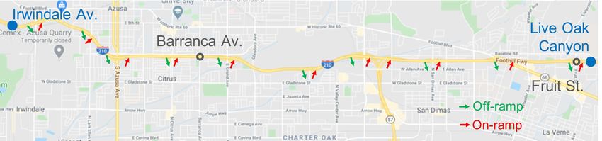
We consider a 18.1-km Interstate 210 Eastbound (I-210E) section as shown in Figure 1a.
We calibrate both a conventional cell-transmission model (CTM) and a stochastic-switching
cell transmission model (SS-CTM) with Markovian capacities using PeMS data [8]; see Ap-
pendix A for calibration details. The results imply significant capacity fluctuations near
Barranca Avenue and Fruit Street; see Figures 1b and 1c. We also simulated both calibrated
models and compared them in terms of mean absolute percentage error (MAPE) of vehicle
travel times.
(a) A section of I-210E.
8000 8000
Capacity subject to perturbation
Capacity (veh/h)
Capacity (veh/h)
7000 7000 Nominal capacity
6000 6000
5000 Capacity subject to perturbation 5000
Nominal capacity
4000 4000
12:00 15:00 18:00 21:00 12:00 15:00 18:00 21:00
(b) Barranca Av. (c) Fruit St.
Figure 1: Calibrated capacity fluctuation.
The conventional CTM gives a MAPE 8.9%, while the SS-CTM yields a MAPE of 4.3%.
Figure 2 visualizes the real and simulated density maps. The CTM underestimates the traffic
jam between Irwindale Avenue and Barranca Avenue, while the SS-CTM significantly reduces
this modeling error by introducing stochastic capacities. The result indicates that the control
design based on the CTM may fail to understand the congestion mechanism.
In this paper, we develop a control-theoretic approach to designing ramp control resilient
to the above-mentioned perturbations. The proposed approach can guarantee a lower bound
for throughput and an upper bound for queue sizes in the face of stochastic perturbations.
280 80 80
Fruit St. Fruit St. Fruit St.
Density(veh/(km · lane))
Density(veh/(km · lane))
Density(veh/(km · lane))
60 60 60
40 40 40
Barranca Av. Barranca Av. Barranca Av.
20 20 20
Irwindale Av. Irwindale Av. Irwindale Av.
0 0 0
12:00 15:00 18:00 21:00 12:00 15:00 18:00 21:00 12:00 15:00 18:00 21:00
(a) True data. (b) CTM. (c) SS-CTM.
Figure 2: Comparison of density maps.
To this end, we consider a spatially discretized traffic flow model with stochastic capacities.
This model extends the well-known cell-transmission model (CTM [9]) by introducing two
features: 1) highway capacities varying according to a Markov chain and 2) infinite-sized
buffers denoting on-ramps and upstream mainline. The model tracks mainline traffic densi-
ties, buffer queues, and time-variant cell capacities. Using this model, we study the stability
of buffer queues under a class of ramp metering policies. The stability results lead to a
bi-level, non-convex formulation of the coordinated control design problem (similar to those
in [10, 11]). To address the computational difficulty, we consider localized and partially
coordinated reformulations. The former relies only on local information (similar to those
in [12, 13]) and does not consider the interaction between multiple ramps, and the latter
sequentially determines the ramp controllers such that the upstream controllers depend on
the downstream ones. We apply both approaches to the above I-210 example and show how
they improve from ramp controllers obtained using deterministic methods.
Prior literature has investigated various ramp control schemes, mainly for deterministic
settings. Papageorgiou et al. proposed the integral controller ALINEA for localized ramp
metering [12] and then generalized it to the coordinated METALINE [10]. The efficacy of
these two algorithms were validated in a series of field tests [14] and prompted a bunch of
ALINEA-like controllers [13, 15, 16]. Although these emerging controllers have refined the
original ALINEA, they still rely on nominal critical density. Another way is to formulate
on-ramp control as mathematical programming based on deterministic traffic flow models.
Optimal ramp metering over a finite horizon was addressed offline via nonlinear optimization
[17, 18, 19, 20, 21]. Real-time ramp metering is also available through the technique of model
predictive control (MPC) [22, 23], but its implement in practice is hard due to costly compu-
tation. The distributed MPC-based ramp metering has been proposed to address this issue
[24, 25]. An alternative is to design optimal or near-optimal static state feedback controllers
with simple structures [26], which is considered in our paper. It does not require heavy real-
time computation and is flexible since ramp metering can be designed in either a centralized
or a decentralized manner. However, our previous work showed that capacity perturbations
may destabilize on-ramp queues that are stable in the deterministic, nominal/average setting
[5]. The main reason is that capacity perturbations can induce traffic queues and bottle-
necks that do not exist in the nominal setting and are thus not accounted for by nominally
3efficient controllers. This result indicates that the approaches built in deterministic settings
may behave poorly in the face of perturbations. Some attempts to solve this problem have
been reported in the literature. For example, dynamical estimation of critical density was
introduced into the classical ALINEA [27]. Besides, robust optimization has been introduced
into ramp metering; the methods were built on the uncertainty sets of demands and traffic
parameters [28, 29, 30, 31]. However, limited results are available for resilient ramp metering
against stochastic capacity perturbations in a systematical way.
This paper focuses on the following major challenges for control design in the stochastic
setting.
(i) How to formulate the stability constraint and the control cost (objective function)?
(ii) How to obtain control policies from highly complex optimization problems, where mul-
tiple ramp controllers are coupled?
We address (i) by exploiting the Foster-Lyapunov criterion [32]. This criterion leads to
the drift condition for the feedback-controlled SS-CTM, which is a sufficient stability condi-
tion. The generic form of the Foster-Lyapunov criterion requires verifying the drift condition
everywhere over the state space, but we simplify the stability constraint by constructing
invariant set, a subset of the state space, and showing that it suffices to verify the drift con-
dition over the invariant set. Second, if the drift condition holds, we can utilize it to obtain a
lower bound of throughput for a given control law and a upper bound of buffer queue size for
certain traffic demand along with a control law. In this paper, we consider designing control
laws that minimize the queue size for given traffic demands. Thus the upper bound is used
as a proxy for the exact queuing cost. The numerical examples in Sections 3 and 4 show that
this upper bound is a reasonable proxy.
To address (ii), we develop localized and partially coordinated reformulations of the gen-
eral coordinated control design problem. The reformulations compromise control efficiency
but reduce computational complexity. The localized ramp metering is designed independently
of other ramp controllers. For this reformulation, we propose a Lyapunov function motivated
by the insights into traffic dynamics, which simplifies the stability condition (Theorem 1)
and the control objective. Then the controller can be obtained by solving a bi-level program-
ming with a non-convex inner problem, where the decision variables of the outer problem are
control parameters and the decision variables of the inner problem are traffic densities and
queue lengths. The technique of localized reformulation can also be applied to the fully coor-
dinated control design (Theorem 2), which inspires the partially coordinated reformulation.
The fully coordinated design is aware of the mutual interactions among ramp controllers,
while the partially coordinated approach only considers the impacts of downstream ramp
metering on the upstream ones. Briefly, the partially coordinated control design decomposes
the coordination problem into a set of interconnected sub-problems and solves them one by
one from the downstream to the upstream. We also present the stability condition of this
approach (Theorem 3) and use the numerical example in Section 4 to show that it can yield
a good approximate solution.
We validate the proposed approach in the I-210E case study introduced in Figure 1a.
Two benchmarks are considered, one without ramp metering and the other controlled by the
state-of-the-practice ALINEA. The evaluation of different scenarios shows that, compared
4to ALINEA, the proposed methods are more efficient in terms of reducing total vehicle
hours (both on the mainline and at the on-ramps). The proposed localized and partially
coordinated control design reduced total vehicle hours by 7.6% and 8.8% respectively, while
ALINEA contributed a reduction of 5.4%. It should be pointed out that the result does not
imply that our proposed method will substitute for the classical ramp control policies such
as ALINEA but only indicates that the classical methods can be further refined in stochastic
environment.
The rest of this paper is organized as follows. We first introduce the SS-CTM and
formulate the control problem in Section 2. The following Sections 3 and 4 focus on localized
and coordinated ramp metering, respectively. Then, Section 5 presents a case study of our
methods. Finally, we summarize the paper and discuss the future research in Section 6.
2 Modeling and formulation
In this section, we introduce the stochastic switching cell-transmission model (SS-CTM) and
formulate the control problem.
2.1 Stochastic traffic model
We consider a highway with K mainline cells, K on-ramp buffers, and K − 1 off-ramps, as
shown in Figure 3. Note that the first buffer is not an actual on-ramp; instead, it represents
the upstream highway section and stores the upstream queue. Each cell k has the following
parameters: length lk (km), free-flow speed vk (km/hr), congestion wave speed wk (km/hr)
and jam density njamk (veh/km). The kth buffer has a capacity Uk (veh/hr). Every on-ramp
k is subject to a constant demand αk ∈ [0, Uk ]. The continuous state of the highway is (q, n),
0))1*-234
'())"*$% !"##$% !"##$& !"##$+ !"##$!"% !"##$!
!! #! #" #$
,-./#./" Q1 (t) N1 (t) N 2 (t) N 3 (t) N K!1 (t) N K (t)
"! "" "# "$
'())"*$& '())"*$+ '())"*$!
0/1*-234 !" !# Q (t) !$
Q2 (t) 3 QK (t)
Figure 3: A highway with K cells, K buffers and K − 1 off-ramps.
where q = [q1 , · · · , qK ]T is the vector of buffer queues and n = [n1 , · · · , nK ]T is the vector of
traffic densities in mainline cells. The set of permissible queue lengths is Q := RK ≥0 , and the
QK jam
set of traffic densities is N := k=1 [0, nk ]. Hence, the continuous state space is Q × N .
In our traffic flow model, the cell capacities stochastically vary over time according to a
finite-state Markov process over a set of modes denoted by S = {1, · · · , m}. The inter-mode
transition rates are {λs,s′ ; s, s′ ∈ S}. Without loss of generality, we let λs,s = 0 for all s ∈ S.
Hence, we have
Pr{S(t + δ) = s′ |S(t) = s} = λs,s′ δ + o(δ),
where δ is an infinitesimal time increment. Every mode s is associated with a vector of cell
capacities [F1,s , · · · , FK,s]T . Let S(t) be the mode at time t. We assume that the Markov
5chain governing the mode transition process {S(t); t ≥ 0} admits with a unique vector of
steady-state probabilities p = [p1 , · · · , pm ]T such that
X X
ps′ λs′ ,s = ps λs,s′ , s ∈ S, (1a)
s′ ∈S s′ ∈S
X
ps = 1, (1b)
s∈S
ps ≥ 0, s ∈ S. (1c)
For each k, we also define
X
F̄k := ps Fk,s , Fkmax := max Fk,s , Fkmin := min Fk,s ,
s∈S s∈S
s∈S
which can be interpreted as the mean, the maximal, and the minimal capacity of cell k,
respectively. We recognize Fkmax as the nominal capacity of cell k and define the critical
density as
F max
nck := k .
vk
Following [9], we assume that the critical density nck is characterized by
vk nck ≤ wk (njam
k − nck ), (2)
which implies the receiving flow is not less than the sending flow at the critical density nck .
For notational convenience, we use φ = (s, q, n) to denote hybrid state and Φ(t) =
(S(t), Q(t), N(t)) to denote hybrid stochastic process. Note that the process belongs to
piecewise deterministic Markov process. Following this convention, we let Qk (t) be the queue
length in the kth buffer and Nk (t) denote the traffic density in the kth cell at time t, and
thus Q(t) = [Q1 (t), · · · , QK (t)]T ∈ Q and N(t) = [N1 (t), · · · , NK (t)]T ∈ N .
Next, we specify the flow functions and traffic dynamics. For k = 1, · · · , K − 1, let
βk ∈ (0, 1] denote the fixed mainline ratio, i.e. the fraction of traffic from cell k entering cell
k + 1; the remaining traffic flow leaves the highway at the kth off-ramp. Naturally, we let
βK := 0. Thus, the outflow fk from cell k is given by
n 1 o
fk (φ) = min vk nk , Fk,s, wk+1 (njam
k+1 − nk+1 ) − r (q
k+1 k+1 , nk+1 ) , k ≤ K − 1, (3a)
βk
fK (φ) = min{vK nK , FK,s}, (3b)
where rk is the on-ramp flow from on-ramp k to cell k, given by
(
min{αk , wk (njam
k − nk )} qk = 0,
rk (qk , nk ) = jam k = 1, · · · , K. (4)
min{Uk , wk (nk − nk )} qk > 0,
In addition, we define
max{k1 ,k2 }−1
Y
γk1 ,k2 := βj , 1 ≤ k1 , k2 ≤ K, k1 6= k2 , (5)
j=min{k1 ,k2 }
6where γk1 ,k2 denotes the fraction of traffic flows from cell min{k1 , k2} entering cell max{k1 , k2 }.
For convenience, we also define γk,k := 1 for k = 1, . . . , K.
We further consider that on-ramp flows are regulated by affine controllers. This control
law is favored because the simple state feedback can achieve performance comparable to that
of other methods such as model predictive control [33]. It should be noted that our methods
do not necessarily require the affine structure, which implies the generalization for nonlinear
state feedback. Specifically, the control law (ramp metering policy) µ : N → RK−1 ≥0 is given
by
µk (nk ) = uk − κk nk , k = 2, . . . , K, (6)
where the controller µk parameterized by uk and κk limits the ramp flow based on the traffic
density nk . It indicates monotonicity that µk (nk ) decreases as the downstream traffic density
nk increases. The proposed ramp metering (6) relies on local measurements, like the integral
controller ALINEA, but the control parameters uk and κk can be optimized in either a
localized or a coordinated manner. The optimal values of these control parameters rely on
the problem settings, such as traffic demand and capacity fluctuation. For example, when
mainline demand increases, the designed ramp metering tends to be more aggressive with
smaller uk or larger κk .
Then, the controlled on-ramp flow rkµ is rewritten as
rkµ (qk , nk ) = min{rk (qk , nk ), µk (nk )}, k = 2, · · · , K. (7)
With a slight abuse of notation, we use fkµ : S × Q × N → R≥0 , Qµ (t) ∈ Q and N µ (t) ∈ N
to denote the outflow from cell k, buffer queues and traffic densities under the control law µ,
respectively. Thus, the dynamics of the buffer queues Qµ (t) and traffic densities N µ (t) can
be written as follows:
Q̇µ (t) = Gµ (S(t), Q(t), N(t)), (8a)
Ṅ µ (t) = H µ (S(t), Q(t), N(t)), (8b)
where Gµ : S × Q × N →K and H µ : S × Q × N →K are vector fields defined as
Gµ1 (φ) := α1 − r1 (q1 , n1 ), (9a)
µ µ
H1 (φ) := r1 (q1 , n1 ) − f1 (φ) /l1 , (9b)
Gµk (φ) := αk − rkµ (qk , nk ), k = 2, . . . , K, (9c)
µ µ µ µ
Hk (φ) := βk−1 fk−1 (φ) + rk (qk , nk ) − fk (φ) /lk , k = 2, . . . , K. (9d)
One can show that Gµ and H µ are continuous and bounded and that Qµ (t) and N µ (t) are
continuous in time t [5].
Finally, we present the density boundaries of invariant sets used for control design. For
some set S × X ⊆ S × Q × N , we say n∗k is a lower bound (resp. upper bound) of density nk
over S × X if Hkµ (φ) ≥ 0 (resp. Hkµ (φ) ≤ 0) for any φ ∈ {(s, q, n)|(s, q, n) ∈ S × X , nk = n∗k }.
7We define
min{α1 , F1max }
n1 := , (10a)
v1
min
min{βk−1 min{vk−1 nk−1, Fk−1 } + αk , Fkmax }
nk := , k = 2, · · · , K, (10b)
vk
min{U1 , F1max }
n
✿1
:= , (10c)
v1
µ F max
n
✿k
:= min{νkµ , k }, k = 2, · · · , K, (10d)
vk
Fkmin
n̄k :=njam
k − , k = K, · · · , 1, (10e)
wk
jam
min{Fkmin , minnk+1 ∈[nk+1 ,ñµk+1 ] (wk+1(njam µ
k+1 − nk+1 ) − rk+1 (1, nk+1 ))/βk }
ñµk :=nk − , k ≤ K − 1,
wk
(10f)
where νkµ is the unique solution of βk−1 min{vk−1 nk−1 , Fk−1
min
} + rkµ (1, νkµ ) = vk νkµ because of the
monotonicity of µ. (10a)-(10b) denote the lower bound of nk if there is no queue in buffer k,
while (10c)-(10d) mean the lower bound of nk if buffer k has queuing flows. (10e) represents
the upper bound of nk if cell k is free from downstream congestion, while (10f) indicates the
upper bound of nk if the outflow from cell k is affected by downstream congestion. Note
that the superscript µ indicates the dependency of boundaries on the control law µ. For the
µ
convenience of notation, we also define n ✿1
:= n
✿1
and ñµK := n̄K .
2.2 Problem formulation
Our control objective is to stabilize and enhance highway system performance in the face
of capacity perturbation. For performance metric under a control law µ, we consider time-
average queue size Q̄µ in the buffers (on-ramps and upstream mainline). This quantity
benefits stability analysis over an infinite horizon. Besides, it is related with practical perfor-
mance measurement vehicle hours traveled [11, 14]. Thus it can serve as an objective function
of our control design.
We first consider the following notion of stability: the buffer queues are stable if there
exists Z < ∞ such that for each initial condition φ(0) ∈ S × Q × N ,
t K
1
Z hX i
lim sup E Qµk (τ ) dτ ≤ Z, (11)
t→∞ t τ =0 k=1
where Qµk (τ ) denotes the queue size in the k-th buffer under the control law µ. Practically, this
stability indicates that the time-average queue length in all buffers are bounded regardless
of the initial condition. For stable buffer queues, the time-average queue size Q̄µ is given by
t K
1
Z X
lim Qµk (τ ) dτ = Q̄µ a.s. (12)
t→∞ t τ =0 k=1
8We present the original problem formulation P0 as follows:
(P0 ) min Q̄µ
µ
s.t. every buffer queue is bounded on average. (13)
In the following, we apply the Foster-Lyapunov criterion to rewriting the formulation P0
mathematically. The criterion presents a sufficient condition for (11) and is stated below:
Foster-Lyapunov criterion [32]. Consider a Markov process X(t) with state space X and
infinitesimal generator L . If there exists a Lyapunov function V : X → R≥0 and constants
c > 0, d < ∞ satisfying
L V (x) ≤ −cg(x) + d, ∀x ∈ X , (14)
then for each initial condition x ∈ X
t
1 d
Z
lim sup E[g(X(t))]dτ ≤ . (15)
t→∞ t τ =0 c
We term (14) drift condition. In our problem, we have
X
L V (φ) = Gµ (φ)T ∇q V (φ) + H µ (φ)T ∇n V (φ) + λss′ (V (s′ , q, n) − V (φ)) (16)
s′ ∈S
for any Lyapunov function V : S × Q × N → R≥0 by noting that the traffic model SS-CTM
belongs to piecewise deterministic Markov process [5, 34].
The criterion above essentially states that g(X(t)) is bounded on average with an upper
boundary d/c if the drift condition (14) holds for g. Usually, g has a physical meaning. For
our problem, we let g(φ) = K
P
k=1 k denote the sum of buffer queue sizes. Hence the Foster-
q
Lyapunov criterion can be used to derive an upper bound for mean buffer size. Besides,
L V (φ) given by (16) is related to traffic demands. Intuitively, the drift condition does not
hold given large traffic demands. We define mainline throughput under certain control law
as the maximum mainline demand that maintains the stability. Thus we can obtain a lower
bound of mainline throughput by increasing the mainline demand until the drift condition
(14) fails.
It should be pointed out that we do not need to verify the drift condition (14) over
S × Q × N as the SS-CTM is piecewise deterministic Markov process. Instead, we only need
to consider initial conditions in an invariant set Mµ ⊆ Q × N [35], where the superscript µ
to indicate the dependency of Mµ on µ. An invariant set Mµ is a closed set such that for
each initial condition φ ∈ S × Mµ ,
(Q(t), N(t)) ∈ Mµ , ∀t ≥ 0.
Since it is hard to compute Q̄µ analytically, we propose choosing the upper bound dµ /cµ
of Q̄µ as the control objective. So given a invariant set Mµ and a Lyapunov function V :
9S × Mµ → R≥0 , the problem P0 is approximated as follows:
dµ
(P1 ) min
µ µ
µ;c ,d ∈R>0 cµ
X
s.t. Gµ (φ)T ∇q V (φ) + H µ (φ)T ∇n V (φ) + λs,s′ (V (s′ , q, n) − V (φ))
s′ ∈S
K
X
≤ −cµ qk + dµ , ∀φ = (s, q, n) ∈ S × Mµ , (17)
k=1
where the constraint (17) ensures that the drift condition (14) holds. The programming P1
simultaneously provides multiple ramp metering, which is recognized as a formulation of the
coordinated control design. It in general leads to a sub-optimal control µ to the original
problem P0 , since the upper bound dµ /cµ is a proxy for the mean queue length Q̄µ .
Directly solving P1 is still challenging. First, the objective function is non-convex and the
constraint (17) can be also non-convex for a general Lyapunov function V (φ). Besides, the
constraint (17) is infinite dimensional by noting the continuous state (q, n) ∈ Mµ . To address
the control design, we first consider localized ramp metering in Section 3 and reformulate P1
as a bi-level programming that can be solved quickly. Then we consider coordinated ramp
metering in Section 4 and provide a bi-level programming as well. For the large-scale coor-
dinated control, we present a partially coordinated approach that decomposes the problem
into a series of sub-problems. This approach can efficiently yield near-optimal solutions to
the fully coordinated control design.
3 Localized control design
In this section, we discuss the design of localized ramp metering that addresses a highway
bottleneck illustrated by Figure 4. The bottleneck is modeled as a two-cell highway section
where cells 1&2 (mainline) and buffer 2 (on-ramp) make up a typical merging area and buffer
1 represents the upstream highway. Cells 1 and 2 are congested due to merging conflicts and
capacity perturbations. We assume that the outflow from cell 2 discharges with free-flow
speed, which indicates that the traffic congestion of cells 1 and 2 is independent of their
downstream traffic. The control action we consider is to regulate the flow from buffer 2 to
cell 2. This ramp metering is localized in that i) it only relies on local information of buffers
1&2 and cells 1&2, and ii) it is designed independently of other ramp meters.
/))0*,12
'())"*$% !"##$% !"##$&
!!
+,-.#-." Q1 (t) N1 (t) N 2 (t)
'())"*$&
/.0*,12 !"
Q2 (t)
Figure 4: Two-cell highway section.
10Our approach consists of two steps: finding a set of stabilizing controllers and determining
the optimal stabilizing controller. Thus we first develop a criterion for checking whether a
localized controller µlo is stabilizing. To state this result, we consider the set Mµlo :=
∪i1 ,i2 ∈{0,1} Mµi1lo,i2 with (q1 , q2 , n1 , n2 ) ∈ Mµi1lo,i2 := Qµ1,ilo1 × Qµ2,ilo2 × N1,i
µlo
1
µlo
× N2,i 2
where i1 (resp.
i2 ) indicates whether there is queue in buffer 1 (resp. buffer 2) and we define
µlo
Qµ1,0lo × N1,0 µlo
:= {0} × [n1 , ñµ1 lo ], Qµ1,1lo × N1,1 := R>0 × [n
✿1
, ñµ1 lo ],
Qµ2,0lo × N2,0
µlo
:= {0} × [n2 , n̄2 ], Qµ2,1lo × N2,1
µlo
:= R>0 × [nµlo
✿2
, n̄2 ].
The following lemma states that Mµlo is an invariant set, which is proved in Appendix B.
Lemma 1 The set Mµlo is an invariant set for the two-cell highway section.
We also define the sets E1µlo and E2µlo :
(q2 , n1 , n2 ) ∈ E1µlo :=({0} × {n
✿1
} × [n2 , n̄2 ]) ∪ ({1} × {n
✿1
} × [n
✿2
µlo
, n̄2 ]),
(q2 , n1 , n2 ) ∈ E2µlo :={1} × {n1 } × [n
✿2
µlo
, n̄2 ].
Our results will show that the localized control design only needs to consider E1µlo and E2µlo ,
instead of Mµlo , by exploiting the properties of traffic dynamics.
µlo
Besides, define Dk,s (X ) for s ∈ S and k ∈ {1, 2} as
µlo
Dk,s (X ) := max γ1,k Gµ1 lo (φ) + γ1,k l1 H1µlo (φ) + γ2,k Gµ2 lo (φ) + γ2,k ρ2 (n2 )l2 H2µlo (φ), (18)
(q,n)∈X
where the weight ρ2 (n2 ) quantifies the impacts of H2µlo (φ). Essentially, Dk,s µlo
(X ) can be
recognized as the maximum net outflow from cell k in mode s under the control law µlo . We
n −n
let ρ2 (n2 ) := n̄22 −n2 for the convenience of analysis if the congestion of cell 2 will hamper
2
the outflow from cell 1. This weight indicates H2µlo (φ) has more influence on the net outflow
when the traffic density n2 is higher. But if cells 1 and 2 are decoupled by the control law
µlo such that
w2 (njam
2 − n2 ) − r2µlo (1, n2 ) ≥ β1 F1max , ∀n2 ∈ [n2 , n̄2 ], (19)
the outflow from cell 1 will not be impeded by cell 2. In that case, we do not need to
distinguish the impacts of different n2 and can let ρ2 (n2 ) := 1.
With the definitions above, we state the main result of this section:
Theorem 1 Consider the two-cell highway model with a ramp controller µlo . Then, the
highway model is stable if
nX X o
µlo µlo µlo µlo µlo
D̄ := max ps D1,s (E1 ), ps D2,s (E2 ) < 0, (20)
s∈S s∈S
where ps are the solutions to (1a)-(1c). Furthermore, if (20) holds, the on-ramp queues are
upper-bounded by
1 t d
Z
lim sup E[|Q1 (τ ) + Q2 (τ )|]dτ ≤ , (21)
t→∞ t τ =0 −D̄ µlo
where d ∈ (0, ∞) is a constant independent of µlo .
11We term D̄ µlo mean drift. Hence, the above result can be stated as follows: the two-cell
system is stable and the buffer queue size is bounded on average if the mean drift is negative.
µlo
With the physical meaning of Dk,s (X ), the negative mean drift also means that the expected
net outflow of cells 1 and 2 are both less than zero.
In the following, we present the controller design based on the stability criterion. Because
d is independent of µlo , minimizing the upper bound −d/D̄ µlo is equivalent to minimizing the
mean drift D̄ µlo . It suggests that the objective function of P1 can be replaced by D̄ µlo . Note
that minimizing negative D̄ µlo can also be interpreted as minimizing the negative expected
net outflows of cells 1 and 2. In general cases, cells 1 and 2 are coupled. Thus, by letting
n −n
ρ2 (n2 ) = n̄22 −n2 , we formulate the design of localized ramp metering as follows:
2
(P2 ) min D̄ µlo
u2 ,κ2 ∈R>0
D̄ µlo ∈RCorollary 1 Consider the two-cell highway section decoupled by a control law µlo satisfying
U1 ≥ F1max , (23a)
β1 F1min + r2µlo (0, nc2 ) ≥ F2max , (23b)
β1 α1 + r2µlo (1, nc2 ) ≥ F2max . (23c)
Then, the highway model is stable if and only if
α1 < F̄1 , (24a)
β1 α1 + α2 < F̄2 . (24b)
In the rest of this section, we first illustrate the stability condition and the localized
control design with a numerical example. Then, we provide the proofs of Theorem 1 and
Corollary 1.
3.1 Numerical example
Consider a highway section (see Figure 4) with the parameters in Table 1, where the capacity
of cell 2 switches between 3000 veh/hr and 6000 veh/hr and the transition rates λ1,2 and λ2,1
have the magnitude similar to the practical values in Table 5.
Table 1: Model parameters.
Parameter Notation Value Unit
Free-flow speed v1 , v2 100 km/hr
Congestion-wave speed w1 , w2 25 km/hr
Jam density njam
1 , n2
jam
200, 300 veh/km
Mainline ratio β1 0.75 -
F1,1 F2,1 4000 6000
Two-mode mainline capacity veh/hr
F1,2 F2,2 4000 3000
Transition rate λ1,2 , λ2,1 0.9 /hr
On-ramp capacity U1 , U2 4000, 1200 veh/hr
Demand α1 , α2 3500, 600 veh/hr
We first computed the mean drift D̄ µlo for various values of u2 and κ2 , which is presented
in Figure 5a. Theorem 1 outlines the stable regime with negative D̄ µlo . Since this theorem
only states the sufficient condition for stability, it is unknown whether the regime with non-
negative D̄ µlo is stable. But the result adequately shows that (κ∗2 , u∗2 ) = (4750, 25) minimizes
D̄ µlo and can be recognized as the solution to the programming P2 . We also simulated the
model numerically and obtained the average value of the total queue length
T
1 X µlo
Q̂µlo = q̂1 (t) + q̂2µlo (t) ,
T t=1
where T denotes the number of simulation steps and q̂kµlo (t) denotes the queue size in buffer
k at time step t for k = 1, 2. The simulated value Q̂µlo serves as an approximation of time-
average value Q̄µlo given by (12). It was found that (κ†2 , u†2 ) = (4750, 24) minimizes Q̂µlo
13-80
200
Simulated queue size Q̂µlo (veh)
Simulated queue size Q̂µlo (veh)
200
-100
Parameter u2 (veh/h) 1000 400
-100
180 180
Mean drift (veh/h)
Mean drift (veh/h)
Mean drift (veh/h)
300
2000 unknown -120
stable -120
200 160 160
3000
100 -140
-140
4000 140 140
(κ†2, u†2) (κ∗2, u∗2) 0
5000 -160 -160
-100 120 120
6000 -200
0 10 20 30 40 50 -180 -180
100 100
Parameter κ2 (km/h)
3000 4000 5000 6000 0 10 20 30 40 50
Parameter u2 (veh/h) Parameter κ2 (km/h)
(a) D̄ µlo under various (b) D̄ µlo and Q̂µlo under fixed (c) D̄ µlo and Q̂µlo under fixed
(κ2 , u2 ). κ2 . u2 .
Figure 5: Mean drift D̄ µlo and simulated queue size Q̂µlo .
and can be seen as the solution to the programming P0 . Clearly, the example demonstrates
that the programming P2 can provide good approximate solutions for P0 . The rationale lies
in that to minimize D̄ µlo is essentially to minimize −d/D̄ µlo , the upper bound of Q̄µlo . We
further illustrated the correspondence between D̄ µlo and Q̂µlo by fixing one control parameter
and tuning the other. Figure 5b shows the case where κ2 is fixed as 25 km/h and u2 ranges
between 2500 veh/h and 6000 veh/h, and Figure 5c presents the other case where u2 equals
4750 veh/h and κ2 varies from 0 km/h to 50 km/h. It is reasonable to find that too small or
too large parameters lead to undesirable queue sizes. For example, tight ramp metering with
small u2 will increase the on-ramp queue size; loose ramp metering with large u2 will yield the
control input µlo,2 (n2 ) always larger than on-ramp flow r2 (q2 , n2 ) and will not decrease the
queue size in the upstream mainline. Figures 5b and 5c demonstrate that this law applies
to D̄ µlo as well. It indicates that we can find appropriate control parameters by minimizing
D̄ µlo instead of directly minimizing Q̄µlo .
We also explore the impacts of demands on the control design. Figure 6a presents the
relationship between the parameter u2 and the mainline demand α1 given the on-ramp de-
mand α2 = 600 veh/h and the parameter κ2 = 25 km/h; Figure 6b presents the relationship
between the parameter κ2 and the mainline demand α1 given the on-ramp demand α2 = 600
veh/h and the parameter u2 = 4750 veh/h. It is shown that u2 tends to decrease and κ2
tends to increase when α1 increases. This finding indicates that our control design yields
sensible controllers that further restrict on-ramp flows if the mainline congestion worsens.
Next, we compare the proposed method with the classical control ALINEA that regulates
on-ramp flows µk (t) via the following feedback:
µk (t) = µk (t − 1) − KR (nk (t) − nck ), (25)
where KR is the control gain, nk (t) is the traffic density of cell k at time step t and nck is
the critical density of cell k. Note that ALINEA is essentially an integral controller and the
empirical results suggested that the gain KR equals 40 (km·lane)/h [13]. Figure 7a illustrates
the comparison given different mainline demands α1 . It is not surprising to find that both
ALINEA and our method contribute to the marginal reduction of queue sizes when α1 is
145000 5000
Parameter u2 (veh/h)
Parameter u2 (veh/h)
4900 4900
4800 4800
4700 4700
4600 4600
4500 4500
3300 3400 3500 3600 3700 3300 3400 3500 3600 3700
Mainline demand α1 (veh/h) Mainline demand α1 (veh/h)
(a) Impacts on u2 . (b) Impacts on κ2 .
Figure 6: Impacts of demands on control parameters.
low. But the ramp metering begins to work as the increasing mainline demand brings about
long queues. In that case, our method can outperform ALINEA in terms of shortening the
queues. Figure 7b shows the other comparison given various F2,2 . Here we use σ(F2,s ),
standard deviation of F2,s , to quantify the capacity fluctuation. We observed the phenomena
similar to those in Figure 7a. The result indicates that our method is more efficient than
ALINEA in face of intense capacity fluctuation.
(a) Impacts of α1 . (b) Impacts of F2,2 .
Figure 7: Control comparison.
3.2 Proof of Theorem 1
To prove the result, we construct a Lyapunov function for the stochastic traffic model and
show that (20) ensures the Foster-Lyapunov criterion for stability. Consider the invariant set
Mµlo and the Lyapunov function
2 1 n2
1
X Z
V (φ) := qk γ1,k q1 + γ2,k q2 + γ1,k l1 n1 + γ2,k l2 ρ2 (ξ)dξ + bk,s , φ ∈ S × Mµlo (26)
k=1
2 2 n2
where the parameters bk,s ≥ 0 are solutions to
µlo
X X
Dk,s (Ekµlo ) + λs,s′ (bk,s′ − bk,s ) = µlo
ps Dk,s µlo
′ (Ek ), s ∈ S, k ∈ {1, 2}.
s′ ∈S s′ ∈S
The existence of bk,s is guaranteed by Lemma 2 proved in Appendix C.
15Lemma 2 The system of equations (27), given a set of zk,s , has a non-negative solution for
bk,s . X X
zk,s + λs,s′ (bk,s′ − bk,s ) = ps zk,s′ , s ∈ S, k = {1, · · · , K}. (27)
s′ ∈S s′ ∈S
Applying the infinitesimal generator, we have
X2
L V (φ) = γ1,k Gµ1 lo (φ) + γ1,k l1 H1µlo (φ) + γ2,k Gµ2 lo (φ) + γ2,k ρ2 (n2 )l2 H2µlo (φ)
k=1
X 2
X Z n2
µlo
+ λs,s′ (bk,s′ − bk,s ) qk + Gk (φ)(γ1,k n1 + γ2,k ρ2 (ξ)dξ + bk,s ).
s′ ∈S k=1 n2
The rest of this proof is devoted to verifying the drift condition
L V (φ) ≤ −cµlo (q1 + q2 ) + d, ∀φ ∈ S × Mµlo
for some cµlo > 0 and d < ∞. We consider Mµlo by discussing whether there are queues in
both buffer 1 and 2.
3.2.1 Mµ0,0lo
Over this set, we have q1 = q2 = 0. Since Gµ1 lo (φ), Gµ2 lo (φ), n2 , ρ2 (n2 ) are all bounded, there
exists d1 < ∞ such that L V (φ) ≤ d1 , ∀φ ∈ S × Qµ1,0lo × Qµ2,0lo × N1,0 µlo µlo
× N2,0 .
3.2.2 Mµ1,0lo ∪ Mµ0,1lo ∪ Mµ1,1lo
Over the set S × (Mµ1,0lo ∪ Mµ0,1lo ∪ Mµ1,1lo ), we have
µlo µlo µlo µlo µlo µlo µlo
D1,s (M1,0 ∪ M1,1 )q1 ≥ G1 (φ) + l1 H1 (φ) + β1 G2 (φ) + β1 ρ2 (n2 )l2 H2 (φ) q1 ,
µlo
D2,s (Mµ0,1lo ∪ Mµ1,1lo )q2 ≥ β1 Gµ1 lo (φ) + β1 l1 H1µlo (φ) + Gµ2 lo (φ) + ρ2 (n2 )l2 H2µlo (φ) q2 .
µlo
Next, we show D1,s (Mµ0,1lo ∪ Mµ1,1lo ) = D1,s
µlo
(E1µlo ). Combining (9a)-(9d) and yields
µlo
D1,s (Mµ1,0lo ∪ Mµ1,1lo ) = maxµ α1 + β1 α2 − (1 − β12 ρ2 (n2 ))f1µlo (φ)
(q,n)∈M1 lo
− β1 (1 − ρ2 (n2 ))r2µlo (φ) − β1 ρ2 (n2 )f2µlo (φ) .
µlo
Note that q1 is cancelled and that D1,s (Mµ1,0lo ∪ Mµ1,1lo ) is monotonically decreasing in n1 . So
µlo
we reduce D1,s µlo
(Mµ1,0lo ∪ Mµ1,1lo ) to D1,s (E1µlo ). Similarly, we can show D2,s µlo
(Mµ0,1lo ∪ Mµ1,1lo ) =
µlo µlo
D2,s (E2 ). Therefore we have
2
X X
µlo
L V (φ) ≤ Dk,s (Ekµlo ) + λ s,s′ (b
k,s′ − bk,s ) qk + d2
k=1 s′ ∈S
X µlo
≤ max ps Dk,s (Ekµlo )(q1 + q2 ) + d2 , ∀φ ∈ S × (Mµ1,0lo ∪ Mµ0,1lo ∪ Mµ1,1lo )
k∈{1,2}
s∈S
where d2 ≤ ∞. Hence, there exists cµlo := −D̄ µlo > 0.
Combining the results above, we conclude that the drift condition (14) is achieved with
c = −D̄ µlo and d = max{d1 , d2 }, which implies the stability.
µlo
163.3 Proof of Corollary 1
We first consider the necessity. If the two-cell highway section is stable, we must conclude
the time-average inflow is less than the time-average outflow, which indicates (24a)-(24b).
Then, we show the sufficiency. Consider the set M̃µlo := ∪i1 ,i2 ∈{0,1} M̃µi1lo,i2 with M̃µi1lo,i2 :=
µlo
Q̃µ1,ilo1 ,i2 × Q̃µ2,ilo1 ,i2 × Ñ1,i 1 ,i2
µlo
× Ñ2,i 1 ,i2
where
( (
{0} ik = 0 [nk , n̄k ] ij = 0, ∀1 ≤ j ≤ k
Q̃µk,ilo1 ,i2 := µlo
, Ñk,i 1 ,i2
:= , k = 1, 2.
R>0 ik = 1 [nck , n̄k ] otherwise
M̃µlo is an invariant set as stated in Lemma 3 that is proved in Appendix D.
Lemma 3 The set M̃µlo is an invariant set for the two-cell highway section satisfying (19)
and (23a)-(23c).
Note that M̃µlo is in general tighter than Mµlo and leads to tighter E˜1µlo := {0}×{nc1 }×[nc2 , n̄2 ]
and E˜2µlo := {1} × {n1 } × [nc2 , n̄2 ].
µlo ˜µlo µlo
According to Theorem 1, we only need to consider D1,s (E1 ) and D2,s (Ẽ2µlo ). Noting
ρ2 (n2 ) = 1 in case of the decoupled cells 1 and 2, we have
µlo
D1,s (Ẽ1µlo ) = max µ
(1 − β12 )(α1 − min{v1 n1 , F1,s }) + β1 (β1 α1 + α2 − min{v2 n2 , F2,s })
(q2 ,n1 ,n2 )∈Ẽ1 lo
=(1 − β12 )(α1 − F1,s ) + β1 (β1 α1 + α2 − F2,s ).
µlo ˜µlo
Similarly, we obtain D2,s (E2 ) = β1 α1 +α2 −F2,s . So given (24a)-(24b), the stability condition
(20) is satisfied.
4 Fully/partially coordinated control design
Indeed, one can apply the localized control design to independently producing ramp metering
for each on-ramp. This approach does not consider the influence of downstream congestion.
However, on-ramps are usually located closely in practice, and traffic jam easily spills back
and blocks the upstream on-ramps. To address this shortcoming, we propose the partially
coordinated control design that sequentially determines ramp meters from the downstream
to the upstream. This manner helps the controllers consider their downstream bottlenecks
and ramp metering polices. Before presenting the partial coordination, we first introduce
the fully coordinated control design that simultaneously designs multiple ramp controllers.
It motivates the partially coordinated reformulation.
We assume the fully coordinated ramp metering µfc applied to the K-cell highway shown
in Figure 3. To state the results, we consider the set Mµfc := ∪i1 ,···,iK ∈{0,1} Mµi1fc,···,iK with
(q1 , · · · , qK , n1 , · · · , nK ) ∈ Mµi1fc,···,iK = Qµ1,ifc1 × · · · × QµK,i
fc
K
× N1,i µfc
1
µfc
× · · · × NK,i K
where
[nk , ñµk fc ]
( (
µfc {0} ik = 0 µfc
ik = 0
Qk,ik := , Nk,ik := µfc µfc . (28)
R>0 ik = 1 [n✿k
, ñk ] ik = 1
The following lemma states that Mµfc is an invariant set, which is proved in Appendix E.
17Lemma 4 The set Mµfc is an invariant set for the K-cell highway section.
Besides, we define Ekµfc := {(q, n)|qk > 0, (q, n) ∈ Mµfc } and
XK
µfc µfc µfc µfc µfc
Dk,s (X ) := maxµ γ1,k G1 (φ) + l1 H1 (φ) + γj,k Gj (φ) + ρj (nj )lj Hj (φ) . (29)
(q,n)∈Ek fc
j=2
µfc µlo
Dk,s (X ) has the same physical meaning as Dk,s (X ) given by (18). Likewise, we let ρj (nj ) =
nj −nj
µ
ñ fc −n
if cell k impedes the outflow from cell k − 1. Otherwise, we let ρj (nj ) := 1.
j j
Below we state the stability condition of the fully coordinated ramp:
Theorem 2 Consider a K-cell highway with a control law µfc . Then, the highway model is
stable if
X µfc
D̄ µfc := max ps Dk,s (Ekµfc ) < 0, (30)
k=1,···,K
s∈S
where ps are the solutions to (1a)-(1c). Furthermore, if (30) holds, the buffer queues are
upper-bounded by
t K
1 d
Z hX i
lim sup E Qk (τ ) dτ ≤ , (31)
t→∞ t τ =0 k=1
−D̄ µfc
where d ∈ (0, ∞) is a constant independent of µfc .
According to Theorem 2, we can recast P1 as P3 presented below. The constraints (32)
n −n
are derived from plugging (9a)-(9d) into (30) with ρj (nj ) = ñµjfc −nj . Like the localized case
j j
P2 , the fully coordinated control design problem P3 belongs to bi-level programming with
non-convex lower-level optimization, where u, κ and D̄ µfc are the decision variables of the
outer problem, q and n are the decision variables of the inner problems. Solving P3 is more
challenging than solving P2 , since the decision variables in both the inner and outer problem
increase with the scale of highway stretch. Consequently, it is even harder to find the globally
optimal u and κ of P3 for large-scale cases.
(P3 ) min D̄ µfc
u,κ∈RK−1>0
D̄ µfcWe propose a partially coordinated approach to address the computational issue. The
partial coordination means that each ramp controller neglects its upstream highway and
only considers its downstream ramp metering. The design of the control law µpc follows the
procedure: we first design the controller µpc,K for ramp K, and then design the controller
µpc,K−1 for ramp K − 1 based on the controller µpc,K , and so forth until all K − 1 controllers
µ
are obtained. To state the mathematical formulation, we define the set Ek pc for k = 2, · · · , K
such that
µ
(qk , qk+1 , · · · , qK , nk−1 , nk , nk+1 , · · · , nK ) ∈ Ek pc
µpc µpc µpc µ µpc µ
[
= {1} × Qk+1,i k+1
× · · · × QK,i K
× {nk−1} × [n
✿k
, ñk pc ] × Nk+1,i k+1
× · · · × NK,ipcK ,
ik+1 ,···,iK ∈{0,1}
(33)
µ µ
where Qj,ipcj and Nj,ipcj for j = k + 1, · · · , K are defined in the same way as (28) with control-
µ µ µ
dependent boundaries n✿ j pc and ñj pc . For convenience, we also define E1 pc such that
µ
(q1 , q2 , · · · , qK , n1 , n2 , · · · , nK ) ∈ E1 pc
[ µ µpc µ µ µ
= {1} × Q2,ipc2 × · · · × QK,i K
× [n
✿1
, ñ1 pc ] × N2,ipc2 × · · · × NK,ipcK .
i2 ,···,iK ∈{0,1}
Then, solving Pk4 for k = K, · · · , 3, 2 produces the controller µpc,k . For certain Pk4 , the bound-
µ µpc µpc µpc
aries ñk pc , · · · , ñK−1 and n✿ k+1 ,···,n
✿K
are determined by the controllers µpc,k+1, · · · , µpc,K
pc µ
that have been addressed while n
✿k
relies on the controller µpc,k to be solved. Note that
the variable dimension of the outer problem in Pk4 have nothing to with the scale of highway
stretch. Thus we can solve them in the way of the localized control design.
µ
(Pk4 ) min D̄k pc
uk ,κk ∈R>0
µ
D̄k pcTheorem 3 Consider a K-cell highway section with a control law µpc . Then, the highway
model is stable if
µ µ
X
ps Dk,spc (Ek pc ) < 0, k = 1, 2, . . . , K, (35)
s∈S
where ps are the solutions to (1a)-(1c).
nj −nj
Note that plugging (9a)-(9d) into (35) with ρj (nj ) = µ
ñj pc −nj
leads to the constraints (34).
Furthermore, if the control law µpc decouples the highway such that
µ
wk+1 (njam pc max
k+1 − nk+1 ) − rk+1 (1, nk+1 ) ≥ βk Fk , ∀nk+1 ∈ [nk+1 , n̄k+1 ], k = 1, · · · , K − 1 (36)
and the traffic dynamics satisfies (37a)-(37c), we can conclude that µpc is equivalent to
the decoupling control laws from the localized and fully coordinated design. Note that the
conditions (37a)-(37c) have the physical meanings similar to those of (23a)-(23c).
Proposition 1 Consider a K-cell highway section decoupled by a control law µpc satisfying
U1 ≥ F1max , (37a)
min µ
βk−1 Fk−1 + rk pc (0, nck ) ≥ Fkmax , (37b)
k−1
X µ
γi,k αi + rk pc (1, nck ) ≥ Fkmax . (37c)
i=1
µpc is also the decoupling ramp metering obtained by localized and fully coordinated control
design.
In the rest of this section, we illustrate the coordinated control designs with a numerical
example and then provide the proofs of Theorem 2, Theorem 3 and Proposition 1.
4.1 Numerical example
Consider a highway section (see Figure 8) with the parameters in Table 2. In addition to
cell 2, cell 3 also suffers capacity fluctuation between 3000 veh/hr and 6000 veh/hr. For the
convenience of analysis, we let both κ2 and κ3 equal 25 km/h and optimize u2 and u3 .
0))1*-234
'())"*$% !"##$% !"##$& !"##$+
!!
,-./#./" Q1 (t) N1 (t) N 2 (t) N 3 (t)
'())"*$& '())"*$+
0/1*-234 !" !# Q (t)
Q2 (t) 3
Figure 8: Three-cell highway section.
20Table 2: Model parameters.
Parameter Notation Value Unit
Free-flow speed v1 , v2 , v3 100 km/hr
Congestion-wave speed w1 , w2 , w3 25 km/hr
Jam density njam jam
1 , n2 , n3
jam
200, 300, 300 veh/km
Mainline ratio β1 , β2 0.75, 0.6 -
F1,1 F2,1 F3,1 4000 6000 6000
Two-mode mainline capacity veh/hr
F1,2 F2,2 F3,2 4000 3000 2500
Transition rate λ1,2 , λ2,1 0.9 /hr
On-ramp capacity U1 , U2 , U3 4000, 1200, 1200 veh/hr
Demand α1 , α2 , α3 3500, 600, 800 veh/hr
We first compute the mean drift through the grid search of u2 and u3 , which is presented
in Figure 9a. We found that (u∗2 , u∗3) = (4950, 5700) minimizes the mean drift and can be
recognized as the optimal solution to P3 . Then we applied the partially coordinated approach
and obtained (u†2 , u†3 ) = (4900, 5700). This result suggests that the partially coordinated
approach can yield a near-optimal solution to the coordinated control design problem P3 .
Finally, for different combinations of (u2 , u3 ), we used the numerical simulation to estimate
the time-average buffer queue sizes
T
1X µ
µ
Q̂ = (q̂1 (t) + q̂2µ (t) + q̂3µ (t))
T t=1
where T denotes the number of simulation steps and q̂kµ (t) denotes the queue size in buffer k at
time step t for k = 1, 2, 3; see the result in Figure 9b. We found that (u+ +
2 , u3 ) = (4950, 5700)
minimizes the average simulated queue length and can be seen as the optimal solution to P0 .
It is not surprising to find the solution to P3 is also optimal to P0 , since (31) implies that
minimizing the mean drift D̄ µfc in P3 is equivalent to minimizing −d/D̄ µfc , the upper bound
of the objective function in P0 . The numerical simulation shows that u+ and u∗ both result in
Q̂µ = 110 veh and that u† leads to Q̂µ = 120 veh. It indicates that the partially coordinated
control design can yield the performance comparable to that of the fully coordinated control
design.
4.2 Proof of Theorem 2
Consider the invariant set Mµfc and the Lyapunov function
K
X K
1 X K
X Z nj
W (φ) = qk γj,k qj + γ1,k l1 n1 + γj,k lj ρj (ξ)dξ + bk,s , φ ∈ S × Mµfc .
k=1
2 j=1 j=2 nj
214000 20 4000 350
Simulated queue size (veh)
10
Controller parameter u2
Controller parameter u2
300
Mean drift (veh/h)
4500 0 4500
−10
u† u† 250
5000 u+ , u ∗ −20 5000 u+ , u∗
−30 200
5500 −40 5500
150
−50
6000 −60 6000
4000 4500 5000 5500 6000 4000 4500 5000 5500 6000
Controller parameter u3 Controller parameter u3
(a) Mean drift. (b) Simulated queue size.
Figure 9: Comparison of (i) the solution u+ to P0 , (ii) the solution u∗ to P3 , (iii) the
solution u† to P14 and P24 .
Similar to the proof of Theorem 1, applying the infinitesimal generator gives
XK K
X
µlo µlo µfc µfc
L W (φ) ≤ γ1,k G1 (φ) + γ1,k l1 H1 (φ) + γj,k Gj (φ) + ρj (nj )lj Hj (φ)
k=1 j=2
X
+ λs,s′ (bk,s′ − bk,s ) qk + d, ∀φ ∈ S × Mµfc ,
s′ ∈S
µfc
where d < ∞ is a constant independent of µfc . The definition of Dk,s (X ) and Ekµfc yields
K
X X
µfc
L W (φ) ≤ Dk,s (Ekµfc ) + λ s,s′ (b k,s′ − bk,s ) qk + d, ∀φ ∈ S × Mµfc ,
k=1 s′ ∈S
From Lemma 2, we can see that the condition (30) indicates that the Foster-Lyapunov
criterion is achieved. Thus we can conclude the stability.
4.3 Proof of Theorem 3
Consider the Lyapunov function
K K nj
1X X Z
W̃ (φ) =q1 ( γj,1qj + l1 n1 + γj,1lj ρj (ξ)dξ + b1,s )
2 j=1 j=2 nj
K
X K
1 X k−1
X K
X Z nj
+ qk γj,k qj + γj,k lj nj + γj,k lj ρj (ξ)dξ + bk,s , φ ∈ S × Mµpc ,
k=2
2 j=1 j=1 j=k nj
where Mµpc is an invariant set defined like Mµfc . From Theorem 2, we have
K
µ µ
X X
L W̃ (φ) ≤ Dk,spc (Ek pc ) + λs,s′ (bk,s′ − bk,s ) qk + d, ∀φ ∈ S × Mµpc ,
k=1 s′ ∈S
where d < ∞ is a constant independent of µpc . Thus the stability is concluded given (35).
224.4 Proof of Proposition 1
µ µ µ
We first consider the set M̃µpc := ∪i1 ,···,iK ∈{0,1} M̃i1pc,···,iK with M̃i1pc,···,iK = Q̃1,ipc1 ,···,iK × · · · ×
µpc µ µ
Q̃K,i 1 ,···,iK
× Ñ1,ipc1 ,···,iK × · · · × ÑK,ipc1,···,iK where
( (
µ {0} ik = 0 µ [nk , n̄k ] ij = 0, ∀1 ≤ j ≤ k
Q̃k,ipc1 ,···,iK := , Ñk,ipc1,···,iK := , k = 1, · · · , K.
R>0 ik = 1 [nck , n̄k ] otherwise
(38)
M̃µpc is an invariant set as stated in Lemma 5 that is proved in Appendix F.
Lemma 5 The set M̃µpc is an invariant set for the K-cell highway section satisfying (36)
and (37a)-(37c).
Next, we prove that the control law µpc is also the decoupling control designed in the
fully coordinated manner. Essentially, we need to show that µpc is the optimal solution to
the following programming:
(P̃3 ) min D̄ µfc
u,κ∈RK−1>0
D̄ µfcillustrated with a set of numerical examples, this case study aims at evaluating and comparing
them under more realistic conditions, such as time-varying demands.
We consider four scenarios. In the first scenario, there is no ramp metering, and in the sec-
ond scenario, the classical ALINEA is utilized. These two scenarios serve as the benchmarks.
In the third and fourth scenario, the localized and partially coordinated ramp metering are
designed every hour. Since PeMS provides 5-min traffic flow data [8], we computed average
mainline, on-ramp and off-ramp flows in each hour and determined hourly mainline ratios.
The proposed programming P2 and Pk4 were fed these hourly values.
The four strategies of ramp metering were evaluated by numerical simulation. The sim-
ulation based on SS-CTM ran the highway traffic from 12:00 to 21:00 with time step size
∆t = 10 seconds and each control strategy was tested 1000 times. The demands and mainline
ratios were updated every 5 minutes according to the real data. The simulation also consid-
ered the limitation of on-ramp queues. In practice, ramp metering can result in long queues
that spill from on-ramps and block street traffic. To avoid this, we restricted the maximal
queue size as 40 veh/lane. Once the simulated queue size exceeded the threshold, the ramp
metering would stop and on-ramp vehicles would enter the mainline at the maximum rate.
We consider two performance metrics. The first is the time-average buffer queue length:
K T
1 XX
Q̂ = q̂k (t),
T k=1 t=1
where q̂k (t) is the queue length of buffer k at time step t and T is the total number of
simulation steps. This metric is the control objective of the original control problem P0 .
The second is vehicle hours traveled commonly used for measuring the systemic efficiency of
highway operation. It includes mainline traveling time and buffer queuing time of all vehicles:
K X
X T K X
X T
Ĥ = ∆t lk n̂k (t) + q̂k (t) ,
k=1 t=1 k=1 t=1
where ∆t is the simulation time step size, lk is the length of cell k, n̂k (t) is the traffic density of
cell k at time step t. Table 3 summarizes the simulation evaluation of control strategies. The
results reveal the close relationship between Q̂ and Ĥ. It demonstrates that our methods can
decrease vehicle hours traveled by minimizing time-average buffer queue size. The localized
and partially coordinated control designs reduce vehicle hours traveled by 7.6% and 8.8%
respectively, while the classical ALINEA only contributes a reduction of 5.4%. It should
be noted that our methods are optimized based on known traffic demands and capacity
fluctuation while ALINEA is only set based on the field tests [14]. Thus our methods can
outperform the empirical ALINEA in the highway that has a certain pattern of demands and
capacity fluctuations.
We also visualize the difference between the density maps with and without ramp meter-
ing; see Figure 10. The positive values indicate that the traffic jam is alleviated by the ramp
metering and the negative values imply that the congestion worsens. Figure 10 illustrates
how the ramp metering improves highway operation. First, ALINEA mainly mitigates the
traffic jam around Lone Hill Avenue. Besides, our localized and partially coordinated ramp
metering also reduce the congestion upstream of Irwindale Avenue because the objective of
24You can also read