Design principles for the glycoprotein quality control pathway
←
→
Page content transcription
If your browser does not render page correctly, please read the page content below
Design principles for the glycoprotein quality control
                                                               pathway
                                                               Aidan I. Brown1 , Elena F. Koslover1* ,

                                                               1 Department of Physics, University of California, San Diego, San Diego, California
arXiv:2008.05608v1 [physics.bio-ph] 12 Aug 2020

                                                               92093

                                                               * ekoslover@ucsd.edu

                                                               Abstract
                                                               Newly-translated glycoproteins in the endoplasmic reticulum (ER) often undergo cycles
                                                               of chaperone binding and release in order to assist in folding. Quality control is required
                                                               to distinguish between proteins that have completed native folding, those that have yet
                                                               to fold, and those that have misfolded. Using quantitative modeling, we explore how the
                                                               design of the quality-control pathway modulates its efficiency. Our results show that an
                                                               energy-consuming cyclic quality-control process, similar to the observed physiological
                                                               system, outperforms alternative designs. The kinetic parameters that optimize the
                                                               performance of this system drastically change with protein production levels, while
                                                               remaining relatively insensitive to the protein folding rate. Adjusting only the
                                                               degradation rate, while fixing other parameters, allows the pathway to adapt across a
                                                               range of protein production levels, aligning with in vivo measurements that implicate
                                                               the release of degradation-associated enzymes as a rapid-response system for
                                                               perturbations in protein homeostasis. The quantitative models developed here elucidate
                                                               design principles for effective glycoprotein quality control in the ER, improving our
                                                               mechanistic understanding of a system crucial to maintaining cellular health.

                                                               Author summary
                                                               We explore the architecture and limitations of the quality-control pathway responsible
                                                               for efficient folding of secretory proteins. Newly-synthesized proteins are tagged by the
                                                               attachment of a ‘glycan’ sugar chain which facilitates their binding to a chaperone that
                                                               assists protein folding. Removal of a specific sugar group on the glycan triggers release
                                                               from the chaperone, and not-yet-folded proteins can be re-tagged for another round of
                                                               chaperone binding. A degradation pathway acts in parallel with the folding cycle, to
                                                               remove those proteins that have remained unfolded for a sufficiently long time. We
                                                               develop and solve a mathematical model of this quality-control system, showing that the
                                                               cyclical design found in living cells is uniquely able to maximize folded protein
                                                               throughput while avoiding accumulation of unfolded proteins. Although this
                                                               physiological model provides the best performance, its parameters must be adjusted to
                                                               perform optimally under different protein production loads, and any single fixed set of
                                                               parameters leads to poor performance when production rate is altered. We find that a
                                                               single adjustable parameter, the protein degradation rate, is sufficient to allow optimal
                                                               performance across a range of conditions. Interestingly, observations of living cells
                                                               suggest that the degradation speed is indeed rapidly adjusted.

                                             August 14, 2020                                                                                         1/22
Introduction
The general principle of quality control is of critical importance to the maintenance,
function, and growth of biological cells. Autophagy and the ubiquitin-proteasome
system selectively remove damaged proteins and organelles to maintain the quality of
cellular components [1, 2]. Fidelity is aided by proofreading processes during DNA
copying [3], immune signaling [4], and external sensing [5]. Quality control is
particularly important for proteins, with a high fraction of proteome mass across the
kingdoms of life devoted to protein homeostasis and folding [6]. Unfolded and misfolded
proteins often form aggregates, which can impede cellular processes and are associated
with a variety of human diseases [7–10].
Protein quality control begins with transcriptional proofreading by RNA
polymerase [11] and continues with proofreading of tRNA matching to mRNA codons
during translation [12] to reduce errors in the polypeptide sequence. Quality control
continues beyond production, throughout the lifetime of a protein [13–15]. We focus on
post-translational quality control pathways that ensure nascent polypeptides fold into
the correct or ‘native’ three-dimensional conformation, rather than roaming the cell in a
misfolded state [13–15].
Nearly one-third of eukaryotic proteins, or ∼8000 proteins in humans, are
synthesized through the secretory pathway and begin as nascent polypetides in the
endoplasmic reticulum (ER) [16]. The majority of ER-manufactured proteins acquire
branched carbohydrate chains, via N-linked glycosylation [17]. While these glycan
chains can be important for protein function [18] and stabilization [19], the specific
sugar residues in the glycan serve as a tunable barcode to direct the interactions that
lead to further protein folding attempts or protein degradation [16]. Accordingly,
glycans play a key role in the folding quality control of secretory proteins.
The quality control pathway, in deciding which proteins to degrade and which to
continue folding, attempts to distinguish between three groups of proteins: natively
folded, as yet unfolded, and terminally misfolded. Natively folded proteins can be
distinguished by the lack of exposed hydrophobic residues and free thiols [20, 21], and
are permitted to leave the ER to continue through the secretory pathway. It is less
straightforward to distinguish between as yet unfolded proteins, which should be
provided more time to fold; and terminally misfolded proteins, which should be targeted
for degradation [22]. Newly-synthesized proteins and unfolded proteins are flagged by
monoglucosylation of a glycan chain, which facilitates chaperone binding to attempt
folding. Proteins dissociate from the chaperone upon removal of this glucose moiety,
which is not added back to proteins that have reached their native conformation.
Proteins that fail to reach a native conformation will eventually experience trimming of
other glycan moieties, leading to degradation via the ER-associated degradation
(ERAD) pathway [16].
In this work we investigate how the design of the glycoprotein folding quality-control
pathway facilitates decisions of whether nascent proteins may continue trying to fold,
and how specific pathway features impact performance. Specifically, we seek to
understand the advantages provided by the cyclic structure of the quality control
pathway. Overall, we find that the consensus physiological model outperforms other
designs, and describe how its kinetic parameters can be tuned to maintain performance
across a broad range of conditions.
Model
Upon translation, glycoproteins enter the quality control pathway marked with a single
glucose moiety [16, 23]. These monoglucosylated proteins can bind calnexin and
August 14, 2020 2/22calreticulin [24], chaperone proteins that assist protein folding. Glycoproteins are
released from chaperones upon trimming of the glucose by glucosidase II [22, 25–27].
Proteins that have reached a native conformation are eligible to be exported from
the ER and to proceed down the secretory pathway [28]. However, not all proteins that
are released from the chaperone are successfully folded. Uridine
diphosphate-glucose:glycoprotein glucosyltransferase (UGGT) can reglucosylate
incompletely folded glycoproteins to enable another round of chaperone binding that
further facilitates folding [26, 29]. UGGT does not reglucosylate proteins that have
reached a native conformation, and is thought to use indicators such as the availability
of the entire glycan chain and hydrophobic patches to detect non-native
conformations [16, 26, 29, 30]. There is some evidence that UGGT may prefer to
reglucosylate unfolded glycoproteins rather than those that have misfolded into an
incorrect conformation, but overall it is unclear if UGGT can distinguish between these
two groups of non-natively folded proteins [22, 29, 30].
Glycoprotein interaction with chaperones, glucosidase II, and UGGT thus forms a
cycle: a monoglucosylated protein binds a chaperone (calnexin or calreticulin) for
folding assistance, the glucose is trimmed by glucosidase II to release the protein from
the chaperone, and UGGT restores the glucose to non-natively folded proteins to direct
chaperone rebinding [29]. Folding time in the ER can vary from a few minutes to
several hours [31], with some proteins natively folded after one round of chaperone
binding, and others requiring multiple rounds of chaperone interaction [26].
In addition to departing the cycle by folding, proteins can be selected for
ER-associated degradation (ERAD), a pathway involving removal from the ER followed
by proteasomal degradation [26]. Commitment of a protein to the ERAD pathway for
degradation can involve interaction with various enzymes, some of which irreversibly
trim additional moieties off the glycan chains [16, 17, 22, 24, 32–40]. Unglucosylated
glycans, which do not allow chaperone binding, are thought to be specifically vulnerable
to the modifications that commit a protein to ERAD [39, 41, 42].
We represent the glycoprotein quality control cycle with three discrete states, along
with an additional discrete state for chaperone-bound natively folded proteins (see
Fig. 1). Proteins enter the cycle in a monoglucosylated state (whose concentration is
represented by Pg ) with a production rate kp . Monoglucosylated proteins bind to
chaperones as a bimolecular reaction with rate constant kc . The available chaperone
concentration is represented by CA and the concentration of chaperone-bound unfolded
proteins by Pc . Proteins bound to the chaperone fold into their native conformation
with rate constant kf , and Pcf represents the concentration of folded proteins bound to
the chaperone. Chaperone-bound proteins (both natively folded and not) are removed
from the chaperone with rate constant kr , with natively folded proteins then exiting the
cycle. Proteins removed from the chaperone that are not natively folded (at
concentration P ) are lacking a glucose moiety, and can be reglucosylated with a rate
constant kg . Monoglucosylated proteins not bound to a chaperone can have their
glucose removed with rate constant k-g , serving as a “safety-valve” pathway when the
concentration of proteins to be folded overwhelms the available chaperones.
Deglucosylated proteins are vulnerable to degradation via ERAD [39, 41, 42].
Specifically, the sugar moiety to which the glucose attaches can be removed, irreversibly
committing the protein to degradation via the ERAD pathway [16, 17, 31, 39, 40, 43–45].
We treat ERAD commitment and protein degradation as a single irreversible process
with rate constant kd .
Although not discussed in the consensus physiological model, for completeness we
also consider unbinding of monoglucosylated proteins from the chaperone (rate constant
k-c ) and rebinding of deglucosylated proteins back to the chaperone (rate constant k-r ).
Because such a putative rebinding pathway does not rely on a glucosylation signal to
August 14, 2020 3/22Fig 1. Model of glycoprotein quality control via the chaperone binding
cycle. Pg represents the monoglucosylated proteins, Pc the unfolded chaperone-bound
proteins, Pcf the folded chaperone-bound proteins, P the proteins lacking a glucose tag,
Pb the background proteins, and Pcb the chaperone-bound background proteins.
recognize proteins in need of folding, it is assumed to be non-specific and to allow the
general binding of ‘background’ proteins onto the chaperones. Such background proteins
could include ER-resident proteins, or folded proteins that have not yet been exported.
The concentration of these additional background proteins is represented by Pb (for free
background proteins) and Pcb for background proteins bound to the chaperone. We
assume each chaperone can bind only one protein at a time.
Overall, the dynamics of the chaperone binding cycle are described by
dPg
= kg P + k-c Pc − (kc CA + k-g )Pg + kp , (1a)
dt
dPc
= (kc Pg + k-r P )CA − (kr + k-c + kf )Pc , (1b)
dt
dP
= kr Pc + k-g Pg − (kg + k-r CA − kd )P , (1c)
dt
dPcf
= kf Pc − (kr + k-c )Pcf , (1d)
dt
dPcb
= k-r CA Pb − kr Pcb . (1e)
dt
Some proteins entering the chaperone binding cycle are unable to natively fold, as a
result of translation errors or mutations [46]. Heat and oxidative stress can also cause
proteins to enter states that cannot fold [46], and these stressors may have a differential
impact on different proteins. We label these terminally misfolded, unfoldable proteins as
simply ‘misfolded’. Their dynamics are described by equations similar to Eq. 1a-c, with
analogous protein quantities Pg∗ , Pc∗ , and P ∗ . The misfolded protein production rate is
defined as kp∗ and the folding rate is set to zero (kf∗ = 0). All other rate constants are
assumed to be identical for foldable and misfolded proteins.
Both the background proteins (Pb ) and misfolded proteins (Pi∗ ) represent proteins
capable of binding to and occupying the limited supply of total chaperone (Ctot )
available in the cell. The concentration of available chaperones is then given by
CA = Ctot − Pc − Pcf − Pc∗ − Pcb . In our model, background proteins represent those
proteins that can bind weakly to the chaperone in the absence of a glucose moiety
flagging them as newly-made proteins requiring folding. These can represent, for
example, already folded proteins. They are not subject to the glucosylation and
August 14, 2020 4/221
k f = 10
kf = 1
k f = 0.1
0.75
Folding fraction
kpt = 1
0.5 mf = 0.001
Pb = 1
0.25
0
10-2 10-1 100 101
Total unfolded protein
Fig 2. Quality control engenders a trade-off between folding accuracy and
speed. Shaded regions in the phase diagram represent all combinations of folding
fraction f and total steady-state unfolded protein Ptot that can be achieved by varying
cycle parameters kc , k-c , kr , k-r , kg , and k-g , while keeping a fixed folding rate kf ,
production rate kpt , misfolded fraction mf , and background protein concentration Pb .
Solid lines represent the maximal achievable folding fraction fmax . Dots represent the
∗
efficiency metric fmax .
deglucosylation processes of the quality-control cycle. By contrast, ‘misfolded’ proteins
represent those that move through the quality control cycle with the same rate
constants as normal proteins but are ultimately incapable of folding. In other words,
the enzymes of the quality control cycle cannot distinguish these unfoldable proteins
from native proteins [22, 29, 30].
The total rate of proteins entering the cycle is defined as kpt = kp + kp∗ with a
misfolded fraction mf = kp∗ /(kp + kp∗ ) unable to fold. Equations 1 and the corresponding
misfolded protein equations are non-dimensionalized by the timescale of glucose
trimming for chaperone-bound proteins, setting kr = 1, and by total chaperone number,
setting Ctot = 1 (see Methods for details).
For a given set of ki , the steady state protein concentrations Pi can be found, as
derived in the Methods. We will use this steady-state solution to evaluate performance,
on the assumption that protein production and processing parameters remain constant
over timescales much longer than the individual cycle time.
Results
Quality control efficiency and energy input
We begin by considering how the glycoprotein folding system illustrated in Fig. 1 is
governed by a trade-off between accuracy and speed. On the one hand, the system
needs to achieve robust, error-free quality control. On the other hand, it needs to
process incoming proteins sufficiently rapidly to keep up with production and avoid
accumulation of unfolded proteins in the cell. We quantify system accuracy using the
steady-state fraction of foldable proteins that successfully undergo folding rather than
degradation,
k f Pc
f= . (2)
kp
A higher folding fraction f indicates a more efficient folding process that produces more
functional proteins per input of nascent unfolded proteins.
August 14, 2020 5/22A second metric for processing efficiency is the total unfolded protein present in the
cycle at steady-state: Ptot = Pg + Pg∗ + Pc + Pc∗ + P + P ∗ . Low values of Ptot
correspond to rapid processing of individual nascent proteins that prevents their
accumulation in the system. High concentrations of unfolded proteins can lead to
protein aggregation, which impede cellular function and health [7]. With a typical influx
to the ER of 0.1–1 million proteins per minute in each cell [47], proteins accumulate
rapidly if the folding system cannot keep up with production. High protein
concentrations also induce ERAD and the unfolded protein response to limit the
accumulation of protein aggregates, curtailing the throughput of functional proteins [48].
Overall, we aim to understand how glycoprotein quality control can achieve both
efficient shunting of foldable proteins towards folding rather than degradation, and
rapid processing that limits the accumulation of unfolded proteins. To assess this
interplay, we determine the maximum folding fraction for each fixed value of total
unfolded proteins, generating a phase-diagram of achievable values for these two metrics
(Fig. 2). For fixed values of the production rate kpt , misfolded fraction mf , folding rate
kf , and background protein level Pb , the cycle rate constants kc , k-c , kr , k-r , kg , and k-g
are allowed to vary (details in Methods) to map out the space of accessible efficiency
metrics. The curves of maximum folding fraction vs. total unfolded protein represent a
Pareto frontier [49] of folding cycle performance, where performance above or to the left
of the curves in Fig. 2 is not achievable. In Fig. 2, protein production (kpt ), misfolded
fraction (mf ), and background protein concentration (Pb ) are fixed for all curves, and
each curve has a different protein folding speed (kf ). Faster folding speeds allow for
more efficient folding at each given value for the total unfolded protein. The Pareto
frontier has a characteristic shape of an increasing fmax at low Ptot , followed by a
plateau in fmax at high Ptot . These curves demonstrate the trade-off between the two
measures for efficient quality control, showing that maximization of folding fraction and
minimization of total unfolded protein cannot be simultaneously achieved.
The characteristic curve shape in Fig. 2 for fmax vs. Ptot suggests it is not always
feasible to operate the glycoprotein quality control pathway at or near the maximum
folding fraction as these high folding fractions can require a very high concentration of
unfolded proteins. To assess pathway performance, we choose to limit the total unfolded
protein quantity to Ptot = 1, corresponding to a total unfolded protein concentration
∗
equal to the concentration of chaperones. We then define the folding efficiency (fmax ) as
the maximum folding fraction at Ptot = 1, serving as an overall utility function to
evaluate the performance of the glycoprotein quality control pathway. This metric
represents the best efficiency that can be achieved by the pathway without accumulating
so many unfolded proteins as to overwhelm the binding capacity of the chaperones.
The consensus physiological model of the glycoprotein quality control pathway forms
a cycle (Fig. 1), with proteins proceeding through the various states in a directed
fashion. This directed protein flux requires free-energy dissipation [50], representing a
cost to cellular resources. To evaluate the impact of this free-energy dissipation on
pathway performance, we consider how the folding efficiency depends on the free energy
input, for fixed values of protein production rate kpt , misfolded fraction mf , and protein
folding speed kf . The free energy driving the quality control cycle is given by [50]
kc kr kg
E = kB T log . (3)
k-c k-r k-g
For each value of this driving energy, the cycle rate constants are allowed to vary so as
∗
to maximize the folding efficiency fmax .
Figure 3a shows that the folding efficiency can increase with the cycle driving energy.
In the absence of chaperone-binding background proteins (Pb = 0), the optimal folding
fraction is independent of the energy input into the system. However, when there are
August 14, 2020 6/221
kf = 1, kpt = 0.1, mf = 0.001
Pb = 0
kf = 0.1, kpt = 0.1,
0.75
Folding efficiency fmax
mf = 0.001
*
0.5 kf = 0.1, kpt = 1,
Pb = 1 mf = 0.001
0.25
Pb = 10
kf = 0.1, kpt = 0.1, mf = 0.4
(a) (b)
0
-5 0 5 10 -5 0 5 10
Energy (k BT) Energy (k BT)
Fig 3. Nonequilibrium driving improves performance. Each curve adjusts kc ,
k-c , kr , k-r , kg , k-g to maximize the folding fraction (Eq. 2) while the total cycle energy
(Eq. 3) is varied and the total unfolded protein Ptot = Pg + Pg∗ + Pc + Pc∗ + P + P ∗ is
constrained to equal one. Other parameters are fixed for each curve. (a) Each curve
shows a distinct level of background proteins Pb , with fixed kpt = 0.1, kf = 0.1, and
mf = 0.001 for all curves. (b) Effects of increasing protein folding speed (red dashed),
increasing protein production (blue dotted), and increasing misfolded fraction (green
dashed-dotted) relative to the black curve, which is identical to the corresponding curve
in (a). Background proteins are fixed to Pb = 1 for all curves.
background proteins present (Pb > 0), increasing the energy driving the quality control
cycle enables more efficient allocation of chaperone resources specifically to foldable
rather than background proteins. For example, reducing the rebinding rate of
deglucosylated proteins (k-r ) would decrease the fraction of chaperones occupied by
background proteins. In the extreme limit k-r → 0, background proteins no longer
contribute to the system, and the maximal folding efficiency is achieved. However, fully
eliminating binding of unglucosylated proteins would require an infinite energy input to
provide a fully irreversible process.
In Fig. 3b, faster folding (higher kf ) leads to a higher folding efficiency, because
faster folding can better compete with degradation, and folded proteins free chaperones
for other proteins by exiting the cycle. Both higher protein production (kpt ) and
misfolded fraction (mf ) lead to a lower folding efficiency because fewer chaperones are
unoccupied and available for foldable protein binding.
Comparison of performance between models
A finite driving energy for the quality control cycle implies the presence of reverse
processes for all the cycle transitions. We proceed to consider how the presence of the
non-physiological reverse transitions for chaperone rebinding k-r and unbinding k-c
modulates the pathway efficiency.
∗
Figure 4 shows that fmax monotonically decreases as k-r increases, for all cases where
background proteins are present (Pb > 0). This result suggests that removing untagged
chaperone binding (i.e. setting k-r = 0) improves the performance of the chaperone
cycle, allowing higher folded protein throughput. Removing untagged binding allows
only those proteins recognized as foldable to occupy the chaperone. For the moderate
level of background proteins assumed here (Pb = 1), this effect becomes small when
k-r < 1 (corresponding to a rebinding rate smaller than the rate of deglucosylation and
chaperone unbinding). However, its importance increases for higher values of Pb (see
Pb = 10 curve in Fig. 4). Removing the untagged rebinding process entirely can protect
the quality control system from potential fluctuations in the total levels of untagged
August 14, 2020 7/221
Folding efficiency fmax
0.75
Pb = 1
*
0.5 Pb = 10
kf = 1
kpt = 1
0.25 mf = 0.001
0
10-3 10-2 10-1 100 101 102 103
k -r
Fig 4. Untagged protein binding is disadvantageous. Maximal achievable
folding fraction at fixed unfolded protein, Ptot = 1, plotted versus the untagged
rebinding rate k-r , as cycle parameters cycle parameters kc , k-c , kr , kg , k-g are free to
vary. Other curves show similar behavior when folding and production rates are altered.
1 1
Folding efficiency fmax
0.75 0.75
*
kf = 0.1, k pt = 0.1 P c with kf = 0.1, k pt = 0.1
kf = 0.1, k pt = 10 P cf with kf = 0.1, k pt = 0.1
0.5
Pi
0.5
kf = 10, k pt = 0.1 P c with kf = 10, k pt = 10
kf = 10, k pt = 10 P cf with kf = 10, k pt = 10
0.25 0.25
(a) (b)
0 0
10-3 10-2 10-1 100 101 102 103 10-3 10-2 10-1 100 101 102 103
k -c k -c
Fig 5. Reversible chaperone binding is disadvantageous at low production
rates. (a) Folding efficiency is plotted as a function of unbinding rate k-c . Folding rate
kf and production rate kpt are held constant as indicated. (b) Steady-state
concentrations of chaperone-bound foldable proteins (Pc , orange), and already-folded
proteins (Pcf , green) for two regimes. Solid lines correspond to low production, slow
folding. Dashed lines show high production, rapid folding. In both panels, mf = 0.001.
background protein that can result in unproductive chaperone occupation. Having
demonstrated the detrimental effects of untagged rebinding, we hereafter set k-r = 0,
removing this process from the cycle.
We next turn our attention to how quality control efficiency varies with k-c , the rate
of protein detachment from the chaperone without removal of the glucose tag. For low
production and slow folding rates, the folding fraction is maximized or nearly maximized
when k-c is kept low (Fig. 5). In this regime, it is advantageous for the quality control
cycle to operate slowly, and high values of k-c & 5 lead to a reduction in the folding
fraction by allowing proteins to escape the chaperones before they have a chance to fold.
By contrast, at high production and fast folding rates, the folding fraction peaks at
an intermediate k-c value. In this regime, rapid turnover through the quality control
cycle is advantageous and altering the unbinding rate k-c leads to two competing effects.
On the one hand, more rapid unbinding allows already-folded proteins to be rapidly
removed from the chaperones, freeing chaperones to bind other nascent proteins. When
the folding process itself is very fast, then already-folded proteins (Pcf ) can occupy a
significant fraction of the available chaperones (Fig. 5b), leading to a decrease in
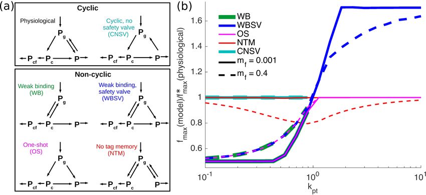
August 14, 2020 8/22Fig 6. Physiological model for glycoprotein quality control outperforms
other models. (a) Schematic of cyclic and non-cyclic models. The physiological model
corresponds to the consensus description of the glycoprotein quality control pathway.
∗
(b) Ratios of folding efficiency fmax comparing performance of all models to the
physiological model. Curve color indicates the model being compared, with solid lines
for mf = 0.001 and dashed lines for mf = 0.4. For all curves, kf = 1.
efficiency for low unbinding rates k-c . This effect is not seen for slowly folding proteins,
which can be released from the chaperones sufficiently rapidly by the standard
deglucosylation pathway (kr ). On the other hand, if the unbinding rate becomes much
higher than the folding rate, then there is a tendency for proteins to detach from the
chaperone before they can fold, manifesting as low values of Pc (Fig. 5b). Thus, very
rapid unbinding reduces the efficiency of the system for both rapidly folding and slowly
folding cases (Fig. 5a).
Figure 5 suggests that different rates of chaperone unbinding (k-c ) become optimal
in different regimes, depending on whether protein production is sufficiently high and
folding is sufficiently slow to overwhelm the available quantity of chaperones.
Chaperones in the ER, such as BiP, are thought to be present in excess
quantities [51–53], to facilitate rapid chaperone binding of nascent proteins. This
suggests that the glycoprotein quality control pathway typically operates in the regime
of relatively low production kpt . 1, so that protein release from chaperones can keep
up with the incoming proteins and the chaperones do not become overwhelmed. At low
protein production, Fig. 5 shows high values of k-c primarily decrease the maximum
folding fraction. Removing the ability of a protein to detach from a chaperone without
glucose trimming should thus improve the performance of the chaperone binding cycle,
and folding proteins should be tightly bound to the chaperone until glucose removal.
This tight binding may have additional functional importance, such as facilitating
recruitment of other enzymes important for folding [30, 54] or as a by-product of the
high specificity of chaperone-glucose interaction [55].
Figures 4 and 5 demonstrate that removing non-specific chaperone binding (k-r ) and
detachment of proteins from the chaperone without glucose trimming (k-c ) improves the
performance of the chaperone binding cycle by increasing the maximum folding fraction
with a limited accumulation of unfolded protein. The consensus physiological model,
with these two processes absent, is thus shown to be more efficient (in the
low-production regime) than the full model illustrated in Fig. 1.
We now explore further glycoprotein quality control pathway model variations,
including those that are not cyclic (Fig. 6a). The non-cyclic models include all possible
variations of a three-state model that lack untagged binding (no k-r ) and are capable of
August 14, 2020 9/22producing a finite steady-state solution. We compare the performance of these models
∗
to the consensus physiological model in terms of the efficiency metric fmax , at varying
levels of protein production (Fig. 6b).
The WB (weak binding) model allows proteins to bind and unbind from the
chaperone, until the glucose tag is removed. The WBSV (weak binding, safety valve)
model introduces an additional “safety-valve” pathway where the glucose tag can be
removed without chaperone binding. The OS (one shot) model treats chaperone binding
and glucose trimming as irreversible, so that each protein only has one chance to
attempt folding. These three models share a common feature – they lack the ability to
restore a glucose tag once it is removed, irreversibly committing deglucosylated proteins
(P ) to degradation. Each of these models performs worse than the physiological system
∗
in the regime of low protein production (kpt < 1), with the folding efficiency fmax
dropping by approximately a factor of 2 (Fig. 6b). In the regime of high production, the
WBSV model is capable of more effectively funneling proteins into a
degradation-committed state, allowing it to significantly outperform the physiological
model (Fig. 6b). However, as discussed previously, cells are believed to typically operate
in a regime of limited protein production levels and excess chaperone capacity, so that
we focus largely on model performance at low kpt .
In the physiological model, a deglucosylated protein (P ) is more likely to have first
passed through chaperone binding than a monoglucosylated protein (Pg ). This feature
allows glucose moieties to serve as a form of molecular memory – the presence of a
glucose tag means the protein is more likely to be newly made; the absence of the tag
means the protein is more likely to have already attempted folding. A contrasting
non-cyclic model is the NTM (no tag memory) model, which allows chaperone binding
and glucose removal to function as independent processes (Fig. 6a). When the fraction
of misfolded proteins (mf ) is low, the NTM model performs equivalently to the
physiological model. However, when a substantial number of proteins entering the
quality control cycle are incapable of being folded (high mf ), the NTM model is at a
disadvantage to the physiological system (Fig. 6b). In the presence of such defective
unfoldable proteins, the cyclic addition and removal of glucose tags allows the
physiological model to have a memory of which proteins already attempted (and failed)
folding and thus should be made vulnerable to degradation. Overall, the physiological
model outperforms all non-cyclic models in the low-production regime.
The cyclic model with no safety valve (CNSV) exhibits the same cycle as the
physiological model: of chaperone binding, deglucosylation upon release, and subsequent
reglucosylation (Fig. 6a). However, it lacks the direct transition from the tagged state
Pg to the vulnerable state P . In the absence of this safety valve pathway, the CNSV
model matches the performance of the physiological model at low production rates
(Fig. 6b). However, for kpt > 1, proteins cannot be released from the chaperones fast
enough to keep up with new protein production, and the CNSV model cannot reach a
steady-state. In this regime, all chaperones would become clogged with protein and the
protein would accumulate indefinitely. A similar behavior is observed for the non-cyclic
WB model, which also lacks the safety-valve (Fig. 6b).
Performance and robustness of the physiological model
We now explore the performance of the physiological model, as well as the optimal
kinetic parameter values under different conditions. Performance is quantified in terms
∗
of the folding efficiency fmax (the maximum folding fraction at a total protein content
Ptot = 1). We treat the total production rate kpt , protein folding rate kf , and misfolding
fraction mf as external input conditions for the system. As always, these rates are
expressed relative to the rate of chaperone removal (kr = 1 for non-dimensionalization),
which is also treated as fixed. The quality control pathway is then allowed to adjust all
August 14, 2020 10/221 10 3 1 10 3 1 10 3
(a) (b) (c)
0.75 0.75 0.75
Optimal ki
Optimal ki
Optimal ki
kc
fmax
fmax
fmax
0.5 1 0.5 1 0.5 1
*
*
*
kg
k -g
0.25 kd 0.25 0.25
0 10 -3 0 10 -3 0 10 -3
10 -1 10 0 10 1 10 -1 10 0 10 1 10 -3 10 -2 10 -1 10 0
kpt kf mf
Fig 7. Optimal performance and corresponding parameters. Maximum
folding fraction fmax at Ptot = 1, (blue curves, left blue vertical axis), and
corresponding optimal rate constants, ki (red curves with markers, right red vertical
axis) as cycle conditions are varied for the physiological model. (a) varies protein
production rate kpt for fixed mf = 10−3 and kf = 1, (b) varies protein folding rate
constant kf for fixed mf = 10−3 and kpt = 0.9, and (c) varies misfolded fraction mf for
fixed kpt = 0.7 and kf = 1.
other kinetic rate constants to optimize the folding efficiency – the resulting optimal
folding fraction and the optimized parameters are plotted in Fig. 7.
When the overall production rate is low, the optimal folding fraction approaches one
(blue curve in Fig. 7a), indicating that nearly all the foldable proteins that enter the
quality control cycle are successfully folded. At higher production (kp & 1), the removal
of proteins from chaperones cannot keep up with the flux of incoming proteins. In this
regime, the available chaperones in the system are overwhelmed and the folding
efficiency drops.
The optimal parameters (red curves in Fig. 7a) describe how the optimized quality
control system adjusts to changing production rates. For all conditions explored,
binding rate constant (kc ) is always maximized, allowing nascent or reglucosylated
proteins to bind to chaperones as quickly as possible. For low kpt , the reglucosylation
rate constant kg is high and the rate constant k-g for glucose removal from free (not
chaperone bound) proteins is low. High kg and low k-g indicate that the cycle is quickly
removing proteins from the vulnerable state P to prevent degradation, which is
expected for low protein production (kpt ) and low misfolded fraction (mf ) as proteins
will then usually be provided multiple rounds of chaperone binding. In this regime, the
optimal degradation rate (kd ) rises gradually with increasing production in order to
maintain a constant amount of unfolded protein Ptot = 1. Eventually (when kpt → 1)
there will not be sufficient chaperones to fold all proteins, and protein degradation must
increase sharply to maintain a fixed level of total unfolded protein.
As the production rate passes kpt ≈ 1, protein reglucusylation (kg ) steeply decreases
and glucose removal (k-g ) increases. This switch indicates the activation of the ‘safety
valve’ pathway which moves excess proteins directly into the degradation-vulnerable
state P to avoid accumulation of unfolded proteins. As protein production continues to
increase, glucose removal via k-g further increases to enhance this safety valve. Overall,
there are two regimes: low protein production, where chaperones are available and
proteins are quickly tagged for chaperone rebinding to prioritize folding; and high
protein production, where chaperones are overwhelmed and rapid deglucosylation and
degradation is prioritized.
Figure 7b shows how performance and optimal parameters change as protein folding
speed kf is varied. As expected, the folding fraction increases with folding speed. The
increased folding speed does not cause significant changes in the optimal parameters,
August 14, 2020 11/221
f(ki optimized at )/fmax
Ptot(ki optimized at )
10 6
*
0.9
All ki xed at
0.8 10 4
0.7
10 2
m f = 0.001
0.6
m f = 0.4
10 0
0.5
(a) (b)
Only kd optimizes
1
f(ki optimized at )/fmax
Ptot(ki optimized at )
10 6
*
0.9
0.8 10 4
0.7
10 2
0.6
10 0
0.5
(c) (d)
10 -1
10 0
10 1
10 -1 10 0 10 1
kpt kpt
Fig 8. Robustness of quality control cycle to changing production rates. (a)
The folding fraction achieved with fixed rate constants is plotted as a fraction of the
maximum achievable folding fraction fmax for Ptot = 1 as the protein production rate
kpt is varied. Fixed rate constants kc , kg , k-g , and kd are those that achieve fmax with
mf = 0.001 at various protein production levels: kpt = 0.1 (red curves and star), kpt = 1
(green), and kpt = 10 (blue). (b) The Ptot corresponding to the folding fractions in (a).
(c) Analogous plot to (a), with rate constants fixed at the optimal values for specific kpt
values, except that the degradation rate constant kd adjusts to maintain Ptot = 1. If kd
adjustment cannot achieve Ptot = 1, then kd adjustment minimizes the difference from
Ptot = 1. (d) The Ptot corresponding to the folding fractions in (c).
with a modest increase in reglucosylation (kg ) and decreases in glucose removal (k-g )
and degradation (kd ) as faster folding frees up chaperones. Figure 7c shows that
increasing the misfolded fraction mf modestly decreases the folding efficiency while
leaving optimal parameters largely unchanged.
Overall, Fig. 7 demonstrates that maintaining maximum folding efficiency requires
large variation in parameters if the protein production level changes, but limited
variation in parameters for changes to protein folding speed and misfolded protein
fraction. We next proceed to explore how well the cycle can perform under changing
production levels if a single fixed parameter set is used across all values of kpt . The goal
is to assess the robustness of this quality control system to changes in protein
production, for the case where other parameters cannot be adjusted sufficiently rapidly
to keep up with such changes.
We consider the robustness of a fixed quality control system as follows. The rate
constants are optimized to give maximal folding efficiency for a given value of input
conditions kpt , kf , mf . For those parameters and input conditions, the system gives the
∗
highest folding fraction fmax that maintains a fixed protein content Ptot = 1. When the
input production rate kpt is varied and all remaining parameters are held fixed, the
folding fraction will decrease below this optimum value (Fig. 8a) and the total protein
content Ptot will also change (Fig. 8b). The values plotted in Fig. 8a,b are given relative
to the folding fraction and protein content at the point where the system was optimized.
If the parameters are optimized at low protein production (kpt = 0.1), the system
August 14, 2020 12/22continues to achieve close to the optimal folding fraction when the protein production is
increased (Fig. 8a, red curves). However, the total accumulated protein increases by
orders of magnitude even for a modest rise in the production rate (Fig. 8b, red curves).
If the parameters are optimized at high protein production (kpt = 10), and the
production rate is lowered significantly, then the folding efficiency is reduced to roughly
half of the optimal amount and the accumulated protein is also decreased (Fig. 8a,b,
blue curves). A system optimized at intermediate production (kpt = 1) exhibits
analogous behaviors (Fig. 8a,b, green curves). If the production rate is lowered, the
folded fraction drops below optimal values. If raised, then a massive increase in
accumulated protein is observed.
These results highlight a general principle: the quality control cycle can be optimized
to operate in one of two regimes: a regime with excess chaperone capacity, and one
where the chaperones are overwhelmed. Optimizing for the former requires shutting off
the safety-valve, and prioritizing reglucosylation over degradation. Optimizing for the
latter requires enhancing degradation and deglucosylation. The transition between the
two regimes occurs when the rate of protein production becomes comparable to the rate
at which chaperone-bound proteins detach from chaperones (i.e.: at kpt = 1). A system
optimized for low production will result in large-scale protein accumulation if the
production rate is increased by even a modest amount. A system optimized for high
production yields suboptimal folding throughput if shifted to the low-production regime.
Without any flexibility to adjust cycle parameters, the glycoprotein quality control
system will perform poorly in one of the two regimes. A natural question is to what
extent adjusting a single kinetic parameter will allow the system to compensate for
changing production rates and to perform well across a broad range of conditions.
Figure 7a shows that the optimal degradation rate (kd ) continuously changes across a
range of low protein production levels (kpt ), suggesting kd as a good candidate for an
adjustable parameter. Thus we choose to treat the degradation rate kd as capable of
adapting to changing production levels, while all other rate constants in the cycle are
held fixed. At each value of the production rate, kd is adjusted to maintain a total
protein content Ptot = 1 whenever possible, with the resulting folding fraction shown in
Fig. 8c. For a system optimized at low protein production, an adjustable degradation
rate allows the optimum folding fraction to be maintained across all production rates.
Even when the fraction of misfolded proteins is increased (dashed curves in Fig. 8c), the
optimum folding fraction can be maintained up to intermediate production levels.
Strikingly, a system optimized at low protein production can also maintain a fixed
total protein Ptot = 1 up to intermediate production levels (kp . 0.7) by adjusting the
degradation rate kd (Fig. 8d). The ability of this system to maintain fixed total protein
content over a broad range of low to intermediate production values is in sharp contrast
to the rapidly increasing protein levels that arise when all parameters are held fixed
(Fig. 8b). At higher production rates, there is no value of the degradation rate that can
maintain the fixed total protein content and we adjust kd as needed to minimize Ptot .
Allowing kd to adjust in a system optimized for intermediate or high protein production
has little impact on both folding fraction and protein accumulation compared to the
fully fixed system (Fig. 8c,d).
This analysis establishes that the quality control pathway can perform well at
typical low production rates, yet be capable of adapting to moderate surges in protein
production. Such robust behavior requires only for the protein degradation rate to be
rapidly adjustable to changing conditions. Other parameters in the quality control cycle
can be held constant while allowing near-optimal system performance over an order of
magnitude range in protein production. Interestingly, there is evidence that cellular
quality control systems do in fact control protein degradation throughput in response to
perturbations in protein homeostasis. Specifically, cells maintain a reservoir of ERAD
August 14, 2020 13/22enzymes in ER-associated vesicles that can fuse with the ER lumen in response to an
accumulation of unfolded proteins, rapidly upregulating protein degradation [56–58].
Discussion
We have investigated the impact of pathway architecture and kinetic parameters on the
performance of the glycoprotein quality control cycle in the endoplasmic reticulum.
Two metrics are used to evaluate steady-state performance. The fraction of foldable
proteins that are successfully folded measures the accuracy of the system. The total
quantity of unfolded proteins measures processing speed, with lower protein levels
corresponding to more rapid processing.
Broadly, we find that a cyclic quality control process, with protein substrates driven
in a preferred direction through three quality control states, leads to improved
performance. Energy is required for cyclic driving, and increased driving energy per
cycle allows higher protein folding fractions (Fig. 3). A higher folding fraction is
achieved by eliminating reverse transitions that are absent from the consensus
physiological model of the glycoprotein quality control pathway (Figs. 4 and 5). This
matches the directed, cyclic behavior commonly described as occurring for physiological
glycoprotein quality control.
The energy-consuming nature of the quality control cycle improves its decision
making during the protein folding process, echoing other examples of biomolecular
processes cyclically driven out of equilibrium to improve their performance. DNA
copying is famously driven out of equilibrium in a ‘kinetic proofreading’ process that
increases its accuracy [3, 59]. Similar cyclic nonequilibrium processes increase the
accuracy of T-cell signaling [4] and sensing of external concentrations [60].
By exhaustively considering all remaining cyclic and non-cyclic variations of the
glycoprotein quality control pathway, we show that the consensus physiological model
outperforms all other viable models (Fig. 6). Models lacking a ‘safety valve’, or a path
for protein degradation without chaperone binding, will dangerously accumulate
unfolded proteins at high protein production levels. This safety valve requirement aligns
with the only two-way transition in the consensus physiological model, which allows
glucose tags to be removed from proteins that are not bound the chaperone, facilitating
their degradation.
We find that the optimal tuning of the consensus physiological model varies
substantially with protein production level (Fig. 7a). If the cell must choose a particular
set of rate constants, it will either sacrifice folded protein throughput at low protein
production levels, or induce massive unfolded protein accumulation at higher production
levels (Fig. 8a,b). A particularly robust system design requires optimizing parameters
for low protein production and allowing a single rate constant (the degradation rate) to
adapt to changing production levels. Such a system can successfully maintain both
maximum folding efficiency and low unfolded protein accumulation across a range of
low-to-intermediate production rates (Fig. 8c,d).
In vivo glycoprotein folding in the ER is thought to operate in a low protein
production regime, matching the robust system design. Namely, there is excess protein
folding capacity in the ER under basal conditions [51], with abundant chaperones that
exceed the requirements of the protein folding load [52, 53]. Under conditions of high
protein folding load, chaperones are overwhelmed [61, 62], and the unfolded protein
response is triggered, driving down the effective protein folding load by increasing
chaperone quantity [51] and reducing protein translation [63].
The adjustable degradation rate, which alone can maintain both high folding
throughput and low unfolded protein accumulation, corresponds to the dynamic
behavior observed for some ERAD enzymes that remove proteins from the ER for
August 14, 2020 14/22degradation. Certain mannosidases, important for ERAD targeting, are largely
sequestered to quality control vesicles in the absence of ER stress [56–58]. When the ER
becomes stressed (i.e. unfolded proteins accumulate), these mannosidases converge on
the ER, rapidly increasing degradation targeting [56–58]. Comparison of timescales for
mannosidase convergence to the ER following proteasome inhibition (approximately a
couple hours [51]) and the gene expression response to accumulation of unfolded
proteins (approximately 5 to 10 hours [57]) indeed suggests that ERAD-mediated
degradation may be enhanced relatively quickly.
In contrast to the large variations in optimal rate constants with protein production
level, changes in protein folding speed require relatively little variation to the optimal
rate constants (Fig. 7b). The glycoprotein quality control pathway must simultaneously
process a variety of proteins, which can have folding times ranging from a few minutes
to several hours [31]. The ability of a single pathway to near-optimally process this
variety of folding speeds appears to be a strength of its design. The efficiency of protein
throughput can approach 100% and range down to 25% or lower for slow-folding
proteins or proteins with mutations [31]. Fig. 7b suggests that these low efficiencies
(ranging down to 25% or lower) are not the result of a poorly-tuned quality control
process, but instead that the low efficiencies are an unavoidable consequence of slow
folding.
The optimal rate constants also change little with the fraction of produced proteins
which are inherently misfolded or unfoldable (Fig. 7c). This suggests the design of the
quality control pathway is robust to the onset of systematic misfolding, which may arise
from translation errors, environmental stress, or mutations [46], so long as the total
protein production levels remain relatively unchanged.
Effective quality control of glycoprotein folding in the endoplasmic reticulum ensures
an adequate supply of functional natively-folded proteins and limits the accumulation of
misfolded proteins. The failure to provide sufficient natively-folded proteins [31] and the
formation of misfolded protein aggregates [9] can both contribute to the onset of disease.
Our modeling quantitatively demonstrates how the performance of this pathway under
a broad range of conditions is modulated by key kinetic parameters that serve as
potential targets for pharmacological or genetic perturbations. This quantitative
framework serves as a basic foundation for understanding the glycoprotein quality
control pathway, which can be further expanded in future work to account for more
complex aspects, such as sequential glycan sugar moiety removal [40, 57] and the spatial
organization of quality control activities [56].
Methods
Non-dimensionalization
We non-dimensionalize all times by the timescale of protein removal from the chaperone
via glucose trimming, kr−1 , and all concentrations by total chaperone concentration,
Ctot . For conciseness of notation, all kinetic parameters in the text refer to
non-dimensionalized values. The dimensionless dynamic equations for foldable proteins
August 14, 2020 15/22are then:
dPg
= kg P + k-c Pc − (kc CA + k-g )Pg + kp (4a)
dt
dPc
= (kc Pg + k-r P )CA − (1 + k-c + kf )Pc (4b)
dt
dP
= Pc + k-g Pg − (kg + k-r CA − kd )P (4c)
dt
dPcf
= kf Pc − (1 + k-c )Pcf , (4d)
dt
dPcb
= k-r CA Pb − kr Pcb . (4e)
dt
The dynamics of misfolded proteins are described by
dPg∗
= kg P ∗ + k-c Pc∗ − (kc CA + k-g )Pg∗ + kp∗ (5a)
dt
dPc∗
= (kc Pg∗ + k-r P ∗ )CA − (1 + k-c )Pc∗ (5b)
dt
dP ∗
= Pc∗ + k-g Pg∗ − (kg + k-r CA − kd )P ∗ . (5c)
dt
Note that most rate constants are the same for both foldable and misfolded proteins,
except kp changes to kp∗ to allow different production rates of foldable and misfolded
proteins, kf∗ = 0 (misfolded proteins cannot fold), and Pb∗ = 0 (as only a single
comprehensive population of background proteins is considered). The available amount
of chaperone is CA = 1 − Pc − Pcf − Pc∗ − Pcb , where Ctot = 1 is the dimensionless total
chaperone concentration.
Steady-state solution of chaperone cycle dynamics
Equations 4 and 5 describe the dynamics of the chaperone folding cycle. In steady state
each of the time derivatives must equal zero. By summing together Eqs. 4a–d, we get
the steady-state condition for the total flux of foldable proteins through the cycle:
kp = kf Pc + kd P . (6)
Rearranged, this gives P in terms of parameters and Pc ,
kp kf
P = − Pc . (7)
kd kd
Applying dPcf /dt = 0 gives
kf
Pcf = Pc , (8)
kr + k-c
and dPcb /dt = 0 gives
Pcb = k-r Pb CA , (9)
where the available chaperone is
CA ≡ 1 − Pc − Pcf − Pc∗ − Pcb (10a)
kf
=1− 1+ Pc − Pc∗ − k-r Pb CA . (10b)
kr + k-c
August 14, 2020 16/22Substituting Eqs. 7, 8, and 9 into Eqs. 4a,b gives
dPc k-r kp k-r kf
= C A k c Pg + − Pc − (kf + 1 + k-c )Pc (11a)
dt kd kd
dPg kg kp kg kf
= kp + k-c Pc + − Pc − k-g Pg − CA kc Pg . (11b)
dt kd kd
Similarly for misfolded proteins, which have kf∗ = 0, the steady state condition for
protein fluxes entering and exiting the cycle is
kp∗
P∗ = . (12)
kd
Substituting Eq. 12 into Eqs. 5a,b gives
dPc∗ k-r kp∗
∗
= CA kc Pg + − (1 + k-c )Pc∗ (13a)
dt kd
dPg∗ kg kp∗
= kp∗ + k-c Pc∗ + − k-g Pg∗ − CA kc Pg∗ . (13b)
dt kd
Equation 11 can be rewritten as MP~ = ~b:
CA kc CA m1 + n1 Pg CA b1
~
MP = = = ~b , (14)
−CA kc − k-g n2 Pc b2
with m1 = −k-r kf /kd , n1 = −(kf + 1 + k-c ), n2 = k-c − kg kf /kd , b1 = −k-r kp /kd , and
b2 = −(kp + kg kp /kd ). The determinant
2 2
|M| = kc m1 CA + (k-g m1 + kc n1 + kc n2 )CA + k-g n1 = r2 CA + r1 CA + r0 . Rearranging
gives
Pg 1 p1 CA + p0
= 2 +r C +r 2 , (15)
Pc r2 CA 1 A 0 q2 CA + q1 CA
with p1 = b1 n2 − m1 b2 , p0 = −b2 n1 , q2 = kc b1 , q1 = k-g b1 + kc b2 .
Similarly, Eq. 13 can be rewritten as M∗ P~ ∗ = ~b∗ :
n∗1 Pg∗ CA b∗1
CA kc
M∗ P~∗ = = = ~b , (16)
−CA kc − k-g k-c Pc∗ b∗2
with n∗1 = −(1 + k-c ), b∗1 = −k-r kp∗ /kd , and b∗2 = −kp∗ − kg kp∗ /kd . The determinant
|M∗ | = CA (kc k-c + n∗1 kc ) + n∗1 k-g = CA r1∗ + r0∗ . Rearranging gives
∗ ∗
p1 CA + p∗0
Pg 1
= , (17)
Pc∗ CA r1∗ + r0∗ q2∗ CA2
+ q1∗ CA
with p∗1 = k-c b∗1 , p∗0 = −b∗2 n∗1 , q2∗ = kc b∗1 , and q1∗ = k-g b∗1 + kc b∗2 .
We now insert Pc from Eq. 15 and Pc∗ from Eq. 17 into Eq. 10b,
2
kf q2 CA + q1 CA
CA = 1 − 1 + 2
1 + k-c r2 CA + r1 CA + r0
q2∗ CA2
+ q1∗ CA k-r
− − Pb CA . (18)
r1 CA + r0∗
∗ kr
Rearranging,
CA (1 + k-r Pb )[r2 r1∗ CA
3
+ (r2 r0∗ + r1 r1∗ )CA
2
+(r1 r0∗ + r0 r1∗ )CA + r0 r0∗ ]
−[r2 r1∗ CA
3
+ (r2 r0∗ + r1 r1∗ )CA
2
+ (r1 r0∗ + r0 r1∗ )CA + r0 r0∗ ]
2
+[1 + kf /(k-c + 1)](q2 CA + q1 CA )(CA r1∗ + r0∗ )
+(q2∗ CA
2
+ q1∗ CA )(r2 CA
2
+ r1 CA + r0 ) = 0 . (19)
August 14, 2020 17/22This forms a quartic equation for CA , which can be solved with standard root-finding
algorithms. Once CA is obtained, Eqs. 15 and 17 give steady state Pc , Pg , Pc∗ , and Pg∗ ,
from which Eq. 7 gives steady state P . Eq. 12 gives steady state P ∗ once kp∗ and kd are
selected, without needing other information.
Optimization of cycle efficiency
For the results in Fig. 2, the maximum folding fraction independent of total unfolded
protein was first found by allowing ki = kc , k-c , kg , k-g , k-r , and kd to vary to maximize
the folding fraction using the Matlab routine fmincon, with ki ∈ [10−3 , 103 ]. The
minimum total unfolded protein is found using the Matlab routine fmincon for each
fixed folding fraction (at a value less than or equal to the maximum folding fraction),
constrained with the nonlinear constraints option, and with ki ∈ [10−3 , 103 ].
For the results in Fig. 3, ki = kc , k-c , k-r , kg , k-g , and kd are allowed to vary to
maximize the folding fraction (Eq. 2), while fixing the energy (Eq. 3) at a specific value,
and fixing the total unfolded protein Ptot = 1. The folding fraction maximization was
performed using the Matlab routine fmincon with energy and total unfolded protein
fixed using the nonlinear constraints option. The ki were free within the range
ki ∈ [10−3 , 103 ].
The results in Fig. 4 are found similarly to those of Fig. 2, with the fixed folding
fraction varied using the bisection method until a Ptot ∈ (0.99, 1.01) is found. Results in
Figs. 5 and 7 are found with the same method as Fig. 4 with the appropriate ki set to
zero and the appropriate ki allowed to vary within ki ∈ [10−3 , 103 ]. Almost all results in
Fig. 6 are also found with the method of Figs. 5 and 7. The exception in Fig. 6 is the no
tag memory (NTM) model, which lacks the transition represented with rate constant kr ,
and instead sets k-c = 1.
∗
The fmax and optimizing ki∗ at particular kpt in Fig. 8 are found with the same
∗
method as Figs. 4, 5, 6, and 7. The optimal parameters that achieve fmax are then used
as the fixed parameters in Eq. 19 to determine the folding fraction and total unfolded
protein in Fig. 8a,b as the protein production is varied. The folding fraction and total
unfolded protein in Fig. 8c,d with only kd free is found by using the bisection method to
vary kd to attempt to find a kd value with Ptot = 1. If Ptot = 1 cannot be achieved with
kd ∈ [10−3 , 103 ] then kd = 103 is chosen to minimize Ptot .
Acknowledgments
This work was supported in part by funding from the Hellman Fellows Fund, the Alfred
P. Sloan Foundation, and a Cottrell Scholars Award from the Research Corporation for
Science Advancement.
References
1. Murrow L, Debnath J. Autophagy as a stress-response and quality-control
mechanism: implications for cell injury and human disease. Annual Review of
Pathology: Mechanisms of Disease. 2013;8:105–137.
2. Pohl C, Dikic I. Cellular quality control by the ubiquitin-proteasome system and
autophagy. Science. 2019;366(6467):818–822.
3. Hopfield JJ. Kinetic proofreading: a new mechanism for reducing errors in
biosynthetic processes requiring high specificity. Proceedings of the National
Academy of Sciences. 1974;71(10):4135–4139.
August 14, 2020 18/22You can also read


