Automated segmentation of microtomography imaging of Egyptian mummies
←
→
Page content transcription
If your browser does not render page correctly, please read the page content below
Automated segmentation of microtomography imaging of
                                                    Egyptian mummies
                                                    Marc Tanti1¤ , Camille Berruyer2 , Paul Tafforeau2 , Adrian Muscat1 , Reuben Farrugia1 ,
                                                    Kenneth Scerri3 , Gianluca Valentino1 , V. Armando Solé2 , Johann A. Briffa1*

                                                    1 Dept. of Comm. & Computer Engineering, University of Malta, Msida MSD 2080,
                                                    Malta
arXiv:2105.06738v1 [cs.CV] 14 May 2021

                                                    2 European Synchrotron Radiation Facility, 71 Avenue des Martyrs, CS-40220, 38043
                                                    Grenoble cedex 09, France
                                                    3 Dept. of Systems & Control Engineering, University of Malta, Msida MSD 2080, Malta

                                                    ¤Current Address: Institute of Linguistics & Language Technology, University of Malta,
                                                    Msida MSD 2080, Malta
                                                    * johann.briffa@um.edu.mt

                                                    Abstract
                                                    Propagation Phase Contrast Synchrotron Microtomography (PPC-SRµCT) is the gold
                                                    standard for non-invasive and non-destructive access to internal structures of
                                                    archaeological remains. In this analysis, the virtual specimen needs to be segmented to
                                                    separate different parts or materials, a process that normally requires considerable
                                                    human effort. In the Automated SEgmentation of Microtomography Imaging (ASEMI)
                                                    project, we developed a tool to automatically segment these volumetric images, using
                                                    manually segmented samples to tune and train a machine learning model. For a set of
                                                    four specimens of ancient Egyptian animal mummies we achieve an overall accuracy of
                                                    94–98% when compared with manually segmented slices, approaching the results of
                                                    off-the-shelf commercial software using deep learning (97–99%) at much lower
                                                    complexity. A qualitative analysis of the segmented output shows that our results are
                                                    close in term of usability to those from deep learning, justifying the use of these
                                                    techniques.

                                                    Introduction
                                                    For at least a decade, archaeologists have been interested in applying new technologies
                                                    to their research to better understand our past. State-of-the-art Propagation Phase
                                                    Contrast Synchrotron Microtomography (PPC-SRμCT) is becoming a golden standard
                                                    for a non-invasive and non-destructive access to internal structures of archaeological
                                                    remains. This technique has been recently applied to archaeozoological studies of
                                                    mummified animal remains from the Ptolemaic and Roman periods of ancient Egypt
                                                    (around 3rd century BC to 4th century AD). Researchers performed virtual autopsies
                                                    and virtual unwrapping, uncovering information about animal life and death in past
                                                    civilisations, as well as revealing the processes used to make these mummies [1, 2].
                                                    However, this can be a long process. After microtomographic data processing and
                                                    reconstruction, the virtual specimen has to be segmented to separate the different parts
                                                    or different materials of the sample. For biological samples, such as animal mummies,
                                                    segmentation is usually done semi-manually, and can require weeks of human effort,

                                     May 17, 2021                                                                                      1/28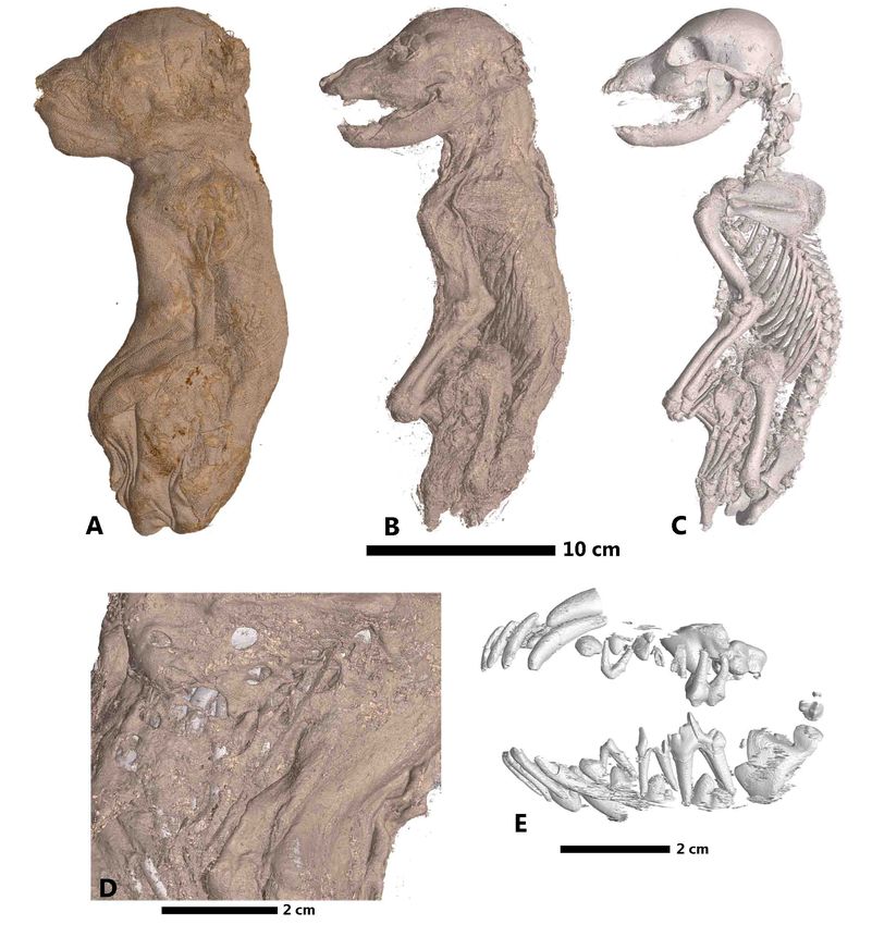
even for small volumes. Effective automatic segmentation based on Artificial
               Intelligence (AI) could drastically reduce this effort, with the expected computation
               time reduced to a matter of hours, depending on the size and complexity of the
               volumetric image. This is particularly relevant as the number and sizes of volumes
               increases. For example, the European Synchrotron Radiation Facility (ESRF) is
               currently generating huge amounts of data of human organs (up to 2 TiB for a single
               scan); only AI approaches can handle segmentation at this scale.
                   Automatic segmentation is well-developed in medical imaging, such as the CHAOS
               Challenge [3] task for segmenting the liver from a human CT scan, where many of the
               top-ranking methods are variations on the deep learning neural network U-Net [4]. By
               contrast, in archaeology, the problem is less well-studied, and the techniques available
               are less sophisticated. For example, Hati et al. [5] segmented an entire human mummy
               into jewels, body, bandages, and the wooden support frame, using a combination of
               voxel intensity and the manual selection of geodesic shapes. Low resolution volumetric
               scans of mummies were considered in [6, 7], with segmentation performed one slice at a
               time using classical machine learning techniques. In both works, ridged artifacts and
               loss of detail were evident in the results obtained.
                   The automatic segmentation in commercially available software for volumetric
               editing, such as Dragonfly [8], requires a human expert to manually segment a small
               subset of slices from the tomography image with all the parts that need to be identified.
               A machine learning model is then trained from the manually segmented examples and
               used to segment the rest of the volume. In the Automated SEgmentation of
               Microtomography Imaging (ASEMI) project, we developed a fully automatic segmenter
               using the same methodology, based on classical machine learning. Our approach has a
               number of advantages over commercial solutions. Specifically, our segmenter is not
               limited by the computer’s main memory, allowing it to segment arbitrarily large
               volumes (e.g. the largest scan presented here requires 133 GiB for the volume itself, and
               a further 66 GiB for the labels, while the feature vectors would require several TiB). Its
               parameters are automatically optimised for the given volume, minimising user input. It
               also works directly with three dimensional features, rather than reducing the problem to
               an independent segmentation of two-dimensional slices, without increasing
               computational complexity from quadratic to cubic. This allows our system to scale well,
               particularly for larger volumes. Finally, our system can use interpretable machine
               learning models, making it possible to inspect the reasons behind segmentation errors.
                   Our output segmentations have an overall accuracy of 94–98% when compared with
               manually segmented slices. This approaches the results of off-the-shelf commercial
               software using deep learning (97–99%) at much lower complexity. A qualitative analysis
               of the outputs shows that our results are close in term of usability to those from deep
               learning. Some postprocessing is necessary to clean up segmentation boundaries, for
               both our system and the deep learning approach.
                   All software and datasets used to generate the results in this work are available for
               free download. The input and output datasets are available under a Creative Commons
               Attribution-NonCommercial-ShareAlike 4.0 International License at the ESRF heritage
               database for palaeontology, evolutionary biology and archaeology [9]. The source code
               has been released under the GNU General Public Licence (GPL) version 3 (or later)
               and can be found, together with its documentation, on GitHub [10]. (Both repositories
               will be opened to the public once the manuscript is accepted for publication.)

May 17, 2021                                                                                       2/28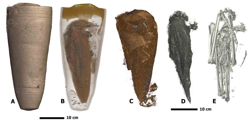
Fig 1. Voxels at different scales. An illustration of a voxel at scale 0 (blue) and its
               corresponding voxel at scale 1 (red). A voxel at scale 1 (red) corresponds to every voxel
               in a 2 × 2 × 2 region at scale 0 (light red).

               Algorithm design
               Overview
               The ASEMI segmenter is an algorithm that determines, for every voxel in a volumetric
               image, a label that corresponds to the material or part that the voxel belongs to. For
               any given volumetric image there may be a number of labels N ≥ 2, where one of the
               labels represents those parts or materials that are not further distinguished (this label
               can be interpreted as ‘background’ or ‘anything else’). The algorithm works by first
               obtaining a descriptive feature vector for every voxel, and then using a classifier to
               determine a label based on the feature vector.

               The voxel neighbourhood
               The feature vector for a given voxel depends on the voxel itself and also on the voxel’s
               context, which is necessary to determine the texture that a voxel forms part of.
               Formally, the feature vector is a function of the voxel neighbourhood at a given scale,
               which are defined as follows. The neighbourhood of radius r is the cube of voxels of side
               2r + 1 centered around the voxel of interest. The scale s is the number of times the
               entire volume is resized by half, so that a neighbourhood can be from the original
               volume (s = 0) or from a smaller version of the volume at the corresponding location of
               the central voxel. These relationships are illustrated in Fig 1. The scaled volumes are
               obtained by first applying a 3D Gaussian blur to the entire volume and then decimating
               this by a factor of 2s in each dimension. This creates versions of the volume with less
               detail, allowing the algorithm to operate on larger-scale textures.

               Feature vectors
               For any given voxel neighbourhood radius and scale, a number of different features may
               be obtained. We usually use a concatenation of several feature vectors, each obtained at
               a different neighbourhood radius and scale, as an input to the classifier.

May 17, 2021                                                                                       3/28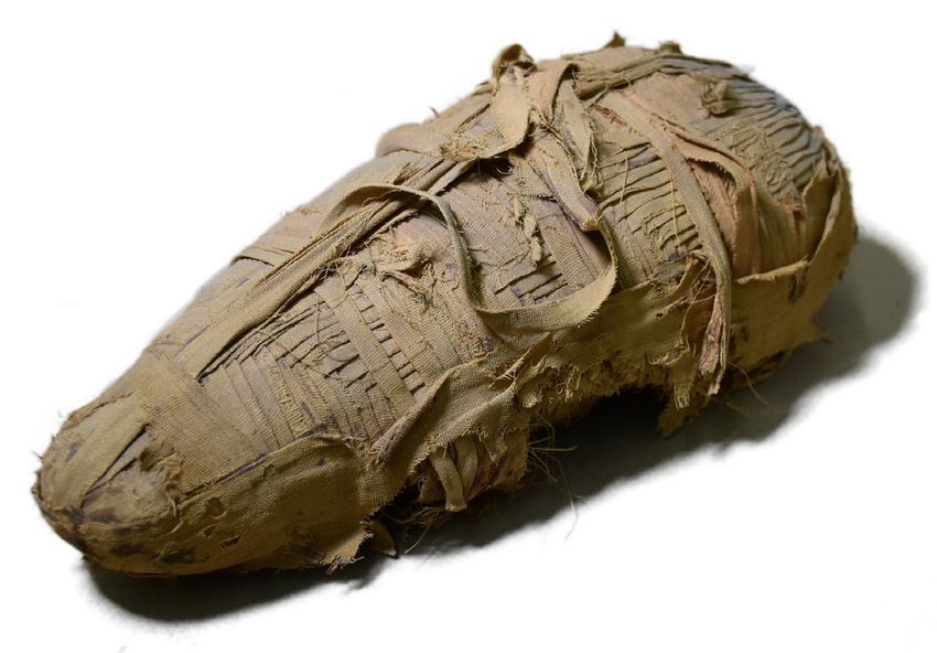
Fig 2. Three orthogonal planes within a voxel neighbourhood. An illustration
               of the three orthogonal planes in the neighbourhood of radius r = 2 for the red voxel in
               the center. The xy, yz, and xz planes are shown in magenta, cyan, and yellow
               respectively.

                   The simplest feature is the intensity value of the voxel being classified, which
               corresponds to the density of the material in that location. Clearly, this feature is
               independent of the neighbourhood radius, and does not carry any information about the
               material texture. While it is possible to consider the intensity at different scale, we
               usually use this feature only at scale zero. Therefore, no parameters are necessary to
               uniquely define this feature.
                   Next up in complexity is the histogram of intensities within the given neighbourhood.
               This feature vector consists of an array of k frequencies, one for each linearly-spaced bin
               of voxel intensities. This contains information about the distribution of material density
               in the given neighbourhood. Computation of this feature vector is defined by three
               parameters: the neighbourhood radius r, scale s, and number of bins k.
                   The distribution of material density is one aspect of the texture that a voxel forms
               part of. Another aspect is the structure of the texture. This is captured well by the
               Local Binary Pattern (LBP) [11], which operates on a plane, and is insensitive to
               density variation but sensitive to the relative location of voxel values. In order to
               capture information in three dimensions, we combine the features from three orthogonal
               planes centered on the voxel under inspection [12, 13], as illustrated in Fig 2 for a
               neighbourhood of radius r = 2. First, an LBP code is obtained for every voxel, based on
               its immediate 3 × 3 neighbourhood in the plane considered (i.e. the 8 neighbours at
               radius 1). Uniform and rotation invariant LBP codes [14] are used, as preliminary
               experiments showed that these improve performance while reducing the feature vector
               size. Next, we obtain a histogram of the codes corresponding to voxels in a 2D
               neighbourhood of radius r in the plane considered, and use this as our feature vector.
               Computation of this feature vector is defined by three parameters: the scale s and
               histogram neighbourhood radius r. The number of histogram bins is fixed to 10, as that
               is the number of different codes possible.
                   Other features exist for encoding textural information, such as SIFT [15] and
               SURF [16], which have found extensive use in computer vision. In preliminary
               experiments we found that these features were computationally much more expensive

May 17, 2021                                                                                        4/28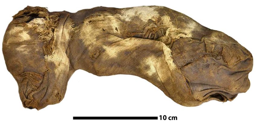
and did not improve performance. Therefore, we did not consider them further for this
               application.
                   The final feature vector chosen is the concatenation of: a) the value of the voxel
               being classified, b) a short range histogram of voxel values at scale zero, c) a long range
               histogram of voxel values (at a scale to be determined), and d) a three orthogonal
               planes LBP (at a scale to be determined). Preliminary experiments showed that the
               combination of histogram and LBP features was better than either one alone. We also
               experimented with two-dimensional histogram across the three orthogonal planes, as
               well as the mean value of the voxel neighbourhood, but the performance increase was
               minimal and did not justify the added complexity. Using both short and long range
               features (both histogram and LBP) resulted in a small performance increase over using
               only long range features. Rather than use long and short range features for both
               histogram and LBP, we opted to limit this to the histogram features which are faster to
               compute.

               Classifier
               The extracted features are used as input to a classifier, which is trained to create a
               mapping between the feature vectors and the corresponding label. Two classifiers are
               used in this work: the random forest classifier [17], as implemented in scikit-learn [18],
               and the feedforward neural network [19] as implemented in Tensorflow [20]. The
               random forest classifier has the advantage of being an interpretable model while the
               neural network generalises well and has a faster GPU-based implementation. We also
               experimented with support vector machines [21], but these were not performing as well
               as the other methods so we did not consider them further.
                   The random forest classifier was trained with a node splitting criterion based on the
               Gini impurity, no limit on the number of leaf nodes, a maximum tree depth of 16, and
               the number of features per tree equal to the square root of the total number of features.
               The only remaining hyperparameter, the number of trees, was left as a free variable to
               be determined in the hyperparameter optimisation process, within the range specified in
               Table 1.
                   Similarly, the neural network structure included two hidden layers with a leaky
               ReLU activation function, and was trained with the Adam optimiser, early stopping
               criterion, dropout, and weight initialisation using normal random numbers with zero
               mean and bias initialisation of zero. The remaining hyperparameters, left as free
               variables to be determined in the hyperparameter optimisation process, are listed in
               Table 1, together with the range explored.
                   The optimisation process consists of a two-stage random search in the combined
               search space of the feature selection variables and model hyperparameters. The first
               stage randomly samples the entire search space; this explores the search space more
               efficiently than a grid search as it samples the space uniformly across all variables,
               rather than prioritising specific variables based on the pre-defined search order. The
               second stage is a local search, starting with the best result from the first stage. The
               algorithm randomly changes a single variable, in an iterative process that is similar to a
               stochastic hill climbing optimiser. Details are outlined in Algorithm 1.

               Implementation Efficiency and Scalability
               Overview
               For the application considered, with microtomography images of 109 to 1010 voxels, the
               scalability of the algorithms is a critical concern. There are two aspects to this: memory

May 17, 2021                                                                                         5/28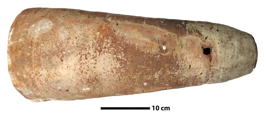
Algorithm 1: Two-stage search algorithm.
                Input: A training set and a validation set.
                Data: A number of global iterations Ig = 1000, a number of local iterations
                       Il = 10000, a number of training set voxel samples St = 16000, a number
                       of validation set voxel samples Sv = 16000, a number of seconds as a
                       timeout limit t = 5.
                Output: An optimised set of variables
                sampledTrainSet ← a sample of St items from each label in the training set
                sampledValSet ← a sample of Sv items from each label in the validation set
                knownVarSets ← ∅
                bestVarSet ← null
                bestAccuracy ← 0
                begin global phase
                   for Ig times do
                      repeat
                           varSet ← a random set of variables
                           if more than t seconds have passed then exit global phase
                      until varSet ∈ / knownVarSets
                      add varSet to knownVarSet
                      segmenterModel ← new segmenter model using varSet
                      train segmenterModel using sampledTrainSet
                      modelAccuracy ← evaluate segmenterModel accuracy using
                        sampledValSet
                      if modelAccuracy > bestAccuracy then
                           bestVarSet ← varSet
                           bestAccuracy ← modelAccuracy
                      end
                   end
                end
                begin local phase
                   for Il times do
                      repeat
                           varSet ← bestVarSet
                           replace a single variable in varSet with a random value
                           if more than t seconds have passed then exit local phase
                      until varSet ∈ / knownVarSet
                      add varSet to knownVarSet
                      segmenterModel ← new segmenter model using varSet
                      train segmenterModel using sampledTrainSet
                      modelAccuracy ← evaluate segmenterModel accuracy using
                        sampledValSet
                      if modelAccuracy > bestAccuracy then
                           bestVarSet ← varSet
                           bestAccuracy ← modelAccuracy
                      end
                   end
                end
                Result: bestVarSet

May 17, 2021                                                                                6/28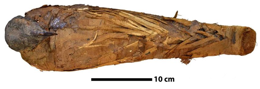
Table 1. Search space for free variables in feature selection and model
               hyperparameters.
               a: Feature selection.

                                       Feature        Variable    Search Space
                                       Histogram 1    Radius            1-8
                                                      Bins         {8, 16, 32}
                                       Histogram 2    Scale             0-2
                                                      Radius           1-32
                                                      Bins         {8, 16, 32}
                                       LBP            Scale             0-2
                                                      Radius           1-32
               b: Model hyperparameters.

                              Classifier       Hyperparameter             Search Space
                              Random forest    Number of trees             {16, 32, 64}
                              Neural network   Layer 1 size             {32, 64, 128, 256}
                                               Layer 2 size             {32, 64, 128, 256}
                                               Dropout rate                   0.0-0.5
                                               Initialisation stddev.       0.0001-1.0
                                               Minibatch size           {4, 8, 16, 32, 64}

               requirement and computational complexity. At this scale, the images are at the limit of
               what will fit in current high-RAM machines, while the set of feature vectors for the
               entire volume will easily exceed available memory. Next-generation scans, such as those
               recently started at the ESRF, generate images that are already larger than available
               memory. It is therefore necessary for the algorithm implementation to divide the
               volume into subvolumes and operate on these separately. In a naive implementation, the
               computational complexity scales linearly with the number of voxels, as the extraction of
               the feature vector can be seen as independent for each voxel. However, neighbouring
               voxels have overlapping neighbourhoods, so that some computations can be shared
               between them. An optimised implementation can leverage this to reduce the overall
               complexity.

               Optimised histogram computation
               The main contributor to the computational complexity of feature extracation is the
               computation of histograms of voxel neighbourhoods, used for both the histogram feature
               vector and the LBP feature vector. When the histogram for each neighbourhood is
               independently computed, the complexity is cubic with respect to the neighbourhood
               radius r. If we incrementally compute histograms for the neighbourhoods of adjacent
               voxels, however, we can reduce the overall complexity to quasi-quadratic.
                   Consider the neighbourhood of radius r of a voxel vx,y,z at index x, y, z in the
               volume. Computing the histogram for this single neighbourhood requires consideration
               of (2r + 1)3 voxel intensities, for a complexity O(r3 ). Now consider the neighbourhood
               of adjacent voxel vx,y,z+1 . This overlaps with the neighbourhood of vx,y,z , except for
               the planes z − r and z + r + 1, as illustrated in Fig 3. Therefore, we can compute the
               neighbourhood histogram for vx,y,z+1 as an incremental change on that of vx,y,z .
               Starting with the histogram for vx,y,z , we subtract the frequencies for the plane z − r
               and add the frequencies for the plane z + r + 1. Each of these two operations requires

May 17, 2021                                                                                      7/28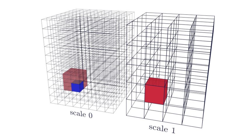
Fig 3. Neighbourhood overlap for adjacent voxels. An illustration of the
               overlap between the neighbourhoods of radius r = 2 for the blue voxel vx,y,z (shown in
               cyan), and the adjacent red voxel vx,y,z+1 (shown in magenta). The plane z − r exists
               only in the first neighbourhood, while the plane z + r + 1 exists only in the second
               neighbourhood.

               consideration of (2r + 1)2 voxel intensities, for an overall complexity O(r2 ) for this
               incremental histogram computation.
                   For any given subvolume, the first neighbourhood histogram needs to be computed
               independently, while all other histograms can be determined incrementally. Assuming
               the subvolume size is much larger than r, the effect on complexity of the first histogram
               becomes insignificant, for an overall complexity approaching O(r2 ).
                   A considerable improvement in efficiency is also obtained by computing histograms
               on a GPU, using NVIDIA’s CUDA framework [22]. For incremental histogram
               computation it is advantageous to consider operations on independent slices. We can
               compute the histograms for each voxel neighbourhood in parallel, because they are
               independent. This allow us to take advantage of the massively parallel GPU
               architecture. Furthermore, observe that even in this case, the neighbourhoods for
               adjacent voxels overlap significantly. We take advantage of this overlap by loading the
               neighbourhood into on-chip ‘shared’ memory, which is accessible at cache-level speeds
               by the computational units of the multiprocessor. This significantly reduces the number
               of memory reads required, for a significant speedup in this I/O-bound problem.
                   We also take advantage of a number of GPU architecture features to ensure an
               efficient implementation. These include the parallel reading of tile neighbourhood data
               into shared memory, organised so that access by warp threads is on different memory
               banks. Incrementally computed histograms are also kept in shared memory, writing only
               the final 3D histogram results to main memory.
                   Note that these improvements are also of benefit when computing LBP features.
               Specifically, for each of the three orthogonal planes, once the LBP codes corresponding
               to each voxel are computed, a histogram of these codes is obtained for the 2D voxel
               neighbourhood of radius r. The computation of the LBP codes takes constant time, as
               for each voxel it requires a comparison with the eight immediate neighbours.
               Computing the histogram of the codes requires consideration of (2r + 1)2 voxel
               intensities, for a complexity O(r2 ). The histogram computation therefore dominates the

May 17, 2021                                                                                       8/28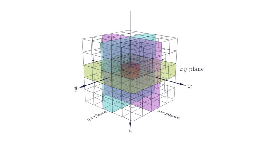
Table 2. Validating speedups on a small volume. Volume size 180 × 150 × 200;
               CPU: Intel Core i7-8700K at 3.7 GHz; GPU: NVIDIA GeForce GTX 1080 Ti.
                                                               CPU (s) GPU (s)
                             Histogram (r = 32, s = 0, k = 32)  17.8     1.1
                             LBP (3-plane, r = 32, s = 0)       24.4     1.3

               complexity of the LBP feature extraction.
                  Comparative timings were obtained during development to validate these
               optimisation steps. Table 2 gives the time taken for the feature extraction process on a
               small 180 × 150 × 200 volume using an Intel Core i7-8700K CPU at 3.7 GHz and an
               NVIDIA GeForce GTX 1080 Ti. In all cases, histograms are computed using the
               incremental algorithm.

               Complexity analysis and comparison with U-Net
               The overall complexity of the ASEMI segmenter can be determined by considering both
               the feature extraction and the classifier. The complexity for computing the features
               depends directly on the neighbourhood radius r, as already shown. When incremental
               histogram computation is used, the complexity for both the 3D histogram and the
               three-orthogonal-plane LBP features have a complexity O(r2 ). The complexity of the
               classifier depends on the number of features computed, as well as on the statistical
               properties of the data (i.e. how easily separable the data is). The number of features is
               equal to the number of bins k for the histogram features, and has a fixed value of 30 for
               the three-orthogonal-plane LBP. Due to the dependency on the statistical properties of
               the data, we determine the complexity for the classifiers empirically, for the cases
               considered in the results section. Typical models based on the ASEMI segmenter
               (random forest and three layer neural network) require around 20–60 k operations per
               voxel, including the feature computation.
                   In the U-Net architecture, the size of the context over which the classification
               decision is computed is taken as equal to the effective receptive field. Since the effective
               receptive field depends on the complete architecture of the network we compare the
               complexity empirically for typical architectures from the literature. The 3D U-Net [23]
               is characterised with 19.07 M parameters and a receptive field of approximately 88
               voxels in each direction, equivalent to r ≈ 43. Considering only multiplication
               operations, we determined the number of computations per output voxel to be around
               5.4 M operations per voxel. For the 2D U-Net [4], around 640 k operations per voxel are
               required when r ≈ 30.
                   It is clear from this comparison that the ASEMI segmenter has a significant
               complexity advantage over deep learning methods. In both cases, much of the
               computation can be performed on a GPU accelerator. Furthermore, the feature vector
               sizes of a typical deep neural network are in the order of hundreds whereas our feature
               vector sizes are in the order of tens, giving our algorithm a potential advantage in GPU
               memory requirements. These results justify the use of classical methods over deep
               learning methods for 3D segmentation.

               Experimental setup
               Overview
               Experimental results, based on four specimens, compare the performance of the ASEMI
               segmenter with U-Net. The overall process, from scanning each specimen to its

May 17, 2021                                                                                          9/28
Image Acquisition
Projectional
Acquisition Reconstruction
Radiographs
Manual Segmentation
Subset Divide
Volumetric Selected Manual
Image Slices Segmentation
Tuning
Validation Training Test
Tuning
Set Set Set
Configuration
Tuning
Training Trained
Configuration Training Model
Training
Segment Evaluate
Accuracy
Results
Segmentation
Labels
Fig 4. Block diagram of the overall process, from scanning to automatic labelling.
automatic labelling, is shown in Fig 4. Following image acquisition and reconstruction,
a selection of slices from each volumetric image are manually segmented and divided
into three independent sets, for training, validation, and testing of the machine learning
models obtained. For the ASEMI segmenter, a feature selection and model
hyperparameter optimisation process uses a subset of the training and validation sets to
determine the best set of features and classifier parameters, which are then used to train
the machine learning model. For U-Net, these two steps are combined. In both cases,
the trained model is then used to segment the complete volume. For final presentation,
May 17, 2021 10/28A B
C D
Fig 5. The four specimens used in our experiments. Their museum accession numbers follow. A: MHNGr.ET.1023
(dog), B: MHNGr.ET.1017 (raptor), C: MHNGr.ET.1456 (ibis), D: MG.2038 (ibis in a jar).
the automatic segmentations were cleaned and rendered using VGStudioMax, which is
excellent for visualisation and rendering. The trained model is also evaluated by
determining the classification accuracy in comparison with the previously withheld
manually segmented test set. Details of the specimens used and of each of these steps
are given in the rest of this section.
Specimens
The four specimens used in this study are mummified animals from ancient Egypt.
They are curated by the Museum d’Histoire Naturelle de Grenoble (Fig 5, A, B and C)
and the Musée de Grenoble (Fig 5, D). Like many other animal mummies kept in
museums, we know very few things about their precise historical and archaeological
origins. They are estimated from Ptolemaic and Roman period (around 3rd century BC
to 4th century AD). The first specimen, MHNGr.ET.1023, is a mummy of a puppy.
Traces on its fabrics show that it was wrapped with more bandages than its actual state.
The second specimen, MHNGr.ET.1456, is the mummy of an ibis still wrapped in
elaborated wrappings. Third specimen, MG.2038, is the mummy of an ibis enclosed
inside a ceramic jar which was sealed by a mortar of sorts. The fourth mummy,
MHNGr.ET.1017, is a mummy with a raptor bird’s head directly visible and a wrapped
body. Unlike the other specimens, the volumetric image doesn’t contain the whole
mummy, but focuses only on the stomach area of the bird inside the mummy.
May 17, 2021 11/28Table 3. Scan parameters used to scan the animal mummies at the ESRF.
Voxel size (µm) 50.72 47.8 24.19
Sample MG.2038 (ibis in a jar) MHNGr.ET.1017 (raptor) MHNGr.ET.1023 (dog)
complete mummy, complete mummy complete mummy
MHNGr.ET.1456 (ibis)
complete mummy
Optic Lafip 2 – Hasselblad 100 47 micron ID17 Lafip 2
Date 12 December 2017 18 November 2017 19 November 2017
Average detected ≈ 129 ≈ 107 ≈ 110
energy (keV)
Filters (mm) Cu 6, Mo 0.25 Al prof 18 × 5, Mo 0.2 Al pro 18 × 5, Mo 0.25
Propagation 4500 4000 3000
distance (mm)
Sensor FReLoN 2k14 FReLoN PCO Edge 4.2 CLHS
Scintillator Scintillating fiber LuAg 2000 LuAg 2000
Projection number 5000 5000 5000
Scan geometry Half Acquisition 950 pixels Half Acquisition 500 pixels Half Acquisition 300 pixels
offset, vertical scan series offset, vertical scan series offset, vertical scan series
with 2.5 mm steps with 2 mm steps with 2.3 mm steps
Exposure time (s) 0.04 0.03 0.015
Number of scan 180 191 126 + 126
Reconstruction Single distance phase Single distance phase Single distance phase
mode retrieval [25], vertical retrieval [25], vertical retrieval [25], vertical
concatenation, ring artefacts concatenation, ring artefacts concatenation, ring artefacts
correction, 16 bit conversion correction, 16 bit conversion correction, 16 bit conversion
in JPEG 2000 format, in JPEG 2000 format, in JPEG 2000 format,
binning binning binning
Image acquisition
The animal mummies used in this work were scanned at the European Synchrotron
Radiation Facility (ESRF) in Grenoble, France. The properties of the synchrotron
source allows Propagation Phase Contrast tomography, which gives images with higher
resolution and better contrast than conventional sources. In our case, three
configurations were used, from 24.19 µm to 50.72 µm voxel size. For each scan, the
volumetric images were reconstructed using a single distance phase-retrieval algorithm
coupled with filtered back projection implemented in the PyHST2 software
package [24, 25] and ring artefact corrections were applied. Then, the scanned sections
were vertically concatenated and the final files were saved in 16-bit JPEG2000 format,
using lossy compression with a target compression rate of 10, four levels of wavelet
decomposition, and a tile size that covers the entire image. Detailed scan parameters
are summarized in Table 3.
Manual segmentation
As mentioned earlier, manual segmentation is the most human time-consuming step.
The speed and accuracy of the manual segmentation process depends primarily on the
complexity of the specimen and the quality of its tomographic data, as well as on the
individual performing the segmentation. In our case, a manual selection with active
grey level range was used in order to segment a selection of slices in Dragonfly. This
May 17, 2021 12/28step should not be affected by mislabelling or ambiguities except from human error.
The manually segmented slices were split into a training set, a validation set, and a
test set using 60%, 20%, and 20% of the slices respectively. The training and validation
sets were used to optimise (for ASEMI) and train the machine learning model, while the
test set was used only to determine the model accuracy.
Automatic segmentation with ASEMI
The process for automatic segmentation with ASEMI starts by optimising the feature
selection and model hyperparameters for each specimen, using a sample taken from the
training and validation sets. A new model is trained using the optimised features and
model hyperparameters on the full training set. This model is then evaluated on the full
test set, and is also used to segment the whole volume.
The optimised features and model hyperparameters for each classifier and specimen
are given in Table 4. Observe that the random forest always opted for the maximum
allowed number of trees, and the neural network always opted for a minibatch size just
below the maximum allowed. The LBP and Histogram 2 features tended to select
mid-range to large neighbourhoods, with both classifiers.
Automatic segmentation with U-Net
The deep learning tool in Dragonfly was used to create a 5-level U-Net model with the
required number of output labels. The model was trained on the same training and
validation sets used with the ASEMI segmenter, and evaluated on the same test set. For
generating the full volume segmentation, however, a separate model was trained with
the full set of manually segmented slices, reserving 25% of patches for validation.
Dragonfly does not provide direct tools for hyperparameter optimisation, so we used
the hyperparameters chosen by the ESRF annotators, as follows. In all cases, the data
was augmented with a flip in each direction and also with a rotation of up to 180°. A
patch size of 128 was used, with a stride to input ratio of 0.5, batch size 64, the
categorical crossentropy loss function, and Adadelta optimization algorithm, over 100
epochs.
Volumetric image parameters and timings
For each of the four specimens, Table 5 shows the size of the volumetric image with the
number of slices chosen for manual segmentation and the number of labels used. The
time taken for manual segmentation and for each step in the automatic segmentation
process are also included. Timings for ASEMI were obtained on a system with an Intel
Xeon W-3225 CPU at 3.70 GHz, 256 GiB DDR4-2666 RAM, and an NVIDIA GeForce
RTX 2080 Ti GPU. Timings for U-Net were obtained on a system with a dual Intel
Xeon Platinum 8160 CPU at 2.1 GHz, 1.5 TiB DDR4-2666 RAM, and two NVIDIA
Quadro P6000 GPUs. It can be readily seen that the training time for ASEMI is
already significantly faster than for U-Net, even though the ASEMI implementation has
only been partially optimised, while U-Net is based on the heavily optimised Tensorflow.
Unfortunately, the segmentation time is still considerably slower in ASEMI, due to the
current architecture of the implementation, which works off disk. We believe it is
possible to significantly improve this aspect of the implementation, without losing the
advantage of being able to work with volumes much larger than memory, and without
any changes to the algorithm performance.
May 17, 2021 13/28Table 4. Optimised features and model hyperparameters.
a: Random forest classifier.
MHNGr.ET.1023
MHNGr.ET.1017
MHNGr.ET.1456
(ibis in a jar)
MG.2038
(raptor)
(ibis)
(dog)
Feature Variable
Histogram 1 Radius 3 6 5 7
Bins 32 8 8 32
Histogram 2 Scale 0 0 0 2
Radius 12 27 21 24
Bins 16 32 32 16
LBP Scale 0 1 1 0
Radius 15 27 20 30
Random forest Number of trees 64 64 64 64
b: Neural network classifier.
MHNGr.ET.1023
MHNGr.ET.1017
MHNGr.ET.1456
(ibis in a jar)
MG.2038
(raptor)
(ibis)
(dog)
Feature Variable
Histogram 1 Radius 7 8 7 7
Bins 16 32 8 32
Histogram 2 Scale 1 2 0 2
Radius 6 32 27 29
Bins 8 32 32 16
LBP Scale 1 1 1 0
Radius 18 28 27 28
Neural network Layer 1 size 256 256 64 256
Layer 2 size 64 64 128 64
Dropout rate 0.4 0.45 0.25 0.25
Init. stddev. 0.0001 0.0251 0.1585 0.0016
Minibatch size 32 32 32 32
May 17, 2021 14/28Table 5. Volumetric image parameters and time spent on the various
stages of segmenting the images.
MHNGr.ET.1023
MHNGr.ET.1017
MHNGr.ET.1456
(ibis in a jar)
MG.2038
(raptor)
(ibis)
(dog)
Volume size (×109 voxels) 27.2 71.2 41.5 17.1
Volume
Number of manually segmented slices 18/35 22 21 22
parameters
Number of labels (excluding null) 4 7 8 7
Manual Segmentation time (h) 4 6 5
Training time (h) 15 38 20
U-Net
Segmentation time (h) 3 12 5
Optimisation time (h) 29.0 45.5 52.9 33.5
ASEMI Training time (h) 6.5 10.2 13.6 6.6
Segmentation time (h) 67.7 218.7 113.6 53.0
Post- Time to transfer to VGStudioMax (h) 2 4 3
processing Time to clean segmented output (h) 2 0 0
Results
Accuracy comparison
An initial comparison of the different machine learning models is based on the overall
accuracy of the trained model when used to segment parts of the volume not already
seen during training. Accuracy is given by the intersection-over-union metric, which we
compute for the three models considered, as shown in Table 6. The same test set is used
for each model, ensuring comparability of results. It is readily seen that U-Net
outperforms ASEMI in almost every label. Interestingly, the few cases where ASEMI
performs better include those involving labels with a small representation: ‘teeth’ in
MHNGr.ET.1023 (dog) and ‘wood’ in MHNGr.ET.1017 (raptor). In these cases it seems
that the neural network classifier with ASEMI features is better able to learn an
association with less training data. It would be interesting to see whether this behaviour
allows us to achieve reasonable performance with less manually segmented slices.
Another instance where ASEMI performs better is ‘bones’ in MG.2038 (ibis in a jar). In
this case we know that there are some errors in the manual segmentation; it seems that
in such cases the random forest classifier with ASEMI features is able to correct these
errors, as we will see in the following analysis.
Error analysis
A quantitative error analysis can be performed by considering the confusion matrices
over the test set predictions, as shown in Fig 6 for the random forest classifier. This
shows, for every label, what the voxels are classified as. Numbers on the main diagonal
indicate correct classification, while non-zero off-diagonal values indicate
misclassifications. Fig 6 also includes, for each label, the percentage of the number of
voxels in the test set occupied by that label. Some general trends can be observed,
particularly that misclassification is more likely for labels that have a low
May 17, 2021 15/28Table 6. Intersection-over-union results for individual labels and overall accuracy for four specimens. U-Net:
Dragonfly implementation; RF: ASEMI segmenter with random forest classifier; NN: ASEMI segmenter with neural network
classifier.
MHNGr.ET.1023 (dog) MHNGr.ET.1017 (raptor) MHNGr.ET.1456 (ibis) MG.2038 (ibis in a jar)
Label U-Net RF NN U-Net RF NN U-Net RF NN U-Net RF NN
Bones 92.2% 76.2% 85.5% 88.7% 86.2% 81.9% 93.4% 96.0% 90.5%
Teeth 43.2% 14.5% 46.6%
Feathers 69.3% 61.6% 64.9% 67.7% 21.5% 28.7%
Soft parts 87.4% 70.3% 72.9% 77.4% 66.1% 66.4% 92.8% 58.8% 81.6%
Soft powder 74.9% 58.3% 71.3%
Stomach 95.9% 84.8% 80.4%
Snails 87.2% 60.0% 54.2%
Textiles 93.1% 83.6% 85.1% 96.5% 90.8% 91.4% 86.2% 82.7% 82.3%
Balm textile 85.3% 81.1% 80.5%
Dense textile 81.0% 66.5% 67.9% 67.0% 57.5% 62.8% 96.5% 78.0% 78.7%
Natron 60.4% 36.9% 22.0%
Ceramics 78.8% 67.7% 65.3%
Terracotta 99.8% 98.9% 99.3%
Cement 94.4% 74.8% 78.2%
Wood 84.4% 76.8% 94.8%
Insects 25.4% 4.6% 4.5%
Powder 96.8% 70.9% 71.8%
Unlabelled 99.2% 97.7% 98.7% 97.7% 95.0% 89.9% 99.0% 97.1% 98.8% 99.4% 97.0% 98.5%
Overall 98.9% 96.5% 97.7% 97.2% 94.2% 94.3% 97.4% 94.6% 96.8% 99.4% 96.0% 97.2%
May 17, 2021 16/28A B Ground Truth
Ground Truth
s
t_ p ile
ram le
ed
wo elled
sof -text
ce texti
sto arts
de ics
art
tex ch
e ll
s
un s
tile
tile
ma
s
e
t- p
la b
la b
-
od
th
lm
ne
ns
tee
tex
sof
un
bo
ba
88% 8% 26% 1% 1% 88% 0% 6% 5% 0% 0% 0% 0%
od led les ch rts les ics ile
s
wo el xti ma pa xti m ext
ne
0% 88% 1% 0% 1% 0% 0% 0%
bo
lab te sto ft_ e-te cera lm-t
6% 90% 1% 4% 1%
ba
5% 1% 88% 1% 0% 4% 0% 3%
art
tee ft-p
Predicted
Predicted
6% 7% 2% 90% 4% 0% 0% 14%
so
4% 0% 72% 0% 0%
th
ns
0% 4% 0% 3% 94% 0% 0% 1%
de
so
1% 2% 0% 94% 1% 0% 0% 4% 0% 0% 95% 3% 2%
es
ell extil
0% 0% 0% 0% 1% 1% 96% 0%
t
1% 0% 0% 1% 98%
ed
0% 0% 0% 0% 0% 0% 0% 80%
lab
un
un
7% 4% 0% 6% 82% 8% 0% 6% 3% 3% 34% 46% 0%
Label Area Label Area
C Ground Truth
D Ground Truth
s
the tile
ins ers e
til er
th til
ed
ed
un otta
fea _tex
ter arts
tex owd
fea e tex
po rs
ell
ell
sof r
un es
na ts
de t
sn n
e
rac
en
t_p
e
de s
s
sof s
t-p
lab
lab
wd
tro
ec
ne
ne
ns
ail
ns
cim
bo
bo
96% 0% 0% 0% 12% 0% 1% 0% 0% 99% 0% 0% 1% 0% 0% 0% 0%
ed es er ils on ts rs ile es
ed ta ts er rs es nt es
ell xtil wd na atr sec the ext on
ell cot par wd the xtil me on
0% 79% 5% 4% 1% 0% 11% 4% 0% 0% 95% 0% 0% 0% 0% 0% 0%
lab te ft-po s n in fea se t b
lab rra ft_ po fea e_te ci b
0% 2% 74% 2% 1% 0% 3% 1% 0% 0% 0% 89% 0% 13% 1% 0% 0%
n
0% 1% 8% 73% 0% 0% 11% 1% 1%
de
Predicted
Predicted
0% 0% 0% 75% 0% 4% 0% 0%
1% 0% 1% 0% 81% 0% 1% 0% 0%
ns
0% 0% 7% 0% 84% 1% 0% 1%
de
0% 0% 0% 1% 2% 97% 0% 0% 0%
0% 0% 3% 24% 1% 94% 0% 1%
2% 8% 12% 15% 2% 2% 72% 0% 1%
0% 9% 1% 1% 0% 0% 0% 94% 0% 0% 5% 0% 0% 0% 0% 100% 0%
un te so
0% 0% 0% 3% 0% 0% 0% 0% 97% 0% 0% 0% 0% 2% 0% 0% 97%
s o
1% 3% 2% 0% 0% 0% 5% 5% 84% 0% 0% 8% 0% 6% 2% 13% 70%
un
Label Area Label Area
Fig 6. Confusion matrices for random forest predictions. For each specimen’s test set, the confusion matrix is given
together with the percentage of the number of voxels in the test set occupied by a given label. A: MHNGr.ET.1023 (dog),
B: MHNGr.ET.1017 (raptor), C: MHNGr.ET.1456 (ibis), D: MG.2038 (ibis in a jar).
May 17, 2021 17/28A B C
Bones Teeth
Fig 7. Segmentation detail in MHNGr.ET.1023 (dog). A: manual labelling, B: ASEMI output (random forest
classifier), C: U-Net output.
representation, and between labels with similar textures.
While the numerical accuracy may be lower, a visual inspection of the segmentations
shows that the overall output from ASEMI is still useful. In MHNGr.ET.1023 (dog), for
example, the largest misclassification is that 26% of the ‘teeth’ voxels were mislabelled
as ‘bones’. This is hardly surprising, given the similarity between these materials and
the rather low representation of ‘teeth’ in the samples. We also see the inverse error,
with ‘bones’ being mislabelled as ‘teeth’, as shown in Fig 7. Where teeth and bones are
confused, they are very similar in texture and brightness. The error is not greater than
it is only because the bone developed to the same density of teeth in small regions of
the skull. Distinguishing between bones and teeth will generally be problematic, due to
similarity in the materials’ density and texture. This is an instance where wider context
information is likely to be useful. It is interesting that even U-Net made similar errors,
indicating that the problem is not a trivial one.
A similar observation can be made in MHNGr.ET.1017 (raptor), where 14% of
‘wood’ voxels were mislabelled as ‘soft parts’. The ‘wood’ voxels have a low
May 17, 2021 18/28A B C
Balm Textile Dense Textiles Textiles
Fig 8. Segmentation detail in MHNGr.ET.1017 (raptor). A: manual labelling, B: ASEMI output (random forest
classifier), C: U-Net output.
representation, while ‘soft parts’ is a rather diverse collection of voxels, some of which
bear similarity to ‘wood’. In this specimen we also observe other examples of
mislabelling between similar textures, or where the dividing line is somewhat arbitrary,
as shown in Fig 8. In this example we can observe the confusion between ‘textiles’,
which is the outer layer of wrapping, ‘dense textile’, which is a denser wrapping, and
‘balm-textile’, which is textile impregnated with embalming resin. In particular, ‘dense
textile’ and ‘balm-textile’ have similar density and texture.
In MHNGr.ET.1456 (ibis), we see that 12% of ‘natron’, which has a low
representation, was misclassified as ‘bones’, which has a similar texture and voxel
intensity. Diverse labels, such as ‘soft-powder’, are also easily misclassified to labels that
share some texture similarity, such as ‘dense textiles’ or ‘insects’. Another interesting
error is the confusion of ‘feathers’ with ‘insects’, as shown in Fig 9. The insects are
generally an empty exoskeleton, so that they appear as unfilled circular objects in
cross-sections of the volumetric image. Cross-sections of feather stems also appear as
unfilled circular objects, perhaps explaining the confusion. As we have seen with similar
errors in other specimens, these labels may be distinguished by considering a wider
context. Once again, U-Net also made similar errors, indicating the difficulty of the task.
Finally, in MG.2038 (ibis in a jar), we see that ‘feathers’, which also have a low
representation, misclassify to ‘soft parts’. There is also misclassification between
‘powder’ and ‘dense textiles’, which have boundaries that are not always cleanly defined
in the training set. This is illustrated in Fig 10. It is interesting to see that the reason
for this error may be due to a mislabelling in the manual segmentations. The figure
shows a section of dense textile which is marked as abruptly ending in the middle of the
image, when it seems that it actually extends further down, which the ASEMI
prediction corrects. Observe how the U-Net output does not perform this correction,
indicating that U-Net is over-fitting to the manual segmentations. A similar smaller
error correction occurs in the bone cross-section. Fig 10 also shows evidence of noisy
output, particularly in edges between labels. Uncertainty at the edges can be easily
May 17, 2021 19/28A B C
Feathers Insects
Fig 9. Segmentation detail in MHNGr.ET.1456 (ibis). A: manual labelling, B: ASEMI output (random forest
classifier), C: U-Net output.
May 17, 2021 20/28A B C
Bones Dense Textiles Powder Soft Parts
Fig 10. Segmentation detail in MG.2038 (ibis in a jar). Illustrates uncertainty at label edges for the ASEMI
segmenter with random forest classifier, some powder being incorrectly labelled as soft parts, and correction of manual
mislabelling, as compared to U-Net. A: manual labelling, B: ASEMI output (random forest classifier), C: U-Net output.
May 17, 2021 21/28fixed using morphological operations; an alternative is to use probabilistic filters, such
as Markov random fields.
3D rendering of labelled output
Finally, 3D labelled reconstructions of three specimens can be seen in Figs 11–13. For
MHNGr.ET.1023 (dog), in Fig 11, the ASEMI segmentation with the neural network
classifier is used to render the external wrappings and the soft tissue. Renderings of the
bones and teeth use the U-Net segmentation. A detailed image of the soft parts, using
the U-Net segmentation, shows the weak preservation state of the mummy, with holes
from pests or putrefaction. The U-Net segmentation of the teeth (Fig 11, E) allows us
to estimate its age between six and twelve weeks old. These different segmentations
permit to know that this mummy was made from the decaying corpse of a relatively
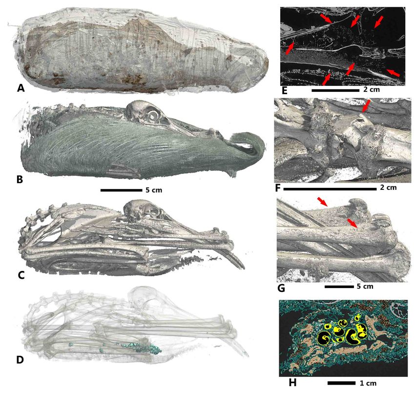
young puppy. Reconstruction of MHNGr.ET.1456 (ibis) is shown in Fig 12. The
ASEMI segmenter with the neural network classifier is used for the general 3D render.
The U-Net segmentations was used to image the feathers and the skeleton, as well as
the gastropods present inside the stomach of the bird. Using the ASEMI segmenter
with the neural network classifier, it was possible to render the neck of the bird,
highlighting twisting of the neck and a broken vertebra. The ASEMI segmenter also
renders detail of the forelimbs showing osteoporosis. All the segmentations raise
questions about the health of the ibis inside the mummy. This can be illustrated by the
fact that the cervical fracture may correspond to the cause of the death of the bird. For
MG.2038 (ibis in a jar), reconstructions are shown in Fig 13. The ASEMI segmenter
with random forest classifier is used for the render of the container. The U-Net
segmenter is used to show the interior, by rendering the jar itself transparently. The
ASEMI segmenter is used to show the textiles, soft parts, and bones. These different
images have brought knowledge on the ibis mummy but also on the jar that contained
it. The jar was made on a wheel rotating clockwise and was sealed with a cover glued
with a mortar. Tomographic data from mummy MHNGr.ET.1017 have shown that the
mummy does not contain a complete bird raptor but only its head stuck on the
wrapped mummy and fixed through a vegetal stem as well as a very juvenile sea bird on
the centre of the fabrics. However, due to the focusing on the internal part of the
mummy, the different segmentations show mainly different type of tissues soaked with
balm, which make the rendering very confusing for non-specialist eyes.
Conclusions
In the Automated SEgmentation of Microtomography Imaging (ASEMI) project we
have developed a tool to automatically segment volumetric images of Egyptian
mummies, obtained using Propagation Phase Contrast Synchrotron Microtomography
(PPC-SRµCT). In contrast to emerging commercial solutions, our tool uses simple 3D
features and classical machine learning models, for a much lower theoretical complexity.
Indicative results were given for four specimens, showing similar overall accuracy when
compared with manual segmentations (94–98% as compared with 97–99% for deep
learning). A qualitative analysis was also given, showing that our results are close in
term of usability to those from deep learning. The output segmentations require some
postprocessing to smoothen noisy edges. Preliminary work using a Markov Random
Field gave promising results, and we plan to implement this in a scalable way.
May 17, 2021 22/28Fig 11. Rendering of the mummy MHNGr.ET.1023 (dog). A: external aspect of the remaining bandages (segmentation ASEMI NN), B: rendering of the preserved soft parts of the puppy (segmentation ASEMI NN), C: rendering of the bones (segmentation U-Net), D: detail on the soft parts showing its weak preservation state through holes certainly from pests or putrefaction (segmentation U-Net), E: rendering of the decidual and permanent dentition of puppy showing its young age (segmentation U-Net). May 17, 2021 23/28
Fig 12. Mummy MHNGr.ET.1456 (ibis). A: general 3D rendering (segmentation ASEMI NN), B: 3D rendering of
feathers of the ibis (segmentation U-Net), C: 3D rendering of the skeleton (segmentation U-Net), D: 3D rendering of the
gastropods (segmentation U-Net), E: virtual slide showing the pest infestation inside the mummy, F: 3D rendering of the
broken vertebra and the twist of the neck (ASEMI NN), G: 3D rendering of the osteoporosis on the forelimbs (ASEMI NN),
H: virtual slide of the stomach (orange highlight) and the gastropods (yellow highlight) (segmentation U-Net).

May 17, 2021                                                                                                     24/28
Fig 13. 3D rendering of the mummy MG.2038 (ibis in a jar). A: general rendering of the external aspect of the
mummy (segmentation ASEMI RF), B: internal content of the mummy made visible thanks to the transparency of the sealed
jar (segmentation U-Net), C: focus on the textile surrounding the animal (segmentation ASEMI RF), focus on the ibis inside
the mummy D: showing its soft part (segmentation ASEMI NN), E: showing the ibis bones (segmentation ASEMI RF).

May 17, 2021                                                                                                        25/28
Acknowledgment
               This project has received funding from the ATTRACT project funded by the EC under
               Grant Agreement 777222. Authors thank Alessandro Mirone for the initial GPU
               implementation of the 3D histogram algorithm, and Andy Götz for project management
               support. We would like to acknowledge the Museum d’Histoire Naturelle de Grenoble
               (France), in particular Philippe Candegabe, for the opportunity to scan the mummies
               MHNGr.ET.1017, MHNGr.ET.1023, MHNGr.ET.1456. We also want to thank the
               Musée de Grenoble (France) in the person of Valérie Huss for providing access to the
               sealed jar MG.2038.

               References
                  1. Berruyer C, Porcier SM, Tafforeau P. Synchrotron “virtual archaeozoology”
                     reveals how Ancient Egyptians prepared a decaying crocodile cadaver for
                     mummification. PLOS ONE. 2020;15(2):e0229140.
                     doi:10.1371/journal.pone.0229140.
                  2. Porcier SM, Berruyer C, Pasquali S, Ikram S, Berthet D, Tafforeau P. Wild
                     Crocodiles Hunted to Make Mummies in Roman Egypt: Evidence from
                     Synchrotron Imaging. Journal of Archaeological Science. 2019;110:105009.
                     doi:10.1016/j.jas.2019.105009.

                  3. Kavur AE, Gezer NS, Barış M, Aslan S, Conze PH, Groza V, et al. CHAOS
                     Challenge – combined (CT-MR) healthy abdominal organ segmentation. Medical
                     Image Analysis. 2021;69:101950. doi:10.1016/j.media.2020.101950.
                  4. Ronneberger O, Fischer P, Brox T. U-NET: Convolutional Networks for
                     Biomedical Image Segmentation. In: Medical Image Computing and
                     Computer-assisted Intervention (miccai). vol. 9351 of Lncs. Springer; 2015. p.
                     234–241. Available from:
                     http://lmb.informatik.uni-freiburg.de/Publications/2015/RFB15a.
                  5. Hati A, Bustreo M, Sona D, Murino V, Bue AD. Weakly Supervised Geodesic
                     Segmentation of Egyptian Mummy CT Scans. CoRR. 2020;abs/2004.08270.

                  6. O’Mahoney T, Mcknight L, Lowe T, Mednikova M, Dunn J. A machine learning
                     based approach to the segmentation of micro CT data in archaeological and
                     evolutionary sciences. bioRxiv. 2020;doi:10.1101/859983.
                  7. Friedman SN, Nguyen N, Nelson AJ, Granton PV, MacDonald DB, Hibbert R,
                     et al. Computed Tomography (CT) Bone Segmentation of an Ancient Egyptian
                     Mummy A Comparison of Automated and Semiautomated Threshold and
                     Dual-Energy Techniques. Journal of Computer Assisted Tomography.
                     2012;36(5):616–622. doi:10.1097/rct.0b013e31826739f5.
                  8. Object Research Systems (ORS). Dragonfly; 2020. Available from:
                     https://www.theobjects.com/dragonfly/index.html.

                  9. Automated segmentation of microtomography imaging of Egyptian mummies;
                     2021. Available from: http://paleo.esrf.eu/.
                 10. ASEMI Segmenter; 2021. Available from:
                     https://github.com/um-dsrg/ASEMI-segmenter.

May 17, 2021                                                                                    26/28
11. Ojala T, Pietikäinen M, Harwood D. A Comparative Study of Texture Measures
with Classification Based on Featured Distributions. Pattern Recognition.
1996;29(1):51–59. doi:10.1016/0031-3203(95)00067-4.
12. Zhao G, Pietikainen M. Dynamic Texture Recognition Using Local Binary
Patterns with an Application to Facial Expressions. IEEE Transactions on
Pattern Analysis and Machine Intelligence. 2007;29(6):915–928.
doi:10.1109/tpami.2007.1110.
13. Abbasi S, Tajeripour F. Detection of brain tumor in 3D MRI images using local
binary patterns and histogram orientation gradient. Neurocomputing.
2017;219:526–535. doi:10.1016/j.neucom.2016.09.051.
14. Barkan O, Weill J, Wolf L, Aronowitz H. Fast High Dimensional Vector
Multiplication Face Recognition. In: 2013 IEEE International Conference on
Computer Vision; 2013. p. 1960–1967.
15. Lowe DG. Object Recognition from Local Scale-invariant Features. In:
Proceedings of the Seventh IEEE International Conference on Computer Vision.
vol. 2. IEEE; 1999. p. 1150–1157.
16. Bay H, Ess A, Tuytelaars T, Van Gool L. Speeded-Up Robust Features (SURF).
Computer Vision and Image Understanding. 2008;110(3):346 – 359.
doi:https://doi.org/10.1016/j.cviu.2007.09.014.
17. Tin Kam Ho. The random subspace method for constructing decision forests.
IEEE Transactions on Pattern Analysis and Machine Intelligence.
1998;20(8):832–844. doi:10.1109/34.709601.
18. Pedregosa F, Varoquaux G, Gramfort A, Michel V, Thirion B, Grisel O, et al.
Scikit-learn: Machine Learning in Python. Journal of Machine Learning Research.
2011;12:2825–2830.
19. Bishop CM. Neural Networks for Pattern Recognition. USA: Oxford University
Press, Inc.; 1995.
20. Abadi M, Agarwal A, Barham P, Brevdo E, Chen Z, Citro C, et al.. TensorFlow:
Large-Scale Machine Learning on Heterogeneous Systems; 2015. Available from:
https://www.tensorflow.org/.
21. Cristianini N, Shawe-Taylor J. An Introduction to Support Vector Machines and
Other Kernel-based Learning Methods. Cambridge University Press; 2000.
22. NVIDIA CUDA C Programming Guide; 2018.
23. Çiçek Ö, Abdulkadir A, Lienkamp SS, Brox T, Ronneberger O. 3D U-Net:
Learning Dense Volumetric Segmentation from Sparse Annotation. In: Ourselin
S, Wells WS, Sabuncu MR, Unal G, Joskowicz L, editors. Medical Image
Computing and Computer-Assisted Intervention (MICCAI). vol. 9901 of LNCS.
Springer; 2016. p. 424–432. Available from:
http://lmb.informatik.uni-freiburg.de/Publications/2016/CABR16.
24. Mirone A, Brun E, Gouillart E, Tafforeau P, Kieffer J. The PyHST2 hybrid
distributed code for high speed tomographic reconstruction with iterative
reconstruction and a priori knowledge capabilities. Nuclear Instruments and
Methods in Physics Research Section B: Beam Interactions with Materials and
Atoms. 2014;324:41–48. doi:10.1016/j.nimb.2013.09.030.
May 17, 2021 27/2825. Paganin D, Mayo SC, Gureyev TE, Miller PR, Wilkins SW. Simultaneous phase
and amplitude extraction from a single defocused image of a homogeneous object.
Journal of Microscopy. 2002;206(1):33–40. doi:10.1046/j.1365-2818.2002.01010.x.
May 17, 2021 28/28You can also read