Impact of high- and low-vorticity turbulence on cloud-environment mixing and cloud microphysics processes
←
→
Page content transcription
If your browser does not render page correctly, please read the page content below
Atmos. Chem. Phys., 21, 12317–12329, 2021
https://doi.org/10.5194/acp-21-12317-2021
© Author(s) 2021. This work is distributed under
the Creative Commons Attribution 4.0 License.

Impact of high- and low-vorticity turbulence on cloud–environment
mixing and cloud microphysics processes
Bipin Kumar1 , Rahul Ranjan1,2 , Man-Kong Yau3 , Sudarsan Bera1 , and Suryachandra A. Rao1
1 IndianInstitute of Tropical Meteorology, Ministry of Earth Sciences, Pashan, Pune 411008, India
2 Department  of Atmospheric and Space Science, Savitribai Phule Pune University, Pune 411007, India
3 Department of Atmospheric and Ocean Science, McGill University, Montréal, Quebec H3A 0B9, Canada

Correspondence: Bipin Kumar (bipink@tropmet.res.in)

Received: 2 February 2021 – Discussion started: 18 March 2021
Revised: 24 June 2021 – Accepted: 14 July 2021 – Published: 17 August 2021

Abstract. Turbulent mixing of dry air affects the evolution of          1   Introduction
the cloud droplet size spectrum via various mechanisms. In a
turbulent cloud, high- and low-vorticity regions coexist, and
inertial clustering of cloud droplets can occur in low-vorticity
regions. The nonuniformity in the spatial distribution of the           Clouds are a visible manifestation of tiny water droplets
size and in the number of droplets, variable vertical veloc-            or ice crystals in the Earth’s atmosphere. They play mul-
ity in vortical turbulent structures, and dilution by entrain-          tiple roles in atmospheric processes, ranging from the ra-
ment/mixing may result in spatial supersaturation variability,          diation budget to the hydrological cycle (Bengtsson, 2010;
which affects the evolution of the cloud droplet size spectrum          Grabowski and Petch, 2009; Harrison et al., 1990; Randall
via condensation and evaporation processes. To untangle the             and Tjemkes, 1991). The size of clouds may extend from
processes involved in mixing phenomena, a 3D direct nu-                 a few meters to several kilometers. However, the suspended
merical simulation of turbulent mixing followed by droplet              droplets that constitute a cloud are much smaller – with a
evaporation/condensation in a submeter-sized cubed domain               typical radius of 1–20 µm. The journey from a cloud droplet
consisting of a large number of droplets was performed in               to a raindrop (∼ 103 µm) is a complicated process. Conden-
this study. The analysis focused on the thermodynamic and               sation and collision–coalescence, the two key processes in-
microphysical characteristics of the droplets and the flow in           volved in the growth of a droplet, are prominent at differ-
high- and low-vorticity regions. The impact of vorticity gen-           ent stages of cloud development (Rogers and Yau, 1996).
eration in turbulent flows on mixing and cloud microphysics             For example, up to a size of 15 µm, diffusional-condensation
is illustrated.                                                         growth dominates, whereas collision–coalescence is effec-
                                                                        tive when the droplet radius reaches approximately 40 µm
                                                                        (Pruppacher and Klett, 1997). The rapid growth of droplets
                                                                        in the size range between 15 and 40 µm – for which neither
Highlights.                                                             condensational growth nor collision–coalescence is effective
  – Regions of high vorticity are prone to homogeneous mixing           – is poorly understood. This size range has been termed
    due to faster mixing by air circulation.                            the “condensation–coalescence bottleneck” or the “size gap”
  – The microphysical droplet size distribution is wider or nar-        (Grabowski and Wang, 2013). The rapid growth of droplets
    rower in high- or low-vorticity volumes, respectively.              in the size gap is regarded as one of the important unresolved
  – Drier environmental air mixing initially leads to a higher spec-    problems in cloud physics. To explain the rapid growth, sev-
    tral width.                                                         eral mechanisms like entrainment, turbulent supersaturation
  – The k-means clustering algorithm (an unsupervised machine           fluctuations, enhanced collision rates due to turbulence, and
    learning technique) is used to identify regions of high vorticity   the role of giant aerosols have been proposed. This study fo-
    in the computational domain.                                        cuses on the interaction between droplets and turbulence to

Published by Copernicus Publications on behalf of the European Geosciences Union.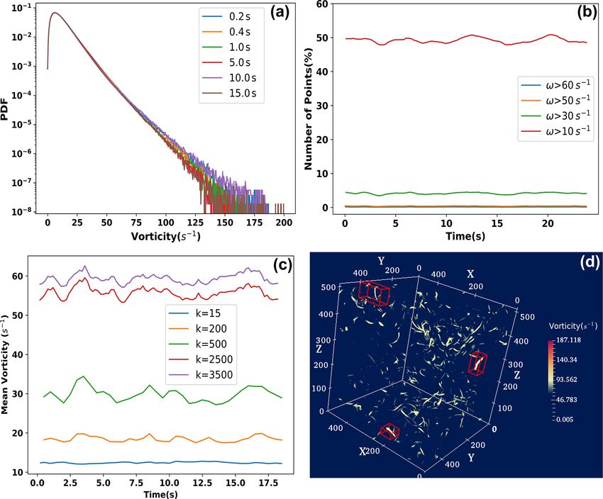
12318                                                              B. Kumar et al.: Impact of vorticity on cloud turbulence

explore how this interaction modifies the droplet characteris-     bution. However, Grabowski and Vaillancourt (1999) com-
tics.                                                              mented on the limitations of applying the results of Shaw et
                                                                   al. (1998) to atmospheric clouds due to the absence of droplet
1.1   Role of turbulence in cloud microphysics                     sedimentation, the assumption of the high volume fraction of
                                                                   vortex tubes (50 %), and the strong dependence on the vortex
Understanding the impact of turbulence on the dynamics and         lifetime.
microphysics of clouds is a long-standing problem (Devenish           There is no clear theory regarding vorticity characteristics
et al., 2012; Grabowski and Wang, 2013; Khain et al., 2007;        in 3D homogeneous turbulent flows, despite increasing re-
Shaw, 2003; Vaillancourt and Yau, 2000) and has been an            search on turbulence. Vorticity has a profound impact on the
active area of research using in situ observations and numer-      spatial distribution of droplets. Due to preferential cluster-
ical models. The position and movement of droplets are con-        ing, relatively fewer droplets are left in high-vorticity regions
trolled by turbulent eddies of varying sizes. Simultaneously,      (Karpińska et al., 2019). The difference in the spatial distri-
evaporation or condensation of droplets incurs changes in the      bution of droplets induces supersaturation fluctuations. The
local environment (∼ scale of droplet itself) through latent       low number of droplets competing for the available vapor
heat exchange. Additionally, buoyancy generated by phase           field in high-vorticity regions should experience enhanced
change (when a bunch of droplets evaporate or condense in-         growth. However, for this to happen, droplets should stay in
stead of a few) may impact cloud-scale motions. The inertial       these regions for a duration long enough for the supersatura-
response time “τp ” is a quantity that determines how quickly      tion field to act. In general, little is known about the spatial
droplets respond to changes in the surrounding fluid motion        scale and lifetime of high-vorticity regions (Grabowski and
(Clift et al., 1978). Some droplets are tiny and precisely fol-    Wang, 2013). Due to these limitations, the effect of preferen-
low the flow trajectory, whereas larger droplets can modify        tial clustering on the diffusional growth of droplets is poorly
the flow. Thus, droplet–turbulence interaction is a multiscale     understood.
process and is nonlocal in nature.                                    In this study, we examine the diffusional growth and evap-
   There are several macrophysical and microphysical im-           oration of cloud droplets in an entrainment and mixing sce-
plications of droplet–turbulence interactions. Droplets in the     nario using direct numerical simulation (DNS). We com-
decaying part of a cloud may be transported by turbulence          pare the droplet characteristics, such as spectral width, vol-
to the more active regions to undergo further growth (Baker        ume mean radius, number concentration, probability density
and Latham, 1979; Jonas, 1991). The inhomogeneous mix-             function (PDF) of droplet radii, and supersaturation, in high-
ing model used by Cooper et al. (1986) and Cooper (1989)           and low-vorticity regions. As reported by Vaillancourt et al.
shows that when a parcel of air undergoes successive entrain-      (1997), the main entrainment sites and mixing zones were
ment events, each of which reduces the droplet concentra-          located in the vortex circulation areas. Accordingly, using
tion, it can lead to enhanced droplet growth. However, Jonas       DNS, we aim to look for locations with vortex circulations
(1996) argues that ascent leading to droplet growth may acti-      in the main entrainment sites and mixing zones. In sum-
vate some entrained nuclei to limit the maximum supersatu-         mary, the main purpose of this study is to seek answers to
ration achieved which, in turn, limits the droplet growth rate.    the questions regarding the volume fraction of high-intensity
Vaillancourt et al. (1997) gives further insight into the nature   vortices in a turbulent domain and the dominant locations of
of turbulent entrainment at the cloud edges. They argue that       mixing in the high- and low-vorticity regions. Thus, the spe-
the interaction between the ambient and the cloudy air is not      cific scientific considerations in this work are (i) variations in
the same everywhere. There are some prominent regions of           droplet spectral properties in high- and low-vorticity regions,
entrainment with vortex circulations.                              (ii) quantification of the degree of mixing in these regions,
   The study of microphysical droplet–turbulence interac-          and (iii) the impact of relative humidity on the evolution of
tion has gained momentum in recent years due to advances           the droplet size spectra.
in computational capabilities. Several possibilities such as          The organization of the paper is as follows: Sect. 2 pro-
turbulence-induced supersaturation fluctuation and enhanced        vides details of the methods and data used; results and dis-
collision rates have been investigated. Some studies (Chen et      cussions are provided in Sect. 3, with further four subsections
al., 2016; Franklin et al., 2005; Pinsky et al., 2000; Riemer      containing the discussion of the flow and the droplet charac-
and Wexler, 2005; Shaw, 2003; Vaillancourt and Yau, 2000)          teristics in low- and high-vorticity regions; and we concluded
indicate an enhanced collision rate in a turbulent environ-        our findings in Sect. 4.
ment. Shaw et al. (1998) performed a model simulation with
a Rankine vortex and found that the preferential clustering of
droplets in the low-vorticity regions increases the spatially      2   Data and methods
varying supersaturation. On the other hand, droplets in the
high-vorticity regions experience enhanced supersaturation         We carried out a DNS following the setup of Kumar et
and grow faster. This work laid the foundation for droplet         al. (2014, 2018) to simulate the entrainment and mixing
clustering in clouds and its effect on the droplet size distri-    mechanisms at cloud edges. This DNS code uses the Euler–

Atmos. Chem. Phys., 21, 12317–12329, 2021                                           https://doi.org/10.5194/acp-21-12317-2021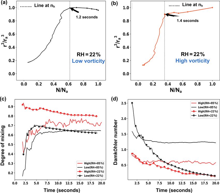
B. Kumar et al.: Impact of vorticity on cloud turbulence                                                                     12319

Lagrangian framework, solves the flow equations at each grid       dataset; instead, the user has to assign it. Therefore, selecting
point, and tracks each droplet inside a grid by integrating        the number of groups or clusters in which a dataset has to be
the equations for its position, velocities, and growth rate.       grouped or clustered is crucial. This algorithm was used to
The simulation produces the output in two formats: one is          locate high-vorticity regions from the vorticity data.
from the Eulerian framework in NetCDF format developed                The absolute vorticity ω related to the velocity compo-
by UCAR/Unidata, and the other is the droplet dynamics out-        nents is calculated as follows (see Sect. 4.2 in Holton and
put saved in SION format (SIONLib, 2020). The simulation           Hakim, 2013):
domain was chosen (51.2 cm)3 with a 1 mm grid resolution                                1
and, thus, contained a total of (512)3 grid points in the do-      ω = ωi2 + ωj2 + ωk2 ,
                                                                                          2
                                                                                                                                 (1)
main. An initial setup of the computational domain is de-
tailed in Sect. 3.                                                 where
   Two simulation setups are considered in this study. In par-            δw δv               δu δw               δv δu
ticular, there are two relative humidity (RH) cases (85 % and      ωi =      − ;       ωj =      −    ;    ωj =     − .         (2)
                                                                          δy  δz              δz   δx             δx δy
22 %) initialized with a polydisperse droplet size distribution.
We also attempted two simulations (two RH cases) initial-              The values of ω range from 0 to 200 s−1 in our DNS data,
ized by a monodisperse droplet size (20 µm). However, our          as seen in Fig. 1a. Vaillancourt and Yau (2000) mentioned
discussion is focused only on the results from the polydis-        that only a small fraction of the cloud core is occupied by
perse case as the monodisperse case does not provide any ad-       high-vorticity regions, and no preferential concentration of
ditional results. The polydisperse setup contains the droplet      cloud droplet was observed there. We also found that less
size distribution (size range 2–18 µm) from cloud observa-         than 2 % of the grids (by volume) have a vorticity with a
tions (Cloud Aerosol Interaction and Precipitation Enhance-        magnitude greater than 60 s−1 . For larger vorticity magni-
ment Experiment – CAIPEEX: https://www.tropmet.res.in/             tudes, even fewer grids (an almost negligible number) were
~caipeex/, last access: 11 August 2021) used in Kumar et           located. Based on these findings a threshold value of vorticity
al. (2017) with a mean radius of 9.3 µm. The two humid-            magnitude of 60 s−1 was chosen as the high-vorticity crite-
ity levels, corresponding to dry (RH = 22 %) and moist air         rion in this work. We also investigated the droplets’ charac-
(RH = 85 %), were taken from observations of the monsoon           teristics with a threshold of 50 s−1 , but the trends showed no
environment (Bera et al., 2016). A supersaturated cloudy slab      difference. We also mention that using 30 s−1 as a threshold
in the DNS domain is specified to simulate the mixing pro-         for high vorticity, which is less than one-fifth of the maxi-
cesses.                                                            mum vorticity magnitude (200 s−1 ), does not seem to be jus-
   This study aims to investigate droplet characteristics in       tified. Figure 1b depicts the fraction of grid points for differ-
high- and low-vorticity regions in cloud turbulence. There-        ent threshold values of vorticity magnitude.
fore, the vorticity magnitudes were first calculated using the         Once the threshold value for vorticity magnitude is de-
Eulerian data at each grid point containing the velocity com-      cided, the next step is to locate 3D boxes enclosing the high-
ponents in the x, y and z directions. The next step is to find     vorticity regions. We look for these regions at every time
the high- and low-vorticity regions in the DNS computational       step. To locate the boxes with high vorticity, we applied a ma-
domain. This requires calculating and visualizing the actual       chine learning algorithm, namely, k-means clustering. When
vortices generated by the turbulent flow. As the grid size is      using this algorithm, two input variables have to be assigned
1 mm, it is not feasible to obtain a vortex inside a single grid   a value: (i) the number of clusters (“k”) and (ii) the maxi-
box; instead, a volume containing the vortex must be sought,       mum number of iterations. As vortices have tubular or sheet-
encompassing multiple grid boxes. It is a challenging task         like structures, it is possible that a 3D box may contain many
to locate a small box to cover a minimal portion of the low-       low-vorticity points for a typical value of k. Hence, an opti-
vorticity region. We used an unsupervised machine learning         mal value of k is required to select small enough 3D boxes to
(ML) algorithm (mentioned in the next subsection) to address       avoid the low-magnitude vorticity points.
this problem.                                                          We identified the value of k to be used in the algorithm
                                                                   by conducting several experiments and selected the optimal
2.1   Locating high-vorticity regions                              value k = 3500 based on the chosen threshold value for high
                                                                   vorticity. At k = 3500, the average vorticity in the boxes
To locate high-vorticity regions in the domain, we used the        reaches close to the selected threshold (60 s−1 ), as shown in
k-means clustering algorithm from the “scikit-learn” Python        Fig. 1c. This figure provides the vorticity values for different
package (Pedregosa, 2011). k-means clustering (Bock, 2007)         values of k and confirms the appropriate choice of k = 3500.
is one of the most popular and the simplest unsupervised           The value of k also affects the size of the cluster. With an in-
machine learning algorithms. It makes “k” groups or clus-          creasing value of k, the size of the clusters decreases. Conse-
ters from a dataset based on the Euclidean distance between        quently, some clusters may become so small that they might
individual data points. However, k-means clustering can-           only include as many as approximately two or three high-
not guess the optimum number of clusters for a particular          vorticity points, which are all in the same plane. These points

https://doi.org/10.5194/acp-21-12317-2021                                        Atmos. Chem. Phys., 21, 12317–12329, 2021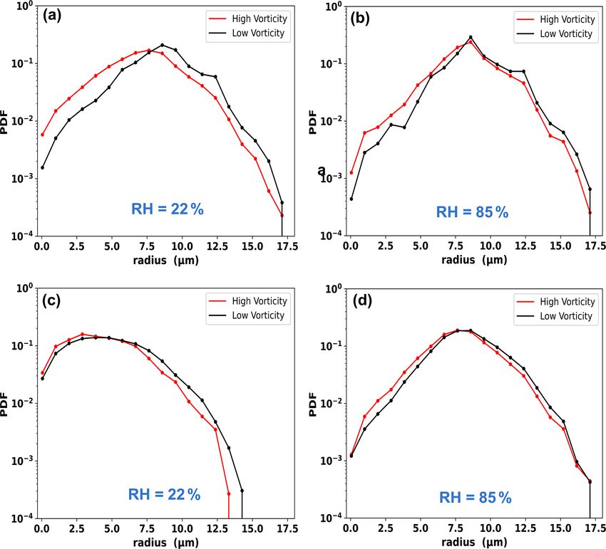
12320                                                                       B. Kumar et al.: Impact of vorticity on cloud turbulence

Figure 1. Panel (a) displays the probability density function (PDF) of vorticity at different times. The fraction of high-vorticity points (based
on threshold values) are depicted in panel (b). Panel (c) represents vorticity values for different values of k. Panel (d) shows high-vorticity
regions (enclosed by a rectangular cuboid) obtained for k = 500.

in the same plane will not be useful, as they cannot form a                at small spatial scales and that a low (high) particle concen-
cuboid. Therefore, the k = 3500 value was found to be op-                  tration corresponds to high (low) vorticity regions using a
timal. For a higher value of k, we may get many zero vol-                  Rankine vortex in their model. They assumed a high fraction
ume boxes. That is the reason why increasing the value of k                (50 %) of vortex structure and that the preferential concentra-
indefinitely is not advisable. Similarly, the optimal numbers              tion of droplets was severalfold higher than the mean droplet
of iterations were chosen as 200 to keep the computational                 concentration. In contrast, the high-vorticity region in the
cost moderate. A typical visualization of finding a volume                 present simulation is very small (≈ 0.2 % volume fraction)
enclosing a high-vorticity region is shown in Fig. 1d, where a             with a droplet concentration that is about 1.5-fold higher than
cuboid is shown to surround the high-vorticity region. It was              in the low-vorticity region.
noted that high-vorticity regions occupy only a tiny fraction                 A comparison of the methods in this work and the study of
(0.1 %–0.2 %) of the total domain.                                         Shaw et al. (1998) is provided in Table 1. For calculating the
   This finding of a tiny fraction for high-vorticity regions              volume fraction of a high-vorticity region, Shaw et al. (1998)
in a cloud core is in agreement with the DNS study of                      considered two zones of vortices (high and low vorticity) in
Jimenez et al. (1993) and Vaillancourt and Yau (2000) but                  their parcel model with a Rankine vortex and considered the
disagrees with the assumed high volume fraction (≈ 50 %)                   same volume fraction (i.e., 50 %) for the two vorticity zones.
from Squires and Eaton (1991) and later from Shaw et al.
(1998). There are important differences between this study
and the study of Shaw et al. (1998), who laid the foundation               3   Results and discussion
of inertial clustering of cloud droplets and motivated us to
conduct the present study. Shaw et al. (1998) hypothesized                 In this section, we discuss the various analyses from the two
that the preferential concentration (inertial clustering) occurs           humidity simulations initialized with a polydisperse droplet
                                                                           size spectrum.

Atmos. Chem. Phys., 21, 12317–12329, 2021                                                    https://doi.org/10.5194/acp-21-12317-2021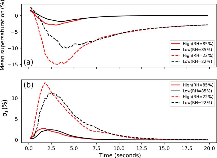
B. Kumar et al.: Impact of vorticity on cloud turbulence                                                                                12321

Table 1. A comparison of this study with the previous study of Shaw et al. (1998) that laid the foundation for droplet clustering and its impact
on the droplet size distribution. Kolmogorov timescales in natural clouds are in the range of 0.01–0.1 s. The Kolmogorov timescale for DNS
is 0.0674 s, which lies in the above mentioned range.

               Setup                                 Shaw et al. (1998)                                              This study
               Entrainment mixing                    No                                                              Yes
               Vortex lifetime                       2–3 orders of magnitude > Kolmogorov timescale (≈ 10 s)         < 1s
               Volume fraction of high vorticity     ≈ 50 %                                                          < 2%

Figure 2. A snapshot of the DNS domain at a time of 0.2 s, which          Figure 3. Panel (a) shows the variation in kinetic energy (KE) for
can be considered as the initial state of the simulation. The figure      both the drier and humid cases in the cloudy slab and edges. Mean
also shows two boxes at the edges (left and right white boxes) and        vorticity variations at the edges and within the cloudy slab (for both
the initial cloud slab (central black box). The legend represents the     cases) are shown in panel (b). The KE was averaged over the cloudy
fluctuation from the mean temperature.                                    slab and both drier edges. The vorticity average was taken in each
                                                                          box enclosing them.

3.1   Initial simulation setup
                                                                          as depicted in Fig. 3a. The availability of more kinetic energy
The interface between cloud volume and the subsaturated air               at the cloud edges makes them the hot spots for vorticity gen-
is distinguishable during the early evolution of the flow. To             eration. Initially, a higher mean vorticity value is observed at
see if any features of the flow exhibit distinct properties at            the edges in both humidity cases, which is evident in Fig. 3b.
the edges, three separate volumes from the entire domain                  Near the edges, strong gradients of mixing ratio and temper-
have been selected. The cloudy slab area lies between 142                 ature exist, leading to the generation of instabilities and, con-
and 372 mm along the x axis, with the rest of the domain oc-              sequently, turbulent mixing. Turbulent kinetic energy (TKE)
cupied by the subsaturated air. Of the two interface volumes,             is initially associated with the vortical motions at the inter-
one is on the left side (between x = 70 and 140 mm), and the              face; however, additional TKE is also generated due to neg-
other is on the right side (between x = 364 and 434 mm). The              ative buoyancy production by droplet evaporation. This en-
volume lying between x = 182 and 322 mm is in the core re-                ergy is transported to the cloud slab as time progresses by
gion, as depicted in Fig. 2.                                              the vortices (“eddies”) that propagate inward. However, there
                                                                          are periodic changes in the TKE variations between the inter-
3.2   Turbulence characteristics at the edges and core of                 face and the cloud slab that are possibly due to the periodic
      cloud                                                               boundary condition of the DNS setup. A notable feature be-
                                                                          tween the two RH simulations (22 % and 85 %) is the larger
The cloudy volume properties initially see sharp changes,                 difference in vorticity between the interface and the cloud
which were confirmed by analyzing the variations in kinetic               slab in the drier case (RH = 22 %) due to the strongest evap-
energy (KE), vorticity and mixing ratio. The edges are the                oration.
most turbulent part of the clouds during early evolution, and
considerable robust fluctuations in KE are experienced there,

https://doi.org/10.5194/acp-21-12317-2021                                                 Atmos. Chem. Phys., 21, 12317–12329, 2021
12322 B. Kumar et al.: Impact of vorticity on cloud turbulence
3.3 Flow characteristics in high- and low-vorticity dius. Consequently, the number concentration curves almost
regions merge after 7.5 s. Due to preferential clustering, the high-
vorticity regions have a relatively small number of droplets.
The previous subsection presented the variation in flow char- It is to be noted that the low-vorticity region always has a
acteristics at the cloud core and the edges. Another part of larger mean volume radius during the simulations, as shown
this study is to investigate these characteristics in the high- in Fig. 5b.
vorticity (HV) regions of the turbulent flow, with a vorticity There may be two possible reasons for the smaller value
magnitude greater than 60 s−1 . Similarly, points with vortic- of the mean radius in high-vorticity regions: (i) droplets ex-
ity less than 30 s−1 were classified as regions of low vorticity perience a drier environment and evaporate faster during the
(LV). early stage of mixing when high vorticity forms at the cloud
We also investigated the evolution of the vapor mixing ra- edge, and (ii) larger droplets are more likely to be flung out of
tio (qv ) in both the drier (RH = 22 %) and the more humid the high-vorticity region as a consequence of a greater inertia
cases (RH = 85 %). The incursion of drier air results in a effect, leaving behind only the smaller droplets (i.e., prefer-
lower mixing ratio at the edges, as evident from Fig. 4a. In ential clustering is more prominent for larger droplets). The
both the HV and LV regions, we further determined the root second possibility is more valid during the later part of the
mean square velocity Urms . For the dry and humid cases, simulation (approx. after 5 s) when high vorticity forms in-
Urms is found to be higher in HV regions as depicted in side the cloud slab. To clarify whether preferential cluster-
Fig. 4a. ing alone determines the volume mean radius distribution or
whether the other mechanisms are responsible, we investi-
3.4 Droplet characteristics gated the droplet spectra, the trends of the mean supersatura-
tions and the evolution of the droplet size distribution.
One of the main aims of this study is to examine various
droplet characteristics, such as number concentration, vol- 3.4.2 Evolution of droplet size spectra
ume mean radius, spectral width, and the mixing process in
HV and LV regions. This subsection focuses on all of these The variation in the spectral width is presented in Fig. 6a,
characteristics. showing an entirely different picture of the evolution of
droplet spectra in the two cases. Figure 6b illustrates the dis-
3.4.1 Number concentration and mean volume radius persion of the droplet size distribution (DSD).
During the initial mixing of the cloud slab with the envi-
There have been many kinds of research on the distribution ronmental dry air in the RH = 22 % case, the spectral width
of droplets in a turbulent flow field. Several laboratory stud- of the DSD increases rapidly until the 5–7 s mark and then
ies (Lian et al., 2013) and model simulations (Shaw et al., decreases thereafter, whereas in the RH = 85 % case, a grad-
1998; Ayala et al., 2008) reported on the process of prefer- ual increase can be seen for the initial 10 s and remains al-
ential clustering of cloud droplets in low-vorticity regions. most constant after that. One of the most important results
The preferential clustering means that droplets prefer to clus- of this study is that the spectral width of the DSD is differ-
ter in some specific flow regions rather than randomly dis- ent in high- and low-vorticity regions, as depicted in Fig. 6.
tributed everywhere. A high amount of rotation characterizes The droplet size dispersion also confirms that the broaden-
the highly vortical part of a fluid. When a droplet enters this ing is always stronger in the high-vorticity regions. For the
region, it is flung out due to its inertia and accumulates in a RH = 22 % case, the spectral width is wider for droplets sit-
low-vorticity region. uated in a high-vorticity region during the initial 5 s of mix-
This process leads to a heterogeneous droplet concentra- ing when the spectral width increases rapidly. However, the
tion in space – an important aspect that affects the droplet opposite scenario occurs after 7.5 s (i.e., narrower spectral
growth rate and the size distribution. In a polydisperse size width in high-vorticity regions). Nevertheless, the spectral
distribution, the larger droplets are more prone to be affected width is always wider in the high-vorticity regions in the
by the vorticity compared with smaller droplets that may fol- RH = 85 % case.
low the flow streamline due to their low inertia. For this rea- The initial growth and later decay of the spectral width
son, larger droplets accumulate in low-vorticity regions and during mixing for the RH = 22 % case is associated with the
result in a larger mean volume radius. modification of the spectral shape by droplet evaporation and
In Fig. 5a, both humidity cases show almost the same trend the number concentration dilution (see Bera, 2021). In this
(i.e., a higher number concentration in the low-vorticity re- case, evaporation is very significant due to the mixing of the
gion due to inertial clustering). Figure 5b shows the variation much drier environmental air. When evaporation starts, the
in the mean volume radius in high- and low-vorticity regions. smaller droplets of the DSD evaporate faster than the larger
The arid-like conditions in the case with RH = 22 % leads to droplets in accordance with the inverse relation of growth
fast evaporation of droplets, as indicated by the rapid decay rate with droplet size (Rogers and Yau, 1996). As a result,
in the droplet number concentration and the mean volume ra- the spectra shift towards the smaller size tail, as shown in
Atmos. Chem. Phys., 21, 12317–12329, 2021 https://doi.org/10.5194/acp-21-12317-2021B. Kumar et al.: Impact of vorticity on cloud turbulence 12323
Figure 4. The evolution of the vapor mixing ratio is depicted in panel (a). Panel (b) represents the variation in Urms .
Fig. 7. This is the reason for the increasing spectral width
for the initial 5 s in RH = 22 % and during the entire 20 s
of RH = 85 %. However, when evaporation is such that the
smaller size tail of the spectra is evaporated completely and
only larger droplets remain, the spectra start to shrink and the
spectral width decreases, as shown in Fig. 7c (see Luo et al.,
2020). This is the situation for RH = 22 % with mixing after
7.5 s but does not occur for RH = 85 % case where the evap-
oration is much slower due to moist air mixing (as shown in
Fig. 7d).
The difference in the spectral width in the HV and LV re-
gions can be identified by the higher droplet evaporation in
high-vorticity regions. Initially, high vorticity forms at the
cloud edges where dry air mixing occurs, leading to faster
evaporation of droplets. A second possibility is that high-
vorticity regions are pockets of rotating air motions that can
easily transport the vapor mass (produced by droplet evapo-
ration) out of the region to facilitate enhanced evaporation.
These two plausible reasons result in higher evaporation rate
in regions of high vorticity and, consequently, impact of the
droplet spectral width.
The differences in the PDFs of HV and LV regions are very
noticeable at 3 and 17.8 s. During this time, a greater spectral
width exists in the high-vorticity region (refer to Fig. 6) for
both humidity cases (i.e., RH = 22 % and RH = 85 %). The
PDFs confirm that high- and low-vorticity regions contain
almost the same maximum and minimum drop sizes, but the
difference comes from the distribution. The following possi-
Figure 5. The evolution of the number concentration (Nd ) in the bilities can explain the characteristics of the PDF depicted:
whole domain is shown in the inset of panel (a). In both RH
cases, initial number densities (in the entire domain) were close to – saturation ratio is lower in high-vorticity regions, which
130 cm−3 . However, as seen in panel (a), the evolution of Nd in triggers enhanced evaporation;
high- and low-vorticity regions has different magnitudes: it is al-
ways greater in the low-vorticity regions. Panel (b) shows the vol- – due to enhanced evaporation, there are smaller droplets
ume mean radius, which is always smaller in the high-vorticity re- in the vortices, as depicted by the size distribution;
gions.
– bigger droplets are more vulnerable to be thrown out of
the vortices, leaving only the smaller ones.
https://doi.org/10.5194/acp-21-12317-2021 Atmos. Chem. Phys., 21, 12317–12329, 202112324 B. Kumar et al.: Impact of vorticity on cloud turbulence Figure 6. The variation in the spectral width in high- and low-vorticity regions is shown in panel (a). The spectral width is always greater in the high-vorticity region in the RH = 85 % case, whereas it is only greater for the initial 5 s in the RH = 22 % case. Panel (b) depicts the variation in the dispersion of the droplet size distribution with time. Figure 7. The probability density function (PDF) of the droplet radii for RH = 22 % (a, c) and RH = 85 % (b, d). Panels (a) and (c) depict the plots for 3 s, and panels (b) and (d) depict the plots for 17.8 s. Atmos. Chem. Phys., 21, 12317–12329, 2021 https://doi.org/10.5194/acp-21-12317-2021
B. Kumar et al.: Impact of vorticity on cloud turbulence 12325
ber concentration are normalized by the respective adiabatic
values (Gerber et al., 2008; Kumar et al., 2014). In a similar
manner, we performed the mixing diagram calculation, and
we depict the values in Fig. 9a and b. Here, we have con-
sidered the initial values (t = 0 s) as adiabatic in the mixing
diagram.
An analysis of the mixing diagrams in the high- and low-
vorticity regions for both the moist and dry cases were per-
formed. Variations in mixing diagrams in high- and low-
vorticity regions for the RH = 22 % case are depicted in
Fig. 9a and b, respectively. The mixing diagrams, for both
RH cases, show a clear picture of mixing types. In the low-
vorticity case, the mixing is inactive up to 1.2 s, whereas for
HV case, it remains inactive up to 1.4 s. During this time,
entrained air just dilutes the number concentration (nh ) with-
out acting on droplet evaporation (because the cloudy slab
Figure 8. Panel (a) shows the evolution of the mean saturation ra- expands during this time and droplets scatter into the entire
tio in the high- and low-vorticity regions. The saturation ratio is
domain). Afterward, physical mixing occurs, the mixing line
lower in the high-vorticity regions during the initial 5–7 s; its value
reaches a minimum of −15 % in the RH = 22 % case, whereas it
takes a turn toward the homogenous mixing line (vertical line
only drops to −3 % in the RH = 85 % case. The evolution of the representing constant number concentration), and both the
standard deviation of the saturation ratio in high- and low-vorticity number density and the mean volume radius decrease rapidly,
regions is shown in panel (b). The standard deviation sees a steeper indicating an intermediate or transient-type mixing scenario.
increase and decrease in high-vorticity regions. It has a large vari- One can summarize that the mixing in HV regions remains
ation (0–14) in the RH = 22 % case, whereas the variation is small more homogeneous compared with LV regions, as can be
(0–2.8) in the RH = 85 % case. seen by the more rapid droplet evaporation (decrease in r)
than the decrease in number density.
The degree of mixing was calculated using the following
For further understanding, we also analyzed the trend of formula from Lu et al. (2012), which is based on a “β” pa-
the droplet supersaturation, as outlined in the following. rameter:
3
3.4.3 Mean saturation ratio r3 − 1
r
β = tan−1 na nh . (3)
Figure 8 depicts the mean and standard deviation of su- n −n
a a
persaturation variation in HV and LV vorticity regions for
the RH = 22 % and RH = 85 % cases. The droplets in high- β is normalized by π/2 to obtain a mixing degree that
vorticity regions experience a comparatively lower satura- varies between [0, 1]. In this equation, r is the mean volume
tion ratio until around 6 s, after which the difference tends radius; ra stands for the adiabatic volume mean radius; and
to vanish. Hence, during the entrainment of drier air into the n, nh and na are the number concentration, homogeneous
cloudy volume, droplets encounter a more subsaturated envi- number concentration and adiabatic number concentration,
ronment in the highly vortical regions, and it is the lower sat- respectively.
uration ratio values that produce a larger standard deviation. The degree of mixing is presented in Fig. 9c. It is calcu-
In the RH = 22 % case, the saturation ratio drops to −15 %, lated using Eq. (3) (Lu et al. , 2012). The values of the degree
whereas in the RH = 85 % case, although a similar pattern are in the range [0, 1]. The value 1 represents homogeneous
exists, the saturation ratio only drops to −3 %. In summary, mixing, and extreme inhomogeneous mixing has a 0 value.
the high-vorticity regions can be identified as zones of en- We observed a higher mixing degree in the HV regions in
trainment. both RH cases. The moist case shows relatively inhomoge-
neous mixing initially for both LV and HV regions and grad-
3.4.4 Degree of mixing ually shifts towards homogeneous mixing, although the HV
region always remains at the higher side of homogeneous
One of the best metrics to investigate the entrainment and mixing.
mixing process is the degree of mixing, which depends on A comparison of Damköhler numbers for all four cases is
the mixing diagram and has a wider application in numeri- presented in Fig. 9d. The Damköhler number also measures
cal models (Lehmann et al., 2009; Kumar et al., 2017, 2018). the degree of mixing as a quantity related to two timescales,
In the mixing diagram, the volume mean radius cube (r 3 ) is namely the fluid timescale (τfluid = L/Urms ) and the phase
plotted against the number concentration (Nd ). Sometimes, a relaxation timescale (τphase = 4πn1d Dr ) (Kumar et al., 2012),
normalized version is plotted, in which the radius and num- where Urms is the root mean square of the turbulent veloc-
https://doi.org/10.5194/acp-21-12317-2021 Atmos. Chem. Phys., 21, 12317–12329, 202112326 B. Kumar et al.: Impact of vorticity on cloud turbulence
Figure 9. Panels (a) and (b) represent the mixing diagrams for the respective low- and high-vorticity regions for the RH = 22 % case. nh
represents the homogeneous number concentration used in Eq. (3). Degrees of homogeneous mixing for all four cases are compared in panel
(c). A comparison of the Damköhler number for all the cases is shown in panel (d).
ity fluctuation, L is a characteristic length (energy injection) mixing in cumulus clouds have been studied. We have
scale of the flow, nd is the droplet number density, D is the taken initial (polydisperse) drop size distributions, from the
modified diffusivity and r denotes volume mean radius of the CAIPEEX observations (Bera et al., 2016) . Entrainment
droplets. simulations were performed with two initial relative humid-
The Damköhler number, Da = τfluid /τphase , represents an ity values, namely 22 % and 85 %, for the ambient air that
estimation of the mixing scenario. Da
1 indicates an in- mixes with a cloud slab.
homogeneous process, whereas Da
1 represents a ho- A DNS model setup similar to Kumar et al. (2014) has
mogeneous process (Latham and Reed, 1997). In Fig. 9d, been considered. This setup has a cloudy volume and sur-
the evolution of the Damköhler number has been shown. rounding subsaturated air, which are allowed to mix as the
Low-vorticity regions always have a bigger Da than high- entrainment simulation kicks in. During the entrainment and
vorticity regions. A value closer to zero indicates a higher mixing process, the flow in the domain develops spatially
degree of homogeneous mixing. Like the mixing diagrams, varying characteristics. The magnitude of turbulence (decay-
the Damköhler number also suggests a greater homogeneous ing with time) is not the same everywhere. Some regions are
mixing in the high-vorticity regions. High vorticity (i.e., cir- highly turbulent and possess a high value of vorticity. The
culations of fluid) indeed helps to promote faster mixing and vortices may influence the distribution and growth of cloud
produce a well-mixed homogeneous cloud volume. droplets. To study the dependency of droplet characteristics
on vorticity, we located HV regions in the computational do-
main. Finding HV regions is challenging because the shape,
4 Conclusions size and position of the vortices change within a fraction of a
second. We have applied an unsupervised machine learning
Droplet characteristics in high-vorticity (HV) and low- algorithm, k-means clustering, to categorize the high- and
vorticity (LV) regions in a 3D DNS of cloud–environment low-vorticity clusters. To our knowledge, it is the first time
Atmos. Chem. Phys., 21, 12317–12329, 2021 https://doi.org/10.5194/acp-21-12317-2021B. Kumar et al.: Impact of vorticity on cloud turbulence 12327
that the machine learning algorithm for investigating cloud of the droplet number concentration and the volume mean ra-
turbulence properties has been applied. We answered the fol- dius can be used to obtain mixing diagrams of high- and low-
lowing scientific questions in this study: vorticity regions. The degree of mixing calculated based on
the mixing diagram shows more mixing homogeneity in the
i. How much of the volume fraction does intense vorticity HV regions. The Damköhler number, which depends upon
occupy in the domain? fluid and phase timescales, also indicates a higher degree of
homogeneous mixing in HV regions. We emphasize that our
ii. Where is the cloud–clear-air interaction most prominent findings are strongly affected by entrainment and mixing of
– in highly turbulent regions or weakly turbulent re- drier air at the cloud edges. The results may differ in adia-
gions? batic cloud cores where entrainment and mixing are absent.
iii. Is preferential clustering the same for all droplet sizes?
Data availability. The DNS output data used in this study are
iv. How do the spectral properties of droplets vary in high- archived on the Aaditya HPC system at IITM Pune and can be made
and low-vorticity regions? available upon request.
v. Does the relative humidity of the ambient air have any
impact on the evolution of the droplet size spectra? Author contributions. BK and MKY formulated the concept of this
work. BK prepared the paper. RR ran the simulation and produced
vi. What are the mixing characteristics in high- and low- the results. SB carried out analysis and contributed to the paper
vorticity regions? preparation. SAR contributed to the paper preparation.
Entrainment and mixing is a turbulent process, and during
the initial few seconds, the cloud edges, where a large wa- Competing interests. The authors declare that they have no conflict
ter vapor field gradient exists, are the most turbulent. More of interest.
robust KE fluctuations were found at cloud edges, making
them hot spots for vorticity generation. A distinct difference
in the KE fluctuations was noted between two RH simula- Disclaimer. Publisher’s note: Copernicus Publications remains
tions (22 % and 85 %): a bigger difference was observed in neutral with regard to jurisdictional claims in published maps and
the drier (RH = 22 %) case. Turbulent velocity fluctuations institutional affiliations.
(Urms ) were found to be higher in HV regions for both simu-
lation cases.
Droplets tend to cluster in the LV region, although smaller Acknowledgements. The IITM Pune is funded by the Ministry of
droplets show a lower tendency to do so, which may lead to a Earth Science (MoES), Government of India. The simulations were
heterogeneous number concentration in space and time, con- carried out on “Aaditya” HPC system (http://aadityahpc.tropmet.
sequently affecting the droplet size distribution. Clustering res.in/Aaditya/index.html, last access: 11 August 2021) provided
by MoES. This research is partially supported by a NSERC/Hydro-
of larger droplets in the LV region resulted in a higher mean
Quebec Industrial Research Chair program grant to Man Kong Yau.
volume radii in that area. The most important result from this
The authors would like to thank Manmeet Singh, CCCR, IITM, for
study is the different spectral widths (σr ) in the HV and LV a productive discussion on machine learning algorithms that greatly
regions. In the drier case, a higher value of σ occurred in aided this work.
the HV region during the first 5 s; after that, the opposite sce-
nario was observed. This opposite behavior can be connected
to droplet evaporation and dilution of the number concentra- Financial support. This research has been supported by the Min-
tion in the HV region. More air circulation in the HV region istry of Earth Science (MoES), Government of India, and has been
leads to more incoming drier ambient air as well as more partially supported by a NSERC/Hydro-Quebec Industrial Research
outgoing moist air (as a result of droplet evaporation) from Chair program grant to Man Kong Yau.
the region to promote much faster droplet evaporation. The
spectral width always remains higher in the HV area for the
moist case (RH = 85 %); this may be due to higher droplet Review statement. This paper was edited by Corinna Hoose and re-
evaporation which is influenced by the presence of rotating viewed by Emmanuel Olutayo Akinlabi and one anonymous ref-
air pockets, helping to transport the vapor mass out of the HV eree.
region.
The intrusion of subsaturated air is most prominent in
the high-vorticity regions which reflects in the evolution of
the droplet supersaturation. Enhanced evaporation produces
a wider droplet and supersaturation spectra. The time series
https://doi.org/10.5194/acp-21-12317-2021 Atmos. Chem. Phys., 21, 12317–12329, 202112328 B. Kumar et al.: Impact of vorticity on cloud turbulence
References early evolution of cumulus cloud droplet spectra, J. Atmos. Sci.,
56, 1433–1436, 1999.
Ayala, O., Rosa, B., Wang L. P., and Grabowski, W. W.: Ef- Grabowski, W. W. and Wang, L. P.: Growth of Cloud Droplets in
fects of turbulence on the geometric collision rate of sedi- a Turbulent Environment, Ann. Rev. Fluid Mech., 45, 293–324,
menting droplets, Part 1: Results from direct numerical simu- https://doi.org/10.1146/annurev-fluid-011212-140750, 2013.
lation, New J. Phys., 10, 075015, https://doi.org/10.1088/1367- Harrison, E. F., Minnis P., Barkstrom, B. R., Ramanathan
2630/10/7/075015, 2008. V., Cess, R. D., and Gibson, G. G.: Seasonal variation of
Baker, M. B. and Latham, J.: The Evolution of Droplet Spectra and cloud radiative forcing derived from the Earth Radiation Bud-
the Rate of Production of Embryonic Raindrops in Small Cumu- get Experiment, J. Geophys. Res.-Atmos., 95, 18687–18703,
lus Clouds, J. Atmos. Sci., 36, 1612–1615, 1979. https://doi.org/10.1029/JD095iD11p18687, 1990.
Bengtsson, L.: The global atmospheric water cycle, Holton, J. R. and Hakim, G. J.: An Introduction to Dynamic Mete-
IOP Publishing Ltd, Environ. Res. Lett., 5, 025202, orology (Fifth Edition), Academic Press, ISBN 9780123848666,
https://doi.org/10.1088/1748-9326/5/2/025202, 2010. https://doi.org/10.1016/B978-0-12-384866-6.00039-8, 2013.
Bera, S.: Droplet spectral dispersion by lateral mixing process in Jimenez, J., Wray, A. A., Saffman, P. G., and Rogallo, R. S.: The
continental deep cumulus clouds, J. Atmos. Sol.-Terr. Phys., 214, structure of intense vorticity in isotropic turbulence, J. Fluid
105550, https://doi.org/10.1016/j.jastp.2021.105550, 2021. Mech., 255, 65–90, 1993.
Bera, S., Prabha, T. V., and Grabowski, W. W.: Observations of Jonas, P.: Growth of droplets in cloud edge down-
monsoon convective cloud microphysics over India and role of draughts, Q. J. Roy. Meteor. Soc., 117, 243–255,
entrainment-mixing, J. Geophys. Res.-Atmos., 121, 9767–9788, https://doi.org/10.1002/qj.49711749711, 1991.
https://doi.org/10.1002/2016JD025133, 2016. Jonas, P. R.: Turbulence and Cloud Microphysics, Elsevier, 40, 283–
Bock, H. H.: Clustering Methods: A History of K-Means Algo- 306, https://doi.org/10.1016/0169-8095(95)00035-6, 1996.
rithms, in: Selected Contributions in Data Analysis and Classifi- Karpińska, K., Bodenschatz, J. F. E., Malinowski, S. P., Nowak, J.
cation, edited by: Brito, P., Cucumel, G., Bertand, P., and de Car- L., Risius, S., Schmeissner, T., Shaw, R. A., Siebert, H., Xi, H.,
valho, F., Berlin, Heidelberg, Springer Berlin Heidelberg, 161– Xu, H., and Bodenschatz, E.: Turbulence-induced cloud voids:
172, https://doi.org/10.1007/978-3-540-73560-1_15, 2007. observation and interpretation, Atmos. Chem. Phys., 19, 4991–
Brenguier, J. and Chaumat, L.: Droplet Spectra Broadening in Cu- 5003, https://doi.org/10.5194/acp-19-4991-2019, 2019.
mulus Clouds, Part I: Broadening in Adiabatic Cores, J. Atmos. Khain, A. M., Pinsky, T., Elperin, N., Kleeorin, I., Rogachevskii,
Sci., 58, 628–641, 2001. A., and Kostinski, A.: Critical comments to results of investi-
Chen, S., Bartello, P., Yau, M. K., Vaillancourt, P. A., and Zwijsen, gations of drop collisions in turbulent clouds, Atmos. Res., 86,
K.: Cloud Droplet Collisions in Turbulent Environment: Colli- 1–20, https://doi.org/10.1016/j.atmosres.2007.05.003, 2007.
sion Statistics and Parameterization, J. Atmos. Sci., 73, 621–636, Kumar, B., Schumacher, J., and Shaw, R. A.: Lagrangian Mixing
https://doi.org/10.1175/JAS-D-15-0203.1, 2016. Dynamics at the Cloudy-Clear Air Interface, J. Atmos. Sci., 71,
Clift, R., Grace, J. R., and Weber, M. E.: Bubbles, Drops, and Par- 2564–2580, https://doi.org/10.1175/JAS-D-13-0294.1, 2014.
ticles, Dover Publications, Incorporated, 1978. Kumar, B., Janetzko, F., Schumacher, J., and Shaw, R. A.: Extreme
Cooper, W. A.: Effects of Variable Droplet Growth His- responses of a coupled scalar–particle system during turbulent
tories on Droplet Size Distributions, Part I: Theory, J. mixing, New J. Phys., 14, 115020, https://doi.org/10.1088/1367-
Atmos. Sci., 46, 1301–1311, https://doi.org/10.1175/1520- 2630/14/11/115020, 2012.
0469(1989)0462.0.CO;2, 1989. Kumar, B., Bera, S., Prabha, T. V., and Grabowski, W. W.: Cloud-
Cooper, W. A., Baumgardner, D., and Dye, J. E.: Evolution of edge mixing: Direct numerical simulation and observations in
the droplet spectra in Hawaiian orographic clouds, in: Preprints Indian Monsoon clouds, J. Adv. Model. Earth Sy., 9, 332–353,
AMS Conf. Cloud Phys., Snowmass, 52–55, 1986. https://doi.org/10.1002/2016MS000731, 2017.
Devenish, B. J., Bartello, P. Brenguier, J. L., Collins, L. R., Kumar, B., Götzfried, P., Suresh, N., Schumacher, J., and Shaw R.
Grabowski, W. W., IJzermans, R. H. A., Malinowski, S. P., A.: Scale Dependence of Cloud Microphysical Response to Tur-
Reeks, M. W., Vassilicos, J. C., Wang, L. P., and Warhaft, Z.: bulent Entrainment and Mixing, J. Adv. Model. Earth Sy., 10,
Droplet growth in warm turbulent clouds, Q. J. Roy. Meteor. 2777–2785, https://doi.org/10.1029/2018MS001487, 2018.
Soc., 138, 1401–1429, https://doi.org/10.1002/qj.1897, 2012. Latham, J. and Reed, R. L.: Laboratory studies of the effects of mix-
Franklin, C. N., Vaillancourt, P. A., Yau, M. K., and Bartello, P.: ing on the evolution of cloud droplet spectra, Q. J. Roy. Meteor.
Collision Rates of Cloud Droplets in Turbulent Flow, J. Atmos. Soc., 103, 297–306, https://doi.org/10.1002/qj.49710343607,
Sci., 62, 2451–2466, https://doi.org/10.1175/JAS3493.1, 2005. 1997.
Gerber, H. E., Frick, G. M., Jensen, J. G., and Hudson, J. G.: En- Lehmann, K., Siebert, H., and Shaw, R. A.: Homogeneous and
trainment, Mixing, and Microphysics in Trade-Wind Cumulus, J. Inhomogeneous Mixing in Cumulus Clouds: Dependence on
Meteorol. Soc. Jpn. Ser. II, 86, 87–106, 2008. Local Turbulence Structure, J. Atmos. Sci., 66, 3641–3659,
Grabowski, W. W. and Petch, J. C.: Clouds in the Perturbed Climate https://doi.org/10.1175/2009JAS3012.1, 2009.
System: Their Relationship to Energy Balance, Atmospheric Dy- Lian, H., Charalampous, G., and Hardalupas, Y.: Prefer-
namics, and Precipitation, Struengmann Forum Report, in: DEEP ential concentration of poly-dispersed droplets in sta-
CONVECTIVE CLOUDS. NCAR, USA, Opensky, available at: tionary isotropic turbulence, Exper. Fluids, 54, 1525,
https://opensky.ucar.edu/islandora/object/books:211 (last access: https://doi.org/10.1007/s00348-013-1525-3, 2013.
11 August 2021), 2009. Lu, C., Liu, Y., Niu, S., Krueger, S., and Wagner, T.: Ex-
Grabowski, W. W. and Vaillancourt, P.: Comments on Preferen- ploring parameterization for turbulent entrainment-mixing pro-
tial concentration of cloud droplets by turbulence: Effects on the
Atmos. Chem. Phys., 21, 12317–12329, 2021 https://doi.org/10.5194/acp-21-12317-2021B. Kumar et al.: Impact of vorticity on cloud turbulence 12329
cesses in clouds, J. Geophys. Res.-Atmos., 118, 185–194, Shaw, R. A., Reade, W. C., Collins, L. R., and Verlinde, J.: Pref-
https://doi.org/10.1029/2012JD018464, 2013. erential Concentration of Cloud Droplets by Turbulence: Ef-
Luo, S., Lu, C., Liu, Y., Bian, J., Gao, W., Li, J., Xu, X., Gao, S., fects on the Early Evolution of Cumulus Cloud Droplet Spec-
Yang, S., and Guo, X.: Parameterizations of entrainment-mix- tra, J. Atmos. Sci., 55, 1965–1976, https://doi.org/10.1175/1520-
ing mechanisms and their effects on cloud droplet spectral width 0469(1998)0552.0.CO;2, 1998.
based on numerical simulations, J. Geophys. Res.-Atmos., 125, SIONLib: Scalable I/O library for parallel access to task-
e2020JD032972, https://doi.org/10.1029/2020JD032972, 2020. local files. Germany: Forschungszentrum Jülich, available
Pedregosa, F.: Scikit-learn: Machine Learning in Python, J. Mach. at: https://www.fz-juelich.de/ias/jsc/EN/Expertise/Support/
Learn. Res.h, 12, 2825–2830, 2011. Software/SIONlib/_node.html (last access: 11 August 2021),
Pinsky, M., Khain, A., and Shapiro, M.,: Stochastic effects 2020.
of cloud droplet hydrodynamic interaction in a turbulent Squires, K. D. and Eaton, J. K.: Measurements of particle disper-
flow, Atmos. Res., 53, 131–169, https://doi.org/10.1016/S0169- sion obtained from direct numerical simulations of isotropic tur-
8095(99)00048-4, 2000. bulence, J. Fluid Mech., 226, 1–35, 1991.
Pruppacher, H. R. and Klett, J. D.: Microphysics of Clouds and Pre- Vaillancourt, P. A. and Yau, M. K.: Review of Particle-Turbulence
cipitation, Springer, 1997. Interactions and Consequences for Cloud Physic, B. Am.
Randall, D. A. and Tjemkes, S. : Clouds, the earth’s radiation bud- Meteorol. Soc., 81, 285–298, https://doi.org/10.1175/1520-
get, and the hydrologic cycle, Glob. Planet. Change, 4, 3–9, 0477(2000)0812.3.CO;2, 2000.
https://doi.org/10.1016/0921-8181(91)90063-3, 1991. Vaillancourt, P. A., Yau, M. K., and Grabowski, W. W.: Upshear and
Riemer, N. and Wexler, A. S.: Droplets to Drops by Tur- Downshear Evolution of Cloud Structure and Spectral Properties,
bulent Coagulation, J. Atmos. Sci., 62, 1962–1975, J. Atmos. Sci., 54, 1203–1217, https://doi.org/10.1175/1520-
https://doi.org/10.1175/JAS3431.1, 2005. 0469(1997)0542.0.CO;2, 1997.
Rogers, R. R. and Yau, M. K.: A Short Course in Cloud Physics, Vaillancourt, P. A., Yau, M. K., Bartello, P., and
Elsevier, Oxford, United Kingdom, 1996. Grabowski, W. W.: Microscopic Approach to Cloud
Shaw, R. A.: Particle-turbulence interactions in atmo- Droplet Growth by Condensation, Part II: Turbu-
spheric clouds, Annu. Rev. Fluid Mech., 35, 183–227, lence, Clustering, and Condensational Growth, J. At-
https://doi.org/10.1146/annurev.fluid.35.101101.161125, 2003. mos. Sci., 59, 3421–3435, https://doi.org/10.1175/1520-
0469(2002)0592.0.CO;2, 2002.
https://doi.org/10.5194/acp-21-12317-2021 Atmos. Chem. Phys., 21, 12317–12329, 2021You can also read