The use of personal weather station observations to improve precipitation estimation and interpolation - HESS
←
→
Page content transcription
If your browser does not render page correctly, please read the page content below
Hydrol. Earth Syst. Sci., 25, 583–601, 2021
https://doi.org/10.5194/hess-25-583-2021
© Author(s) 2021. This work is distributed under
the Creative Commons Attribution 4.0 License.

The use of personal weather station observations to
improve precipitation estimation and interpolation
András Bárdossy, Jochen Seidel, and Abbas El Hachem
Institute for Modelling Hydraulic and Environmental Systems, University of Stuttgart, 70569 Stuttgart, Germany

Correspondence: Jochen Seidel (jochen.seidel@iws.uni-stuttgart.de)

Received: 27 January 2020 – Discussion started: 12 February 2020
Revised: 4 December 2020 – Accepted: 23 December 2020 – Published: 10 February 2021

Abstract. The number of personal weather stations (PWSs)            1   Introduction
with data available through the internet is increasing gradu-
ally in many parts of the world. The purpose of this study          Comprehensive reviews on the current state of citizen sci-
is to investigate the applicability of these data for the spatial   ence in the field of hydrology and atmospheric sciences were
interpolation of precipitation using a novel approach based         published by Buytaert et al. (2014) and Muller et al. (2015).
on indicator correlations and rank statistics. Due to unknown       Both of these reviews give a detailed overview of the differ-
errors and biases of the observations, rainfall amounts from        ent forms of citizen science data and highlight the potential
the PWS network are not considered directly. Instead, it is         to improve knowledge and data in the fields of hydrology and
assumed that the temporal order of the ranking of these data        hydro-climatology. One type of information which is of par-
is correct. The crucial step is to find the stations which fulfil   ticular interest for hydrology is data from in situ sensors. In
this condition. This is done in two steps – first, by select-       recent years, the number of low-cost personal weather sta-
ing the locations using the time series of indicators of high       tions (PWSs) has increased considerably. Data from PWSs
precipitation amounts. Then, the remaining stations are then        are published online on platforms such as Netatmo (https:
checked for whether they fit into the spatial pattern of the        //www.netatmo.com/en-gb, last access: 4 February 2021)
other stations. Thus, it is assumed that the quantiles of the       or Weather Underground (https://www.wunderground.com/,
empirical distribution functions are accurate.                      last access: 4 February 2021). These stations provide weather
   These quantiles are then transformed to precipitation            observations which are available in real time and for the past.
amounts by a quantile mapping using the distribution func-          This is potentially very useful for complementing system-
tions which were interpolated from the information from the         atic weather observations of national weather services, espe-
German National Weather Service (Deutscher Wetterdienst –           cially with respect to precipitation, which is highly variable
DWD) data only. The suggested procedure was tested for the          in space and time.
state of Baden-Württemberg in Germany. A detailed cross                Traditionally, rainfall is interpolated using point observa-
validation of the interpolation was carried out for aggregated      tions. The shorter the temporal aggregation, the higher the
precipitation amount of 1, 3, 6, 12 and 24 h. For each of these     variability in rainfall becomes and the more the quality of
temporal aggregations, nearly 200 intense events were eval-         the interpolation deteriorates (Bárdossy and Pegram, 2013;
uated, and the improvement of the interpolation was quanti-         Berndt and Haberlandt, 2018). As a consequence, the num-
fied. The results show that the filtering of observations from      ber of interpolated precipitation products with a sub-daily
PWSs is necessary as the interpolation error after the filtering    resolution is low, but such data are required for many hydro-
and data transformation decreases significantly. The biggest        logical applications (Lewis et al., 2018). Additional informa-
improvement is achieved for the shortest temporal aggrega-          tion such as radar measurements can improve interpolation
tions.                                                              (Haberlandt, 2007); however, radar rainfall estimates are still
                                                                    highly prone to different kinds of errors (Villarini and Kra-
                                                                    jewski, 2010), and the time periods in which radar data are
                                                                    available are still rather short.

Published by Copernicus Publications on behalf of the European Geosciences Union.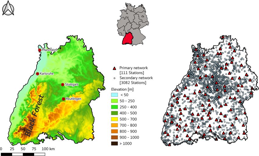
584             A. Bárdossy et al.: The use of personal weather station observations to improve precipitation estimation

   Against the backdrop of low precipitation station densi-       usually much lower. This paper is organized as follows: after
ties, the additional data from PWSs have a high potential to      the introduction, the methodology for finding useful infor-
improve the information of spatial and temporal precipita-        mation and the subsequent interpolation steps is described.
tion characteristics. However, one of the major drawbacks of      The described procedure was used for precipitation events of
PWSs precipitation data is their trustworthiness. There is lit-   the last 4 years in the federal state of Baden-Württemberg
tle systematic control on the placing and correct installation    in southwestern Germany. The results of the interpolation
and maintenance of the PWSs, so it is usually not known           and the corresponding quality of the method are discussed
whether a PWS is set up according to the international stan-      in Sect. 4. The paper ends with a discussion and conclusions.
dards published by the World Meteorological Organization
(WMO; World Meteorological Organization, 2008). Further-
more, there is no information available about the mainte-         2   Study area and data
nance of PWSs. Therefore, precipitation data from PWSs
may contain numerous errors resulting from incorrect instal-      The federal state of Baden-Württemberg is located in
lation, poor maintenance, faulty calibration and data transfer    southwestern Germany and has an area of approximately
errors (de Vos et al., 2017). This shows that the data from       36 000 km2 . The annual precipitation varies between 600 and
PWS networks cannot be regarded as being as reliable as           2100 mm (Deutscher Wetterdienst, 2020), and the highest
those of professional networks operated by national weather       amounts are recorded in the higher elevations of the moun-
services or environmental agencies. Consequently, the use of      tain ranges of the Black Forest. The rain gauge network of
PWS data requires specific efforts to detect these errors and     the German Weather Service (DWD) in Baden-Württemberg
take them into account.                                           (referred to as the primary network from here on) currently
   For air temperature measurements, Napoly et al. (2018)         comprises 111 stations for the study period, with high tem-
developed a quality control (QC) procedure to filter out sus-     poral resolution data (Fig. 1). The gauges used in this net-
picious measurements from PWS stations that are caused, for       work are predominantly weighing gauges. This precipitation
example, by solar exposition or incorrect placement. For pre-     data are available in different temporal resolutions from the
cipitation, de Vos et al. (2017) investigated the applicabil-     Climate Data Center of the DWD. For this study, hourly pre-
ity of personal stations for urban hydrology in Amsterdam,        cipitation data were used.
the Netherlands. They reported the results of a systematic           For the PWS data, the Netatmo network was selected
comparison of an official observation by the Royal Nether-        (https://weathermap.netatmo.com, last access: 3 Febru-
lands Meteorological Institute (KNMI) and three PWS Ne-           ary 2021). The stations from this PWS network (referred to
tatmo rain gauges. This provides information on the quality       as the secondary network from here on) show an uneven dis-
of the measurements in the case of the correct installation       tribution in space, which mainly reflects the population den-
of the devices. As many of the PWSs may be placed with-           sity and topography of the study area (Fig. 1). The number of
out consideration of the WMO standards, the results of these      secondary stations is higher in densely populated areas, such
comparisons cannot be transferred to the other PWS observa-       as in the Stuttgart metropolitan area and the Rhine–Neckar
tions. In a more recent study, de Vos et al. (2019) developed a   metropolitan region between Karlsruhe and Mannheim. Fur-
QC methodology of PWS precipitation measurements based            thermore, there are no secondary network stations above
on filters which detect faulty zeroes, high influxes and sta-     1000 m above sea level (a.s.l.); however, the primary network
tions outliers based on a comparison between neighbouring         only has one station above 1000 m (at the Feldberg sum-
stations. A subsequent bias correction is based on a compar-      mit at 1496 m) as well. The number of gauges from the sec-
ison of past observations with a combined rain gauge and          ondary network varies over time. The time period from 2015
radar product (de Vos et al., 2019).                              to 2019 was considered for this study as the number of avail-
   Overall, the data from PWS rain gauges may provide use-        able PWSs before 2015 was very low. At the end of this time
ful information for many precipitation events and may also        period, over 3000 stations from the secondary network were
be useful for real-time flood forecasting, but data quality is-   available. Figure 2 shows the number of secondary stations as
sues have to be overcome. In this paper, we focus on the          a function of time and the length of the time series. One can
use of PWS data for the interpolation of intense precipitation    see that many stations have less than 1 year of observations,
events. We propose a two-fold approach based on indicator         which is the reasonable length of a series for the suggested
correlations and spatial patterns to filter out suspicious mea-   method. Presently, it cannot accommodate series shorter than
surements and to use the information from PWSs indirectly.        1 year (excluding time periods with snowfall), but as the se-
Thus, the basic assumption is that many of the stations may       ries are becoming longer, more and more PWS observations
be biased but are correct in terms of the temporal order. For     become useful.
the spatial pattern, information from a reliable precipitation       The Netatmo rain gauges are plastic tipping buckets which
network, e.g. from a national weather service, is required.       have an opening orifice of 125 cm2 (compared to 200 cm2 for
These measurements are considered to be more trustworthy          the primary network). A detailed technical description of the
than the PWS data; however, the number of such stations is        Netatmo PWS is given by de Vos et al. (2019). Since these

Hydrol. Earth Syst. Sci., 25, 583–601, 2021                                        https://doi.org/10.5194/hess-25-583-2021

A. Bárdossy et al.: The use of personal weather station observations to improve precipitation estimation                        585

Figure 1. Map of the federal state of Baden-Württemberg, showing the topography and the location of the DWD (primary) and Netatmo
(secondary) gauges.

Figure 2. Development of the number of available online Netatmo rain gauges (a) and length of available valid hourly observations in
Baden-Württemberg (b).

devices are not heated, their usage is limited to liquid precipi-      In order to assess the spatial variability within a dense net-
tation. To take this into account, data from secondary stations     work of primary gauges, the precipitation data from the mu-
were only used in case the average daily air temperature at         nicipality of Reutlingen (located about 30 km south of the
the nearest DWD station was above 5 ◦ C. Data from the Ne-          state capital of Stuttgart) was additionally used. This city
tatmo PWS network can be downloaded from the Netatmo                has operated a dense network of 12 weighing rain gauges
API either as raw data with irregular time intervals or in dif-     (OTT Pluvio2 ) since 2014 in an area of 87 km2 (not shown
ferent temporal resolutions down to 5 min. Further informa-         in Fig. 1). Furthermore, three Netatmo rain gauges were in-
tion on how the raw data are processed to different temporal        stalled at the institute’s own weather station on the campus
aggregations is not available on the manufacturer’s website.        of the University of Stuttgart, where a Pluvio2 weighing rain
For this study, the hourly precipitation data from the Netatmo      gauge is installed as well. This allows a direct comparison
API was used.                                                       between the gauges from the primary network and the sec-

https://doi.org/10.5194/hess-25-583-2021                                            Hydrol. Earth Syst. Sci., 25, 583–601, 2021
586                A. Bárdossy et al.: The use of personal weather station observations to improve precipitation estimation

ondary network in cases where the latter are installed and                     In order to identify stations which are likely to deliver rea-
maintained correctly.                                                       sonable data for high intensities, indicator correlations are
                                                                            used. The distribution function of precipitation at location x
                                                                            is denoted as Fx,1t (z), and the one for secondary observa-
3     Methodology                                                           tions at locations yj is denoted as Gyj ,1t (z), respectively.
                                                                            For a selected probability α, the indicator series is as follows:
It is assumed that the secondary stations may have individ-
ual measurement problems (e.g. incorrect placement, lack of
                                                                                                1 if Fx,1t (U1t (x, t)) > α
and/or wrong maintenance and data transmission problems),                   Iα,1t,Z (x, t) =                                  .           (2)
                                                                                                0 else
and due to their large number, there is no possibility to di-
rectly check their proper placing and functioning. Further-                 For a secondary location yj , it is as follows:
more, at many locations (especially in urban areas) there is
no possibility to set up the rain gauges in such a way that they                              1 if Gyj ,1t Y1t yj , t > α
                                                                            Iα,1t,Y yj , t =                                 .            (3)
fulfil the WMO standards. Therefore, the goal is to filter out                                 0 else
stations which deliver data contradicting the observations of
the primary network which meet the WMO standards.                           Under the order assumptions of Eq. (1), for any sec-
   Observations from the primary and secondary network                      ondary location yj the two indicator series are identical
were used in hourly time steps and can be aggregated to dif-                Iα,1t,Z (yj , t) = Iα,1t,Y (yj , t). Thus, the spatial variability
ferent durations 1t. The usefulness of the secondary data is                in Iα,1t,Z and Iα,1t,Y has to be the same.
investigated for different temporal aggregations. Z1t (x, t) is                For any two locations corresponding to the primary net-
the (partly unknown) precipitation at location x and time t in-             work xi and xj and any α and 1t, the correlation (in time) of
tegrated over the time interval 1t. It is assumed that this pre-            the indicator series is ρZ,α,1t (xi , xj ) and provides informa-
cipitation is measured by the primary network at locations                  tion on how precipitation series vary in space. This indicator
{x1 , . . . , xN }. The measurements of the secondary network               correlation usually decreases with increasing separation dis-
are indicated by Y1t (yj , t) at locations {y1 , . . . , yM }. Note         tance. This decrease is not at the same rate everywhere and
that Y is not considered to be a spatially stationary random                is not the same for different thresholds and aggregations. For
field. The basic assumption for the suggested quality control               the secondary network, indicator correlations ρZ,Y,α,1t (xi ,
and bias correction method is that the measured precipita-                  yj ) with the series in the primary network can be calcu-
tion data from the secondary network may be biased in their                 lated. Following the hypothesis from Eq. (1), these correla-
values but correct in terms of their order – at least for high              tions should be similar and can be compared to the indicator
precipitation intensities. This means that at times t1 and t2               correlations calculated from pairs of the primary network.
the following inequality holds:                                                The sample size has a big influence on the variance in
                                                                            the indicator correlations. Therefore, to take into account the
Y1t (yi , t1 ) < Y1t (yi , t2 ) ⇒ Z1t (yi , t1 ) < Z1t (yi , t2 ) .   (1)   limited interval of availability of the secondary observations,
This means that the measured precipitation amount from the                  indicator correlations of the primary network, corresponding
secondary network is likely to have an unknown, location-                   to the same periods for which the secondary variable is avail-
specific bias, but the order of the values at a location is                 able, are used for the comparison. This is done individually
preserved. This assumption is reasonable, specifically for                  for each secondary site. A secondary station is flagged as sus-
high precipitation intensities, and supported by measure-                   picious if its indicator correlations with the nearest primary
ments presented in the results section.                                     network points are below the lowest indicator correlation cor-
   For QC, two filters are applied. The first one is an                     responding to the primary network for the same time steps
indicator-based filter (IBF) which compares the secondary                   and at the nearly same separation distance. A certain toler-
time series with the closest primary series and focuses on                  ance 1d for the selection of the pairs of the primary network
intense precipitation. The precipitation values of the remain-              is needed due to the irregular spacing of the secondary sta-
ing PWS stations are then bias corrected using quantile map-                tions and the natural variability in precipitation. This means
ping. The second filter is an event-based filter (EBF) de-                  that if, in the following:
signed to remove individual contradictory observations for
                                                                            ρZ,Y,α,1t xi , yj < min ρZ,α,1t (xk , xm ) ;
a given time step using a spatial comparison. These two fil-
ters and the bias correction are described in the following                             k (xk − xm ) − xi − yj k < 1d ,                    (4)
sections.
                                                                            then the secondary station shows a weaker association to the
3.1    High intensity indicator-based filtering (IBF)                       primary than what one would expect from primary observa-
                                                                            tions. In this case, it is reasonable to discard the measured
As a first step in quality control, all PWSs with notoriously               time series corresponding to the secondary network at loca-
inconsistent rainfall values are removed. For this purpose, the             tion yi . This procedure can be repeated for a set of selected
dependence between neighbouring stations is investigated.                   α values.

Hydrol. Earth Syst. Sci., 25, 583–601, 2021                                                    https://doi.org/10.5194/hess-25-583-2021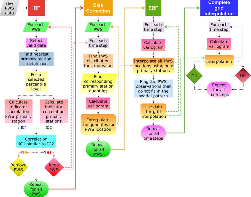
A. Bárdossy et al.: The use of personal weather station observations to improve precipitation estimation                        587

   Under the assumption that the temporal order of the pre-         location yj , the observed percentile of precipitation is as fol-
cipitation at secondary locations is correct (Eq. 1), one could     lows:
have used rank correlations instead of the indicator correla-
tions. The indicator approach is preferred, however, as the         P1t yj , t = Gyj ,1t Y1t yj , t .                             (5)
sensitivity of the devices of the primary and secondary net-
works is different, and this would influence the order of the       For the observations of the primary network, the quantiles of
small values strongly. Furthermore, random measurement er-          the precipitation distribution at the primary stations are se-
rors would also influence the order of low values. In order to      lected. The distributions at the primary stations are based on
have a sufficient sample size and to have robust results, high      the same time steps as those which have valid observations at
α values and low temporal aggregations 1t are preferred.            the target secondary station. In this way, a possible bias due
                                                                    to the short observation period at the secondary location can
3.2   Bias correction – precipitation amount estimation             be avoided. The quantiles are as follows:
      for secondary observations                                                  −1
                                                                    Q1t (xi ) = F1t,x i
                                                                                        P1t yj , t .                            (6)
After the selection of the potentially useful secondary sta-        These quantiles are interpolated using OK to obtain an esti-
tions, the next step is to correct their observations. The as-      mate of the precipitation at the target location.
sumption in Eq. (1) means that the measured precipitation
amounts from the secondary network are likely to have an                       Xn
                                                                     o
unknown bias, but the order of the values at a location is pre-     Z1t yj , t =   λi Q1t (xi ) .                                (7)
served. This assumption is likely to be reasonable for high                        i=1
precipitation intensities. Thus, the percentile of the precipi-     Here, the λi − s are the weights calculated using the Kriging
tation observed at a given time at a secondary location can         equations. Note that the precipitation amount at the target lo-
be used for the estimation of the true precipitation amounts.       cation is obtained via interpolation, but the interpolation is
Since this is a percentile and not a precipitation amount, it       not done by using the primary observations corresponding to
has to be converted to a precipitation amount for further use.      the same time but by using the quantiles corresponding to the
This can be done using the distribution function of precipita-      percentile of the target secondary station observation. Thus,
tion amounts corresponding to the location yj and the aggre-        these values may exceed all values observed at the primary
gation 1t. As the observations from the secondary network           stations at time t. Note that this correction of the secondary
could be biased, their distribution Gyj ,1t cannot be used for      observations is non-linear. This procedure is used for all loca-
this purpose. Thus, one needs an unbiased estimation of the         tions which were accepted after application of the indicator
local distribution functions.                                       filter. In this way, the bias from observed precipitation val-
   Distribution functions based on long observation series are      ues at the secondary stations is removed using the observed
available for the locations of the primary network. For loca-       percentiles and the distributions at the primary stations. This
tions of the secondary network, they have to be estimated           transformation does not require an independent ground truth
via interpolation. This can be done by using different geo-         of best estimation of precipitation at the secondary locations.
statistical methods. A method for interpolating distribution
functions for short aggregation times is presented in Mosthaf       3.3   Event-based spatial filtering (EBF)
and Bárdossy (2017). Another possibility is to interpolate the
quantiles corresponding to selected percentiles or interpolat-      While some stations may work properly in general, due to
ing percentiles for selected precipitation amounts. Another         unforeseen events (such as battery failure or transmission
option for estimating distribution functions corresponding to       errors) they may deliver individual faulty values at certain
arbitrary locations is to use functional Kriging (Giraldo et al.,   times. In order to filter out these errors, a simple geostatis-
2011) to interpolate the distribution functions directly. The       tical outlier detection method is used, as described in Bár-
advantage of interpolating distribution functions is that they      dossy and Kundzewicz (1990). The geostatistical methods
are strongly related to the geographical locations of the se-       used for outlier detection and the interpolation of rainfall
lected location and also to topography. These variables are         amounts require the knowledge of the corresponding vari-
available in a high spatial resolution for the whole investiga-     ogram. However, the highly skewed distribution of the pre-
tion domain. Additionally, observations from different time         cipitation amounts makes the estimation of the variogram
periods and temporal aggregations can also be taken into ac-        difficult. Instead, one can use rank-based methods for this
count as co-variates.                                               purpose, as suggested in Lebrenz and Bárdossy (2017), and
   In this paper, ordinary Kriging (OK) is used for the inter-      rescale the rank-based variogram.
polation of the quantiles and for the percentiles to construct         For a given temporal aggregation 1t, time t and target sec-
the distribution functions for both the locations of the sec-       ondary location yj , the precipitation amount is estimated via
ondary observations and for the whole interpolation grid. For       OK using the observations of aggregation 1t at time t of
a given temporal aggregation 1t, time t and target secondary        primary stations. This value is denoted as Z1t  ∗ (y , t). If the
                                                                                                                        j

https://doi.org/10.5194/hess-25-583-2021                                            Hydrol. Earth Syst. Sci., 25, 583–601, 2021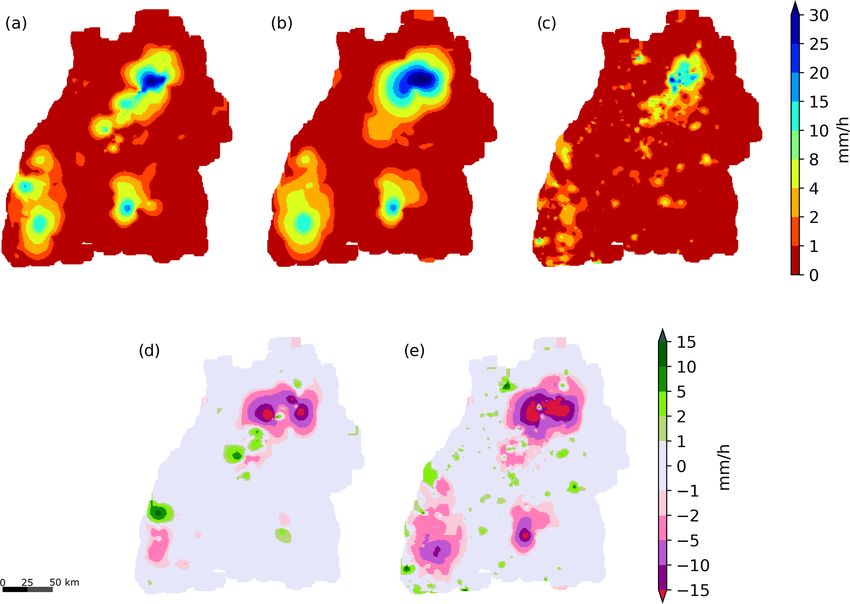
588              A. Bárdossy et al.: The use of personal weather station observations to improve precipitation estimation

precipitation amount at the secondary station estimated us-            The interpolation is based on the following observations:
ing Eq. (7) differs very much from Z1t∗ (y , t), the secondary
                                           j
location is discarded for the interpolation. As a limit for the     {u1 , . . ., uN } = {x1 , . . ., xN } ∪ {y1 , . . ., yM } .   (12)
difference, three times the Kriging standard deviation was
selected. Formally, in the following:                                  For any location x, we calculate as follows:
                                                                                      n
  ∗ y , t − Zo y , t
                                                                                    X
 Z1t                                                                 ∗
     j       1t j                                                   Z1t (x, t) =            λi (Z (ui , t) + ε (ui , t)) .        (13)
                      > 3.                                  (8)
     σ1t yj , t                                                                       i=1

                                                                      To minimize the estimation variance, an equation system
   This means that if the estimated precipitation at the sec-
                                                                    similar to the OK system has to be solved as in the following:
ondary location does not fit into the pattern of the primary
observations then it is discarded. Note that this filter is not     n
                                                                    X                         h          i
                                                                           λj γ ui − uj + λi E ε(ui , t)2 + µ = γ (ui − x)

necessarily discarding secondary observations which differ
from the primary ones – it only removes those for which             j =1
there is a strong local disagreement. This procedure is pre-                            n
                                                                                        X
dominantly removing false zeros at secondary observations           i = 1, . . ., n            λj = 1.                            (14)
which are, for example, due to a temporary loss in connec-                              j =1
tion between the rain gauge module and the Netatmo base
station.                                                               Note that OK is a special case of this procedure, with the
                                                                    additional assumption ε(yj , t) = 0. This system leads to an
3.4   Interpolation of precipitation amounts                        increase in the weights for the primary network and a de-
                                                                    crease in the weights for the secondary network. For each
After the application of the two filters and the bias correction,   time step and percentile, the variances in the random error
the remaining PWS data can be used for spatial interpola-           terms ε(yi , t) are estimated from the interpolation error of
tion. Once the percentiles of the secondary locations are con-      the distribution functions. This interpolation method is re-
verted to precipitation amounts, different Kriging procedures       ferred to as Kriging using uncertain data (KU) (Delhomme,
can be used for the interpolation over a grid in the target re-     1978). The variograms used for interpolation were calculated
gion. The simplest solution is to use OK. For aggregations of       in the rank space using the observations of the primary net-
1 d or longer, the orographic influence should be taken into        work only, which leads to more robust results (Lebrenz and
account. This can be done by using external drift Kriging           Bárdossy, 2017). Anisotropy was not considered; the main
(Ahmed and de Marsily, 1987).                                       reason for this was that the primary network did not give ro-
   A problem that remains when using these Kriging proce-           bust results.
dures is that the precipitation amounts of the secondary net-
work are more uncertain than those of the primary network.          3.5     Step-by-step summary of the methodology
To reflect this difference, a modified version of Kriging, as
described in Delhomme (1978), is applied. This allows for a         Figure 3 shows a flow chart of the procedure for obtaining
reduction in the weights for the secondary stations.                interpolated precipitation grids from raw PWS data. In sum-
   Suppose that, for each point yi time t and temporal aggre-       mary, the procedure for using secondary observations is as
gation 1t, there is an unknown error of the percentiles ε(yi ,      follows:
t) which has the following properties:                                1. Select a percentile threshold for a selected temporal ag-
  1. unbiased, i.e.                                                      gregation. The threshold should be adapted to the tem-
                                                                         poral aggregation, e.g. 98 % or 99 % for 1 h or 95 % for
                                                                         3 h data.

     E ε (yi , t) = 0;                                       (9)
                                                                      2. Calculate the indicator series for primary and secondary
  2. uncorrelated, i.e.                                                  stations corresponding to the percentile threshold.

     E ε (yi , t) ε yj , t = 0 if i 6 = j ;                 (10)      3. Implement the following procedure for each individual
                                                                         secondary station:
  3. uncorrelated with the parameter value, i.e.
                                                                             a. calculate the indicator correlation of the given sec-
                                                                                ondary and the closest primary station;

     E ε (yi , t) Z (yi , t) = 0.                           (11)
                                                                             b. calculate the indicator correlations of all primary
  For the primary network, we assume that ε(xi , t) = 0.                        stations using data corresponding to the time steps
                                                                                of the selected secondary station;

Hydrol. Earth Syst. Sci., 25, 583–601, 2021                                                  https://doi.org/10.5194/hess-25-583-2021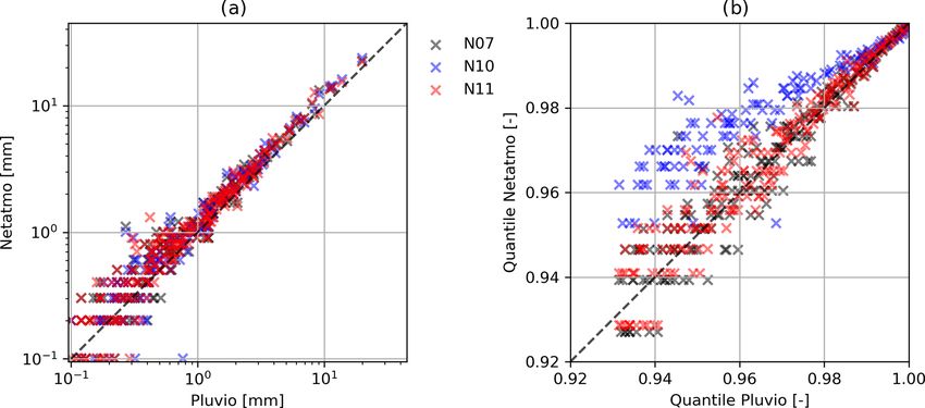
A. Bárdossy et al.: The use of personal weather station observations to improve precipitation estimation                             589

Figure 3. Flow chart illustrating the procedure from raw PWS data to interpolated precipitation grids.

       c. compare the correlations and keep the secondary                   6. Interpolate precipitation for each secondary location us-
          station if its indicator correlation is in the same                  ing OK, excluding the value assigned to the location
          range as the indicator correlations of the primary                   (cross validation mode).
          stations approximately at the same distance (i.e.
                                                                            7. Compare the interpolated and the assigned value from
          IBF).
                                                                               step 5.c and remove station if condition of inequality
  4. Perform a bias correction by interpolating the distribu-                  (Eq. 8) indicates outlier.
     tion function values of the primary network.
                                                                            8. Interpolate precipitation for a target grid using all re-
  5. Select an event to be interpolated, and calculate the cor-                maining values.
     responding variogram of precipitation (based on rank
     statistics).                                                       4     Application and results
       a. Calculate the percentile of observed precipitation
                                                                        The section describing the application of the methodology is
          (based on the corresponding time series).
                                                                        divided into three parts. First, the rationale of the assump-
       b. Calculate the quantiles corresponding to the above            tions is investigated. In a second step, the methodology is
          secondary percentile for the closest M primary sta-           applied on a large number of intense precipitation events on
          tions of observed precipitation (based on the corre-          different temporal aggregations using a cross validation ap-
          sponding time series).                                        proach. This allows for an objective judgement of the appli-
       c. Interpolate the quantiles for the location of the sec-        cability of the results. Finally, the results of the interpolation
          ondary station using the above primary values, us-            on a regular grid are shown and compared.
          ing OK, and assign the obtained value to the sec-
          ondary location.                                              4.1    Justification of the methods

                                                                        For a direct comparison between the secondary rain gauges
                                                                        and devices from the primary network, three Netatmo rain

https://doi.org/10.5194/hess-25-583-2021                                                 Hydrol. Earth Syst. Sci., 25, 583–601, 2021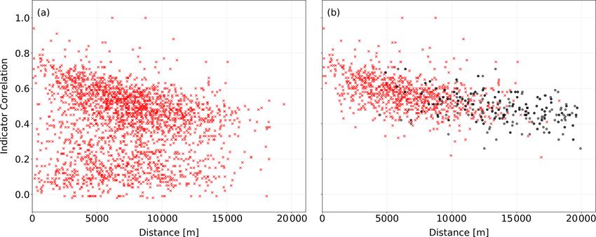
590             A. Bárdossy et al.: The use of personal weather station observations to improve precipitation estimation

gauges were installed next to a Pluvio2 weighing rain gauge         tile, using pairs of observations from the primary–primary
(the same type as regularly used by the DWD) at the weather         and the primary and secondary network as a function of sta-
station of the Institute for Modelling Hydraulic and Environ-       tion distance. The indicator correlations of the pairs of the
mental Systems (IWS) on the campus of the University of             primary network show relatively high values and a slow de-
Stuttgart. With this data from 15 May to 15 October 2019, a         crease with increasing distance. In contrast, if the indicator
direct comparison between the different devices used in the         correlations are calculated using pairs with one location cor-
primary and secondary network was possible.                         responding to the primary network and one to the secondary
   Table 1 shows statistics of the three devices compared to        network, the scatter increased substantially. Secondary sta-
those of the reference station. The secondary stations overes-      tions for which the indicator correlations are very small in
timated precipitation amounts by about 20 %. It can be ob-          the sense of Eq. (4) are considered as unreliable and are re-
served that the differences between the reference and the           moved from further processing. A relatively large distance
Netatmo gauge are not linear; hence, a data correction of           tolerance was used, as the density of the primary stations
the secondary gauges, using a linear scaling factor, is not         is much lower than the density of the secondary stations.
sufficient. Furthermore, the maximum in the sub-daily ag-           In Fig. 6, the indicator correlations corresponding to the re-
gregations from N10 shows an outlier. This was caused by            maining secondary stations show a similar spatial behaviour
an interrupted connection between the rain sensor and the           as the primary network. In our case, 2462 of the originally
base station. In this case, the total sum of the precipitation      available 3082 stations remained, with a time series length
over a longer time period was transferred at once (i.e. in one      of more than 2 months. After applying the IBF filter, a set
single measurement interval) when the connection was re-            of 862 (35 %) PWSs remained. This is a relatively small frac-
established. Such transmission errors lead to outliers which        tion of the total number of secondary stations, but note that
falsify the results. Figure 4 shows scatter plots of hourly rain-   the shortest records were removed, and low correlations may
fall data and the corresponding percentiles from these three        occur as a consequence of the short observation periods. In
Netatmo gauges and the reference station. The occurrence of         the future, with an increasing number of measurements, some
high values and percentiles is similar for the primary and the      of these stations may be reconsidered.
secondary devices. The Netatmo station N10, however, devi-             The effect of the IBF was checked by calculating the rank
ates substantially from the other measurements in the quan-         correlations between pairs of primary and PWS stations with
tile plot (Fig. 4b), which also points to data transmission er-     a distance below 2500 m. Figure 7 shows that the removed
rors in which the station failed to transmit data during rain       PWSs have a low rank correlation to their primary neigh-
events. The indicator-filtering procedure (i.e. IBF) can iden-      bours, while, for the accepted ones, the majority of the rank
tify such problems effectively.                                     correlations is high. These high rank correlations support the
   The secondary measurement devices can also have very             rank-based hypothesis formulated in Eq. (1).
different biases, depending on where and how they are in-              The EBF was applied for each event individually. The
stalled. This can be seen by comparing the distribution func-       number of discarded secondary stations is this study varied
tions of hourly precipitation data from nearby primary and          from event to event and was on average around 5 %.
secondary stations in the same area. Figure 5 shows the em-
pirical distribution functions of three primary and four sec-       4.3   Bias correction
ondary stations in the city of Reutlingen. While the distri-
bution functions of the primary network are nearly identi-          The bias correction method is illustrated using the example
cal, those of the nearest secondary stations vary strongly.         shown in Fig. 8. For simplicity, the four primary stations in
Some overestimate and others underestimate the amounts              the corners of a square and the secondary station in the centre
significantly. This example supports the concept of the pa-         of this square are considered. This configuration ensures that
per, namely that secondary data require filtering and data          the OK weights of the primary station with respect to the sec-
transformations before use. While the distributions differ,         ondary station are all equal to one-quarter, independent of the
the probability of no precipitation p0 (defined as precipita-       variogram. The observed precipitation amounts at the corner
tion < 0.1 mm) ranges from 0.90 to 0.91 and is thus very            stations are 3.1, 1.8, 3.0 and 2.1 mm for a selected event. The
similar for both types of stations, indicating that the occur-      secondary station in the centre recorded 1.7 mm of rainfall.
rence of precipitation can be well detected by the secondary        This corresponds to the 0.99 non-exceedance probability of
network.                                                            precipitation for the specific secondary station. The precipi-
                                                                    tation quantiles at the primary stations corresponding to the
4.2   Application of the filters                                    0.99 probability are 3.2, 3.5, 3.1 and 3.0 mm. Interpolation of
                                                                    these values gives 3.2 mm, which is the value assigned to the
Indicator correlations were calculated for different temporal       secondary station instead of the value of 1.7 mm. This value
aggregations and for a large number of different α values in        is greater than all the four primary observations. The rea-
the range between 95 % and 99 %. Figure 6 shows the in-             son for this is that the primary observations all correspond to
dicator correlations for 1 h aggregation and the 99 % quan-         lower percentiles. Note that the interpolation of the primary

Hydrol. Earth Syst. Sci., 25, 583–601, 2021                                           https://doi.org/10.5194/hess-25-583-2021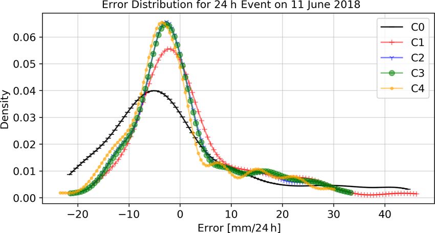
A. Bárdossy et al.: The use of personal weather station observations to improve precipitation estimation                                                               591

Table 1. Statistics of three Netatmo stations (N07, N10 and N11) compared to a Pluvio2 weighing gauge for April to October 2019 at the
IWS meteorological station for different temporal aggregations.

                                                            1h                                                   6h                                     24 h
                                       Pluvio2         N07         N10        N11            Pluvio2         N07         N10        N11    Pluvio2    N07       N10     N11
  p0 (–)                                   0.92       0.84        0.94        0.91              0.82        0.75        0.84        0.82     0.59     0.56      0.65    0.59
  Mean (mm)                                1.24       1.46        1.80        1.41              3.46        4.04        4.24        3.89     5.78     7.28      7.51    7.02
  Standard deviation (mm)                  2.15       2.52        4.49        2.52              4.86        5.77        7.55        5.71     8.46    10.49     11.52   10.33
  25th percentile (mm)                     0.18       0.20        0.10        0.20              0.39        0.33        0.30        0.40     0.48     0.63      0.58    0.58
  50th percentile (mm)                     0.51       0.71        0.50        0.61              1.49        1.41        0.91        1.21     2.36     2.78      1.62    2.58
  75th percentile (mm)                     1.34       1.72        1.41        1.52              4.60        5.33        4.14        4.95     7.82     9.87     11.26    9.95
  Maximum (mm)                            19.84      22.62       44.74       22.22             23.28       28.58       44.74       27.98    45.62    55.55     56.16   55.55
All statistics, except for the p0 values, are based on non-zero values. p0 is the non-exceedance probability of precipitation < 0.1 mm.

Figure 4. Scatter plot showing (a) the hourly rainfall values (axes log scaled) and (b) the corresponding upper percentiles > 0.92 (b) between
the Pluvio2 weighing gauge and three Netatmo gauges (N07, N10 and N11) at the IWS meteorological station.

values corresponding to the event for the secondary observa-                                         The cross validation was carried out for a set of different
tion location would be 2.5 mm.                                                                    temporal aggregations 1t and a set of selected events. Only
   The bias in the PWS observations can be recognized by in-                                      times with intense precipitation were selected. Table 2 shows
vestigating data with a higher temporal aggregation. A com-                                       some characteristics of the selected events. For short time pe-
parison of monthly or seasonal precipitation amounts at pri-                                      riods, nearly all events were from the summer season, while
mary stations and PWSs reveals whether there is a systematic                                      for higher aggregation the number of winter season events
difference or not. As monthly or seasonal precipitation can                                       increased, but their portion remained below 30 %.
be well interpolated by using primary stations only (temporal                                        The improvement obtained through the use of secondary
aggregation increases the quality of interpolation; Bárdossy                                      data is demonstrated using a cross validation procedure. The
and Pegram, 2013), this comparison provides a good indica-                                        primary network is randomly split into 10 subsets of 10 or
tion of bias. The difference between the interpolated and the                                     11 stations each. The data of each of these subsets were
PWS aggregations is different from PWS to PWS and often                                           removed and subsequently interpolated using two different
exceeds 20 %. Both positive and negative deviations occur.                                        configurations of the data used, namely (a) only other pri-
This points out that bias correction has to be done for each                                      mary network stations and (b) using the other primary and
station separately.                                                                               the secondary network stations. For the latter case, the inter-
                                                                                                  polations were carried out using the primary station data and
4.4     Cross validation results                                                                  the following configurations:
As there is no ground truth available, the quality of the proce-
dure had to be tested by comparing omitted observations and
their estimates obtained after the application of the method.

https://doi.org/10.5194/hess-25-583-2021                                                                                 Hydrol. Earth Syst. Sci., 25, 583–601, 2021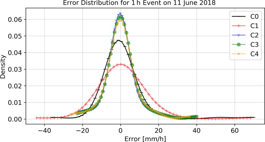
592              A. Bárdossy et al.: The use of personal weather station observations to improve precipitation estimation

Figure 5. Probability of no precipitation (a) and the upper part of the empirical distribution functions (b) for three primary stations (solid
lines) and four secondary stations (dashed lines) from a small area in the city of Reutlingen, based on a sample size of 15 990 data pairs
(hourly precipitation). The distance between the primary stations is between 5.5 and 9 km, and the distances from the secondary stations to
the next primary stations range from 1 to 3 km.

Figure 6. Indicator correlations for 1 h temporal resolution and α = 0.99 between the secondary network and the nearest primary network
stations before (a) and after (b), applying the IBF (red crosses). The black dots refer to the indicator correlation between the primary network
stations.

  – C1 – all secondary stations;                                             First, the measured and interpolated values were compared
                                                                          for each individual station, and the Pearson (r) and Spearman
  – C2 – secondary stations remaining after the application               correlations (rS ) of the observed and interpolated series were
    of the IBF;                                                           calculated. Table 3 shows the results for the different config-
  – C3 – secondary stations remaining after application of                urations used for the interpolation.
    the IBF and the EBF;                                                     There is no improvement if no filter is applied – except for
                                                                          a very slight improvement for 1 h durations. This is mainly
  – C4 – secondary stations remaining after application of                due to the better identification of the wet and dry areas. The
    the IBF and the EBF and considering uncertainty (KU).                 use of the filters (and the subsequent transformation of the
                                                                          precipitation values) leads to an improvement in the estima-
   The results were compared to the observations of the re-               tion, with the IBF being the most important. The spatial filter
moved stations. The comparison was done for each location                 further improves the correlation, while the additional con-
using all time steps and at each time step using all locations.           sideration of the uncertainty of the corrected values at the
Different measures, including those introduced in Bárdossy                secondary network results in a marginal improvement for the
and Pegram (2013), were used to compare the different in-                 selected events. As the secondary stations are not uniformly
terpolations. The results were evaluated for each temporal                distributed over the investigated domain, the gain from us-
aggregation.

Hydrol. Earth Syst. Sci., 25, 583–601, 2021                                                   https://doi.org/10.5194/hess-25-583-2021
A. Bárdossy et al.: The use of personal weather station observations to improve precipitation estimation 593
Table 2. Statistics of the selected intense precipitation events based on the primary network.
Temporal resolution 1h 3h 6h 12 h 24 h
Number of intense events 185 190 190 195 195
Events between October–March 1 16 29 48 57
Events between April–September 184 174 161 147 138
Minimum of the maxim (mm) 28.01 31.2 33.35 34.9 35.5
Maximum of the maxima (mm) 122.3 158.2 158.4 160 210.3
p0 (mean of all stations and events) 0.9 0.84 0.77 0.68 0.55
p0 is defined here as precipitation < 0.1 mm.
Table 3. Percentage of the stations with improved temporal correlation (compared to interpolation using primary stations only) for the
configurations C1–C4.
Temporal aggregation 1h 3h 6h 12 h 24 h
Number of events 185 190 190 195 195
Correlation measure r rS r rS r rS r rS r rS
C1 – primary and all secondary, without filter and OK 60 68 40 57 31 49 22 34 17 32
C2 – primary and secondary, using IBF and OK 81 91 75 90 73 90 64 84 52 81
C3 – primary and secondary, using IBF, EBF and OK 81 92 75 93 73 92 69 92 56 87
C4 – primary and secondary, using IBF, EBF and KU 81 92 75 92 74 91 70 91 56 86
r – Pearson correlation; rS – Spearman correlation.
Figure 8. Example of transformation and bias correction of precip-
Figure 7. Histograms of the rank correlations between primary sta- itation amounts at a secondary station.
tions and PWSs for pairs with a distance less than 2500 m. Panel (a)
shows the rank correlations for the stations removed by the filter,
and panel (b) shows those which were accepted.
case. The reason for this is that the spatial pattern is reason-
ably well captured by the secondary network. With increas-
ing temporal aggregation, the improvement disappears as the
ing them is also not uniform. The highest improvements
role of the bias increases due to the decreasing number of
were achieved in and near urban areas with a high density
data, which can be used for bias correction. As in the case of
of secondary stations; a lesser improvement was achieved in
the temporal evaluation, the IBF (and the subsequent trans-
forested areas with few secondary stations.
formation of the precipitation values) leads to the highest im-
The measured and interpolated results were also compared
provement. The EBF plays a marginal role, and the consid-
for each event in space, and the correlations between the ob-
eration of the uncertainty leads to a slight reduction in the
served and the interpolated spatial patterns were calculated as
quality of the spatial pattern. The improvement is smaller for
well. Table 4 shows the frequency of improvements for the
higher temporal aggregations. Kriging with uncertainty did
different configurations, C1 to C4, used for the interpolation.
not improve the results.
The use of secondary stations leads to a frequent im-
provement in the spatial interpolation, even in the unfiltered
https://doi.org/10.5194/hess-25-583-2021 Hydrol. Earth Syst. Sci., 25, 583–601, 2021594 A. Bárdossy et al.: The use of personal weather station observations to improve precipitation estimation
Table 4. Percentage of the stations with improved spatial correlation (compared to interpolation using primary stations only) for the config-
urations C1–C4 (r – Pearson correlation; rS – Spearman correlation).
Temporal aggregation 1h 3h 6h 12 h 24 h
Number of events 185 190 190 195 195
Correlation measure r rS r rS r rS r rS r rS
C1 – primary and all secondary, without filter and OK 83 68 72 52 63 49 53 49 49 46
C2 – primary and secondary, using IBF and OK 96 97 90 93 90 93 84 89 80 85
C3 – primary and secondary, using IBF, EBF and OK 96 97 92 94 93 94 89 92 84 89
C4 – primary and secondary, using IBF, EBF and KU 93 94 90 92 90 93 84 89 80 87
Finally, all results were compared in both space and time. (precipitation measured at PWSs) for the application of co-
Here the root mean squared error (RMSE) was calculated for Kriging may not be appropriate for this combination of vari-
all events and control stations. Table 5 shows the results for ables. Considering the ranks of the secondary observations
the different configurations used for the interpolation. or other transformed values as co-variables may improve the
The improvement using the filters is high for each aggre- co-Kriging results, but this is not the primary topic of this
gation. The IBF is important for improving the interpolation paper.
quality. The EBF and the consideration of the uncertainty
of the secondary stations are of minor importance. The im- 4.5 Selected events
provement is the largest for the shortest aggregation (1 h),
where the RMSE decreased by 20 %, and the smallest for the As the cross validation results were showing improvements,
24 h aggregation, with an improvement of 4 %. This deterio- the data transformations and subsequent interpolations were
ration is caused by the decreasing spatial variability in pre- carried out for all selected events. As an illustration, four se-
cipitation at higher temporal aggregations. The processes that lected events are shown and discussed here.
lead to long-lasting precipitation are predominantly accom- The first example (Fig. 9) shows the results of the interpo-
panied by a more even distribution in precipitation in space lation of a 1 h aggregated precipitation amount for the time
and time. The use of KU for interpolation resulted only in a period from 15:00 to 16:00 LT on 11 June 2018. For this
minor improvement. Nevertheless, it is reasonable to assign event, 531 out of 862 PWSs had valid data (i.e. no miss-
lower weights to the less reliable PWS data. In order to check ing values) from which 476 remained after the EBF. Fig-
whether the selection of the events led to this result, a cross ure. 9a–c show three different precipitation interpolations for
validation for all 1 h time steps during the period from April this event, as follows:
to October 2019 (5136 time steps) was carried out. The re- a. using the combination of the two station networks after
sults are shown in Table 6. In this case, OK with secondary application of the filters and transformation of the sec-
data did not lead to an improvement. This is mainly caused ondary data;
by the irregular spatial distribution of the PWSs. Stations lo-
cated very close to each other can cause instabilities in the so- b. using the primary network only;
lution of the Kriging equations, leading to high positive and c. using all raw unfiltered and uncorrected data from the
negative weights. Introducing a small random error (1 %) to secondary network only.
the PWSs stabilizes the solution and leads to an improvement
in the interpolation. The more realistic random error of 10 % In Fig. 9, panel (d) shows the difference between (a)
further improves the results. and (b), and panel (e) shows the difference between (c)
Note that the use of the filtered and bias-corrected sec- and (b). The three panels from (a) to (c) are similar in their
ondary stations improves the interpolation quality even for rough structure, but there are important differences in the de-
other interpolation methods. Table 7 shows the results for tails. The interpolation using the primary network leads to a
the 185 events with 1 h aggregation. One can observe that relatively smooth surface. The unfiltered secondary-station-
KU gives the best results, but the simple interpolations of based interpolation is highly variable and shows distinct pat-
nearest neighbour or inverse distance also lead to better re- terns such as small dry and wet areas. The combination af-
sults than using primary stations only. The poor performance ter filtering and transformation is more detailed than the pri-
of the co-Kriging is surprising. For this study, we used the mary interpolation, and in some regions, these differences are
observations from the secondary stations as co-variables. The high. The map of the difference between the primary and the
linear relationship which is supposed to exist between the in- secondary-station-based interpolation (Fig. 9e) shows large
vestigated variable (precipitation) and the secondary variable regions of underestimation and overestimation by the sec-
ondary network. The differences between the primary and
Hydrol. Earth Syst. Sci., 25, 583–601, 2021 https://doi.org/10.5194/hess-25-583-2021A. Bárdossy et al.: The use of personal weather station observations to improve precipitation estimation 595
Table 5. RMSE (mm) for all stations and events.
Temporal aggregation 1h 3h 6h 12 h 24 h
Number of events 185 190 190 195 195
C0 – primary stations only and OK (reference) 5.97 6.97 7.34 7.71 8.35
C1 – primary and all secondary, without filter and OK 6.21 44.79 18.43 10.01 24.16
C2 – primary and secondary, using IBF and OK 4.83 6.05 6.61 7.33 8.29
C3 – primary and secondary, using IBF, EBF and OK 4.84 6.07 6.58 7.19 8.12
C4 – primary and secondary, using IBF, EBF and KU 4.82 6.02 6.53 7.15 8.08
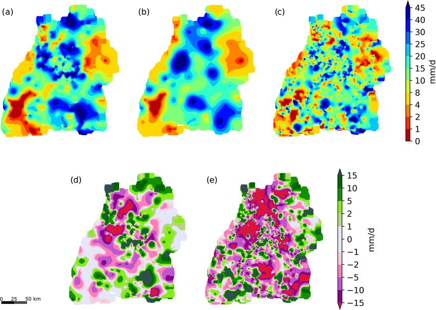
Figure 9. Interpolated precipitation for the time period from 15:00 to 16:00 LT on 11 June 2018 (a–c) and the differences between primary and
combination and primary and secondary data-based interpolations. Panel (a) shows the result after applying the filtering, (b) the interpolation
from the primary network and (c) the one from the secondary network. Panels (d) and (e) depict the differences between (a) and (b) and (c)
and (b), respectively.
Table 6. RMSE (in millimetres) and correlations for all stations Table 7. Bias and RMSE (in millimetres) for all stations and events
for all time steps (5136) between April and October 2019 for OK for different interpolation methods for 1 h aggregation.
and KU, with different error assumptions for 1 h aggregation.
Interpolation method Bias RMSE
Interpolation method RMSE Correlation Rank
correlation Ordinary Kriging; primary data only 0.05 5.97
Kriging with uncertainty; primary and PWSs 0.50 4.82
Primary stations OK 0.331 0.640 0.443
Primary and PWS OK 3.862 0.644 0.402
Nearest neighbour; primary and PWSs 0.89 5.06
Primary and PWS EK (1 % error) 0.314 0.759 0.578 Inverse distance; primary and PWSs 0.89 5.27
Primary and PWS EK (10 % error) 0.158 0.809 0.631 Co-Kriging; primary and PWSs 0.16 5.32
the filtered interpolations, using transformed secondary data of r from 0.36 to 0.77, of rS from 0.55 to 0.76 and a reduction
in panel (d), is much smaller, but in some regions, the dif- in the RMSE from 12.5 to 8.2 mm.
ferences are still quite large, e.g. in the northeastern part Figure 10 shows the distributions of the cross validation
of the study area. In both cases, negative and positive dif- errors for the different interpolations for this event. This is
ferences occur. Note that, for this data, the cross validation a typical case in which all methods yield unbiased results.
based on the primary observations showed an improvement The use of unfiltered and uncorrected secondary observa-
https://doi.org/10.5194/hess-25-583-2021 Hydrol. Earth Syst. Sci., 25, 583–601, 2021596 A. Bárdossy et al.: The use of personal weather station observations to improve precipitation estimation
the 1 h aggregations. This is caused by the reduction in the
variability with an increasing number of observations. Note
that, for this event, the cross validation based on the primary
observations showed an improvement of r from 0.57 to 0.8,
of rS from 0.57 to 0.82 and a reduction in the RMSE from
15.99 to 13.61 mm.
Another interesting 24 h event which was recorded on
28 July 2019 is shown in Fig. 13. For this event, 734 valid
PWSs remained from IBF and 703 after EBF. The map based
on the raw secondary data in Fig. 13c shows very scattered
intense rainfall. The combination of the primary and sec-
ondary observations changes the structure and the connec-
Figure 10. Distribution of the cross validation errors for the time
tivity of these area with intense precipitation. The cross vali-
period from 15:00 to 16:00 LT on 11 June 2018 for the five inter-
polation methods. C0 – using primary stations only and OK; C1 dation for this event showed an improvement of r from 0.32
– primary and all secondary, without filter and OK; C2 – primary to 0.75, of rS from 0.42 to 0.77 and a reduction in the RMSE
and secondary, using IBF and OK; C3 – primary and secondary, us- from 14.77 to 10.21 mm.
ing IBF, EBF and OK; C4 – primary and secondary, using IBF, EBF The results of the filtering algorithm for the other events
and KU. show a similar behaviour. The differences between primary
and combined interpolation can be both positive and nega-
tive for all temporal aggregations. In general, the secondary
tions (C1) shows the highest variance, followed by the in- network provides more spatial details, which could be very
terpolation using only primary observations (C0). The other important for the hydrological modelling of mesoscale catch-
three methods (C2–C4) have very similar results with signif- ments.
icantly lower variance. Figure 14 shows the distributions in the cross validation
Another interpolated 1 h accumulation corresponding to errors for the different interpolations for this event. The re-
17:00 to 18:00 LT on 6 September 2018 is shown in Fig. 11. sults are different from the case presented in Fig. 10. In this
For this event, from the 862 PWSs remaining after the IBF, case, all methods are slightly biased. The interpolation using
576 PWSs had available data, from which 513 remained af- only primary observations (C0) shows the highest bias and
ter the EBF. These pictures show a similar behaviour to those variance. In this case, the use of unfiltered and uncorrected
obtained for 11 June 2018 (Fig. 9). Here, a high local rain- secondary observations (C1) yields a lower bias and a lower
fall in the southern central part of the study area was obvi- variance. The other three methods (C2–C4) have very similar
ously not captured by the secondary network, leading to a results with significantly lower variance.
large local underestimation in Fig. 9e. Furthermore, a larger
area with precipitation in the primary network in the northern
central region in Fig. 9b is significantly reduced in size by the 5 Discussion
rainfall/no-rainfall information from the secondary network
in Fig. 9c. For this case, the cross validation based on the pri- The use of observations from such PWS networks has the
mary observations showed an improvement of r from 0.61 potential to improve the quality of precipitation estimations.
to 0.86, of rS from 0.59 to 0.72 and a reduction in the RMSE However, the results from this study, and the ones from
from 5.65 to 3.75 mm. de Vos et al. (2019), show that it is necessary to check the
The following two case studies show two interpolation ex- data quality from PWS precipitation records and to discard
amples for 24 h, which was the highest temporal aggrega- erroneous measurements before using these data further.
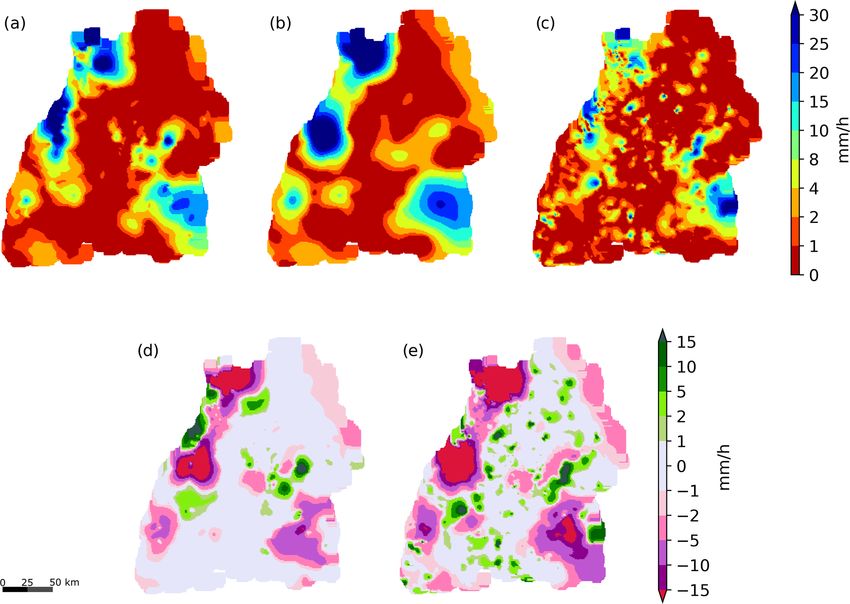
tion in this study. Figure 12 shows the maps corresponding There are already several approaches to using the precipi-
to the precipitation from 00:00 to 24:00 LT on 14 May 2018. tation data from PWSs (e.g. Chen et al., 2018; Cifelli et al.,
For this event, 515 PWS valid stations remained. This num- 2005), but they are generally based on daily data and simple
ber was reduced to 499 after the EBF. The behaviour of the QC approaches. Studies using more sophisticated QC work-
interpolations is similar to the 1 h cases shown above; the flows for hourly or sub-hourly precipitation data from PWSs
unfiltered and untransformed secondary interpolation is ir- are still limited. The approach presented by de Vos et al.
regular and shows a systematic underestimation. Due to the (2019) uses a comparison of the data with those of the nearby
higher temporal aggregation, the local differences have less stations to remove unreasonable values, with a separate pro-
of a contrast than in the case of the hourly maps. The combi- cedure for identifying and removing false zeros and another
nation contains more details, and the transition between high- filter for finding unreasonably high values. Subsequently, the
and low-intensity precipitation is more complex. The differ- bias is corrected by comparing past local observations to
ence between the primary (Fig. 12b) and the combination- a high-quality merged radar and point observation product.
based interpolation in Fig. 12a is relatively smaller than for The bias correction is performed uniformly in neighbour-
Hydrol. Earth Syst. Sci., 25, 583–601, 2021 https://doi.org/10.5194/hess-25-583-2021You can also read