NOSE AUGMENT: FAST AND EFFECTIVE DATA AUG-MENTATION WITHOUT SEARCHING
←
→
Page content transcription
If your browser does not render page correctly, please read the page content below
Under review as a conference paper at ICLR 2021

NOSE AUGMENT: FAST AND E FFECTIVE DATA AUG -
MENTATION W ITHOUT S EARCHING

 Anonymous authors
 Paper under double-blind review

                                           A BSTRACT
         Data augmentation has been widely used for enhancing the diversity of train-
         ing data and model generalization. Different from traditional handcrafted meth-
         ods, recent research introduced automated search for optimal data augmentation
         policies and achieved state-of-the-art results on image classification tasks. How-
         ever, these search-based implementations typically incur high computation cost
         and long search time because of large search spaces and complex searching algo-
         rithms. We revisited automated augmentation from alternate perspectives, such as
         increasing diversity and manipulating the overall usage of augmented data. In this
         paper, we present an augmentation method without policy searching called NOSE
         Augment (NO SEarch Augment). Our method completely skips policy search-
         ing; instead, it jointly applies multi-stage augmentation strategy and introduces
         more augmentation operations on top of a simple stochastic augmentation mecha-
         nism. With more augmentation operations, we boost the data diversity of stochas-
         tic augmentation; and with the phased complexity driven strategy, we ensure the
         whole training process converged smoothly to a good quality model. We con-
         ducted extensive experiments and showed that our method could match or surpass
         state-of-the-art results provided by search-based methods in terms of accuracies.
         Without the need for policy search, our method is much more efficient than the
         existing AutoAugment series of methods. Besides image classification, we also
         examine the general validity of our proposed method by applying our method to
         Face Recognition and Text Detection of the Optical Character Recognition (OCR)
         problems. The results establish our proposed method as a fast and competitive
         data augmentation strategy that can be used across various CV tasks.

1   INTRODUCTION
Data is an essential and dominant factor for learning AI models, especially in deep learning era
where deep neural networks normally require large data volume for training. Data augmentation
techniques artificially create new samples to increase the diversity of training data and in turn the
generalization of AI models. For example, different image transformation operations, such as ro-
tation, flip, shear etc., have been used to generate variations on original image samples in image
classification and other computer vision tasks. More intricate augmentation operations have also
been implemented, such as Cutout (Devries & Taylor, 2017), Mixup (Zhang et al., 2018), Cutmix
(Yun et al., 2019), Sample Pairing (Inoue, 2018), and so on. How to formulate effective augmenta-
tion strategies with these basic augmentation methods becomes the crucial factor to the success of
data augmentation.
Recent works (Cubuk et al., 2019; Lim et al., 2019; Ho et al., 2019) introduced automated searching
or optimization techniques in augmentation policy search. The common assumption of these meth-
ods is: a selected subset of better-fit augmentation policies will produce more relevant augmented
data which will in turn result in a better trained model. Here the augmentation policy is defined
by an ordered sequence of augmentation operations, such as image transformations, parameterized
with probability and magnitude. Though these methods achieved state-of-the-art accuracies on im-
age classification tasks, they lead to high computational cost in general, due to large search space
and extra training steps. More importantly, it is worth exploring whether it is really necessary to
find the best-fit subset of policies with specific parameter values of probability and magnitude. Ran-
dAugment (Cubuk et al., 2020) has started to simplify the parameters and scale down the search

                                                  1
Under review as a conference paper at ICLR 2021

space defined by AutoAugment Cubuk et al. (2019), but their method still relied on grid search for
iterative optimization of the simplified parameters.
Our method aims to fully avoid policy search and cost, meanwhile to maintain or improve model
performance in terms of both accuracy and training efficiency. Our work showed that by applying
simple stochastic augmentation policies with the same sampling space and other settings of training,
we could obtain equal or very close performance with search-based augmentation methods. Another
advantage of stochastic policies is that adding more operations in the pool does not bring additional
cost; while in search-base methods, more operations in the pool causes exponential increase of
the search space. Therefore, the second part of our method is to add more operations to the pool to
bring more data diversity. In practice, we introduced a new category of operations such as mixup and
cutmix into the operation pool. Furthermore, we tackled automated augmentation from overall data
usage point of view, in contrast to data creation point of view accentuated by policy-search based
methods. Inspired by the idea of Curriculum Learning (CL) (Bengio et al., 2009), which presents
training samples in an increasing order of difficulties, our method defines various complexity levels
of augmentation strategies and applies them with orders on phased training stages. To avoid the
confounding overfitting problem of original Curriculum Learning in practice, our method applies
the inverted order of Curriculum Learning, which presents the hardest augmentation strategies from
the beginning and gradually decreases the complexity levels.
In general, our augmentation method replaces policy search with stochastic policy generation, upon
which it introduces more operations for better diversity and phased augmentation strategy with de-
creasing complexities for a smooth learning convergence, and as an integral solution it achieves
better results. Figure 1 describes our method and the difference compared to search-based methods.

              Operation Pool                                         Searched
                   ( N ops )          Policy Search                   Policies                   Model Training
               ✔    op 1
               ✔    op 2                  Search                                             Augmentation Complexity
                     ...                Iterations                                                 (Constant)
               ✔    op N

                                 (a) Existing search based automated augmentation approach

              Operation Pool
               (N   + M ops )
                                                                                                 Model Training
                                       Random Policies
               ✔op 1
               ✔op 2
                 ...                                                                         Augmentation Complexity
              ✔ op N                                                                              (Decreasing)
              ✔ op N + 1
              ✔ op N + 2
                   ...
              ✔ op N + M

                                 (b) Our NOSE augment without policy search

                     Figure 1: No Search (NOSE) Augment vs Search-based Augment

The main contributions of this paper can be summarized as follows:

1. We present a no-search (NOSE) augmentation method as an alternative of computation-intensive
search-based auto-augment methods. By jointly applying phased augmentation strategy and intro-
ducing more augmentation operations on top of a simple stochastic augmentation mechanism, NOSE
augment achieves state-of-the-art (SOTA) accuracies on CIFAR 10, CIFAR 100 (Krizhevsky, 2009)
and close-to-SOTA results on other benchmark datasets. Our ablation study demonstrates that all
the components of our methods should be combined together to achieve the best performance.
2. We demonstrate that a stochastic-based augmentation approach can obtain accuracies comparable
to those of search-based methods while achieving overwhelming advantage on overall augmentation
and training efficiency as the searching phase is completely avoided.
3. Besides image classification, we also applied NOSE augment on face recognition and text de-
tection (OCR) tasks, and obtained competitive or better results in comparison with search-based
methods. This further proves the advantage and generality of NOSE augment.

                                                                2
Under review as a conference paper at ICLR 2021
2 RELATED WORKS
Our work is most closely related to RandAugment (Cubuk et al., 2020). A key idea in RandAugment
is to avoid a separate search phase on proxy datasets but chose instead to reduce the search space
by decreasing the number of parameters. For instance, the probability for each operator is set to a
constant uniform probability. The two sets of data augmentation parameters to be searched are N,
the number of transformations for a given image and M, the discrete operator magnitude. These two
parameters are regarded as hyperparameters and tuned using grid search. Our method is similar to
RandAugment in terms of the operators used and the setting of equal probability for each operator.
The most contrasting difference between RandAugment and our method is that RandAugment is
still a search-based method with search cost while our method skips policy search completely and
tackles the problem by introducing new augmentation operations and further new strategies built
upon stochastic policies.
Our work stands diametrically opposite to the AutoAugment series of methods (Cubuk et al., 2019;
Lim et al., 2019; Zhang et al., 2020), in which the best data augmentation policy is derived through
a search. AutoAugment (Cubuk et al., 2019) uses a RNN controller to propose an augmentation
strategy. Based on this proposed augmentation strategy, the model is trained and use the resulting
validation accuracy to update the RNN controller. Although AutoAugment achieves good results
on the standard benchmark datasets, the search cost is prohibitively huge, for instance, 5000 GPU
(NVIDIA Tesla P100) hours on the CIFAR-10 dataset and Pyramid-Net+ShakeDrop model.
Fast AutoAugment (Fast AA) (Lim et al., 2019) ameliorates AutoAugment’s huge search cost with
a three pronged approach. Smaller datasets are used for policy search. The idea of density matching
is proposed to avoid having to re-train the model for assessing the validation accuracy for each
proposed policy. The use of Bayesian Optimization based method (Bergstra et al., 2011) also helps
to converge to an effective augmentation policy quickly. Adversarial Augment (Adv AA) (Zhang
et al., 2020) reduces the huge computational cost of AutoAugment through the adversarial policy
framework, which generates data samples that maximizes the training loss of the target network.
PBA (Ho et al., 2019) introduces the idea of non-stationary policy schedules instead of the fixed
augementation policy proposed in AutoAugment. The non-stationary policy schedules refers to how
the policy evolves with the training epochs.
Our main differences with aforementioned state-of-the-art methods lie in our stochastic policy de-
scribed in section 3.1 and the multi-stage complexity driven augmentation policy outlined in section
3.3. We use the same set of operators and settings as these related works.
3 METHOD
We describe the three key components of our proposed method in this section. In section 3.1, we
put forward a stochastic-based method as opposed to the search-based paradigm advocated by many
of the state-of-the-art works described in section 2. Due to the counter-intuitiveness (but effective)
nature of this stochastic-based method, we first provide insights and motivations into stochastic
augmentation policies in section 3.1. In section 3.2, we capitalize on our proposed stochastic-based
method by proposing additional operators that will further enrich the data augmentation diversity,
since there is no extra search cost for adding new operators with a no-search method. In 3.3, we
propose a multi-stage complexity driven policy that helps to resolve the tension between augmented
data diversity and data distribution fidelity. Our ablation study demonstrates that the performance of
our method is not a simple incremental benefit with each individual component, but rather, the three
components need to work together to achieve a competitive performance with no policy search cost.
3.1 STOCHASTIC POLICY - SKIPPING POLICY SEARCH
The first component of our method removes policy searching completely and applies a stochastic
augmentation policy with randomly selected operations and magnitudes. Unlike the search-based
methods, once an operation is selected, it is used with 100% probability. Our stochastic method
follows the same policy definition as existing search-based methods. Specifically, one augmentation
policy has 5 sub-policies; each sub-policy consists of 2 augmentation operations. The base operation
pool includes the following 15 operations: ShearX/Y, TranslateX/Y, Rotate, AutoContrast, Invert,
3Under review as a conference paper at ICLR 2021
Equalize, Solarize, Posterize, Contrast, Color, Brightness, Sharpness and Cutout. Each operation
has 11 uniformly discretized magnitudes which is randomly selected upon each use.
We provide an abstract analysis for stochastic policy through a data deficiency complement point
of view, in which a relatively slower accuracy increase is expected for stochastic method in early
stage of training. We refer to the time period required by stochastic approach to accumulate enough
amount of data in the deficient dimensions as the Stochastic Accumulation Stage (SAS). However, as
training carries on, the amount of data of deficient dimension in the random approach may gradually
get close to or even go beyond the one in search-based methods. When enough number of epochs
is reached, the performance of random policy may match or even overtake search-based methods.
More detailed intuitions are provided in section A.1 of the appendix.
Note that we are not claiming that this stochastic policy outperforms the search-based augmentation
policies, but rather, this stochastic policy provides a good foundation for us to build upon; it allows
us to further incorporate additional operators and a multi-stage complexity augmentation strategy
with very little or no extra cost compared to search-based methods.
3.2 INTRODUCING ADDITIONAL AUGMENTATION OPERATIONS
In our method, we introduce mix-based operations such as mixup, cutmix, and augmix (Hendrycks
et al., 2020) in addition to the randomly generated augmentation policies. RandAugment showed
certain operation (e.g. posterize) brought consistent negative effect to augmentation result regardless
of the number of operations in the pool; while some (e.g. rotate) had consistent positive effect. We
also observed some operations might harm the augmentation performance when directly applied on
stochastic method; however, an interesting finding is that the negative influence could be weakened
or even turned back to positive when these operations were used together with our complexity driven
strategy, which is explained in next section.
Note that these mix-based operators can also be introduced to the search-based methods. The main
difference is that there is no extra overhead or cost as far as our method is concern; whereas these
additional operators will incur even larger cost for an already expensive search process.
3.3 AUGMENTATION WITH MULTI-STAGE COMPLEXITY DRIVEN STRATEGY
Curriculum learning (CL) puts forward the view that learning progressively harder tasks may im-
prove training performance. Drawing inspiration from their work, we manipulate the overall data
complexity in different training stages instead of controlling the creation of static augmentation poli-
cies. The data complexity here refers to the distortion produced by the data augmentation operators
and the result of successive applications of these operators. In our work, these augmentation opera-
tors are first grouped into three categories: 1) baseline operators such as flip, random crop, and cutout
which are frequently used as fundamental augmentations for image-related tasks; 2) mix-based op-
erations such as mixup, cutmix, and augmix; and 3) transformation-based operators such as rotate,
shear, sharpness etc., which have been used in experiments of related works (Cubuk et al., 2019;
2020; Lim et al., 2019; Zhang et al., 2020). Our method then divides the complexity of augmenta-
tion into multiple levels that map to various combinations of the above three categories, and apply
them in different training stages. Starting from the simplest, three complexity levels are defined as
follow. First, baseline augmentation (BaseAug), exactly the same baseline augmentation used in
AutoAugment; depending on the specific datasets, BaseAug may consist of flip, random crop, or
cutout operations in the baseline category. Second, advanced augmentation (AdAug), which intro-
duces the category of mix-based operations upon BaseAug. Third, super augmentation (SupAug),
which additionally applies 15 transformation operators upon AdAug. Except for baseline augmen-
tations which are applied with 100% probability, mix-based and transformation augmentations are
selected in a stochastic manner when the corresponding augmentation category is applied in a certain
augmentation stage.
For the overall augmentation strategy, we first tried applying augmentation complexity in ascending
order while the training proceeded, same as Curriculum Learning. However, the result was not ideal
and we noticed apparent trend of over-fitting in training. Our interpretation of the phenomenon is
that the over-fitting is due to insufficient diversity of training data. When this insufficiency takes
place in early training stages of a deep neural network (DNN), it is prone to over-fit because the
4Under review as a conference paper at ICLR 2021
---------------
0.9 stage3
stage2
-------
--
3
----
0.8 stage1
-------------------------------
Train Loss
Test Accuracy
------------------
2 0.7
------------------------------
----
stage1 0.6
1 -----
-----
stage2 0.5
----
stage3
0 0.4
0 40 80 120 160 200 240 0 40 80 120 160 200 240
Epoch Epoch
(a) Training loss with 3-phase augmentation (b) Test accuracy (best) with 3-phase augmentation
Figure 2: Phased Augmentation
relatively smaller amount of data with limited diversity cannot support learning DNNs with large
sizes and complex structures.
Above-mentioned observation led us to apply the inverted CL order of augmentation complexities,
which trains the network with sufficiently diversified data in the early stage and gradually adapts the
network to the original data distribution without augmentation. Specifically, our method removes
one augmentation category going from one stage to the next e.g. the transformation category is
removed going from stage 1 to stage 2. Note that our method does not tune or search the optimal
epoch allocation during this process, it has a common setting of epoch allocation for a three-phase
augmentation strategy. Here the first stage is set to have the highest complexity and the majority of
the epochs, it is necessary to maintain the high complexity and enough epochs to obtain sufficient
data diversity and prevent overfitting. Details of phase definition are further described in Section 4,
and our experiments verified our hypothesis and confirmed the effectiveness of this method. Figure
2 shows example curves of training loss and test accuracy with a three-stage augmentation strategy
obtained in practice; jumps can be seen on boundaries of adjacent stages.
We can also explain the need for data diversity vs. fidelity to the original data distribution in terms
of the data augmentation theoretical foundation constructed in (Dao et al., 2019). In this work, data
augmentation is regarded as a perturbation about the original data. Thus, using a Taylor expansion
about the original data, the first order effect of data augmentation is given in equation 1. From
equation 1, we can therefore understand data augmentation as feature averaging over the data aug-
mentation operators. This is precisely the reason why towards the end of training, we want to keep
only data augmentation operators that introduce minimum distortion, thus allowing convergence to
a model that can best learn the original data distribution, instead of the augmented distribution.
n
1X
g(w) ≈ ĝ(w) := l(wT Eti ∼T (xi ) [φ(ti )]; yi ) (1)
n i=1
where g(.) is the loss function after data augmentation, l(.) is the original loss function, w are the
weights to be learned, ti is the data augmentation operator sampled from the operator pool T , ĝ(.)
is the expansion at any data point not dependent on ti , φ is the feature map and yi is the label.
The second order expansion is given in equation 2. The squared term in equation 2 gives a clear
indication of the role of data augmentation towards variance regularization, helping to prevent over-
fitting. This gives strong justification to why we chose higher complexity data augmentation op-
erators in the early part of the training, which serves to provide strong regularization effect for
preventing choosing w that will lead to over-fitting in the latter part of training.
n
1 X h
T 2 00 T
i
g(w) ≈ ĝ(w) + Eti ∼T (xi ) w (φ(ti ) − ψ(ti )) l (ζi (w φ(ti )); yi ) (2)
2n i=1
5Under review as a conference paper at ICLR 2021
where ψ(xi ) = Eti ∼T (xi ) [φ(ti )] is the expectation of the original feature map over the data augmen-
00
tation operators and l (.) is the remainder function from Taylor’s theorem. For more mathematical
details, we highly recommend the readers to refer to (Dao et al., 2019).
Each of the above-mentioned three sub-methods may benefit augmentation individually; however
the best result is achieved by combining them together as one solution, NOSE augment, whose
performance is demonstrated with our experiments presented as follows.
4 EXPERIMENTS AND RESULTS
In this section, we first evaluate the performance of NOSE augment in terms of accuracy and ef-
ficiency on CIFAR-10/CIFAR-100, Reduced CIFAR-10 which includes 4K training samples (ran-
domly chosen), SVHN (Netzer et al., 2011) and ImageNet (Deng et al., 2009). NOSE achieves
state-of-the-art results on many datasets or models, and competitive ones on the rest. We compare
our method with our baseline and existing search-based methods described in section 2, namely
AutoAugment, Fast AA, RandAugment, Adv AA and demonstrates both the efficiency and effec-
tiveness of our method. We then present our extensive experiments on sub-methods of NOSE and
ablation studies. Besides image classification tasks, we further conduct experiments on Face Recog-
nition and Text Detection tasks, which further demonstrate the transferability of our method across
domains.
4.1 OVERALL EXPERIMENT SETUP
As presented in Section 3, NOSE relies on three sub-methods including stochastic policies, extra
operations, and staged augmentation strategy. One stochastic policy is composed of 2 operations,
which are randomly selected from the base operation pool as described in Section 3.1. Each oper-
ation randomly takes one of the 11 discretized magnitudes which uniformly space between 0 and 1
when it is used. Once the operation is selected, it is applied with 100% probability. Upon stochastic
policies, mix-based operations including Mixup, Cutmix, and Augmix are added into the opera-
tion pool. Augmix is applied on individual images when selected, same as existing operations in
the pool; while Mixup and Cutmix are randomly applied on individual batches due to the inherent
pairing logic of these operations. We then applied 3 stages of augmentation along training, as men-
tioned in Section 3.3. For the first stage, we augment the training data with the highest complexity
(SupAug); followed by the 2nd stage with slightly lower complexity (AdAug); and finally the third
stage with the lowest complexity (BaseAug). We examined NOSE with extensive experiments on
multiple datasets listed below. Please refer to section A.3 for the training details. We follow Au-
toAugment and successive related works for baseline settings, we provide our reproduced baseline
results together with those reported by AutoAugment in Table 1.
4.2 EXPERIMENTS ON ACCURACY
As shown in Table 1, our NOSE augment is able to achieve competitive accuracies on most datasets
and models compared to other SOTA works. In particular, NOSE augment obtains 0.56% SOTA ac-
curacy improvement with Wide-ResNet-40-2 on CIFAR-10, while on CIFAR-100 it obtains 0.87%
SOTA increment with Wide-ResNet-40-2 and 0.44% SOTA increment with Wide-ResNet-28-10.
Moreover, for all models trained on reduced CIFAR-10, NOSE augment achieves the highest scores
when compared to AutoAugment, PBA and RandAugment. On ImageNet, NOSE achieve 0.65% ac-
curacy increment compared to most search-based methods (AutoAugment, Fast AA, RandAugment)
except Adv AA.
4.3 EXPERIMENTS ON EFFICIENCY
This experiment examines the efficiency of NOSE augment and compares the results with search-
based methods. The computation cost in this context has two major components: searching (or
tuning) cost and training cost. For the searching part, the cost of a search-based method is normally
proportional to some factors such as model size, dataset size, number of the operations in augmen-
tation pool etc. For example, Fast AA’s policy-search cost is 3.5 GPU-hours for wresnet 40-2 with
reduced Cifar-10, but 780 GPU-hours for Pyramid-Net+ShakeDrop on full Cifar-10 dataset. Table 2
6Under review as a conference paper at ICLR 2021
Table 1: Top1 test accuracy(%) on various datasets and models. Our baseline follows the same
baseline settings of AutoAugment; the first two columns show our reproduced baseline results and
the ones reported by AutoAugment respectively.
DataSet Model Baseline(our) Baseline(AA) Cutout AA PBA FastAA RA AdvAA Ours
Wide-ResNet-40-2 94.52 94.70 95.90 96.30 - 96.30 - - 96.86
Wide-ResNet-28-10 95.43 96.10 96.90 97.40 97.40 97.30 97.30 98.10 97.97
CIFAR-10 Shake-Shake(26 2x32d) 95.78 96.40 97.00 97.50 97.50 97.50 - 97.64 97.54
Shake-Shake(26 2x96d) 96.65 97.10 97.40 98.00 98.00 98.00 98.00 98.15 98.3
Shake-Shake(26 2x112d) 96.68 97.20 97.40 98.10 98.00 98.10 - 98.22 98.31
PyramidNet+ShakeDrop - 97.30 97.70 98.50 98.50 98.30 98.50 98.64 98.57
Wide-ResNet-28-2 80.10 - 81.94 85.60 - - 85.30 - 87.38
Reduced CIFAR-10 Wide-ResNet-28-10 81.17 81.20 83.50 87.70 87.18 - 86.80 - 89.18
Shake-Shake(26 2x96d) 80.26 82.90 86.60 89.98 89.25 - - - 89.98
Wide-ResNet-40-2 74.18 74.00 74.80 79.30 - 79.40 - - 80.27
CIFAR-100 Wide-ResNet-28-10 80.79 81.20 81.60 82.90 83.30 82.70 83.30 84.51 84.95
Shake-Shake(26 2x96d) 79.77 82.90 84.00 85.70 84.70 85.40 - 85.90 85.31
SVHN (core set) Wide-ResNet-28-10 96.57 96.90 - 98.10 - - 98.30 - 98.06
IMAGENET ResNet50 - 76.30 - 77.60 - 77.60 77.60 79.40 78.52
shows the searching costs of different augmentation methods. Here, Adv AA claimed its search cost
close to 0 as it does not have a separate policy search phase, but its training cost is much higher than
our method, which is further explained as follow. For the training part, NOSE augment has similar
cost with the majority of search-based methods like AutoAugment and Fast AA, which process the
training samples in one round. Suppose the training cost is a constant value C, which is affected by
the dataset size and the number of total training epochs. For Adv AA, the training cost is at least
8 times C, because it augments more data in one epoch (number of batches is 8 times compared to
NOSE, AutoAugment, and Fast AA). Rand Augment has significantly reduced the search space to
10x10, but it still relies on grid search with training and has a relatively higher training cost than
NOSE augment. In general, our method has the overwhelming advantage in terms of the overall ef-
ficiency as it bypasses policy search completely and does not increase training cost with any tuning
or optimization logic.
Table 2: Efficiency on various dataset. Unit: GPU hour; hardware: Fast AA - Tesla V100, AutoAug-
ment - Tesla P100, PBA - Titan XP. Dashes indicate unavailable figures; despite the unavailability,
the advantage of our method in terms of search cost is apparent.
Search Cost
Method Search Space Reduced CIFAR-10 CIFAR-10 Reduced ImageNet
(Wide-ResNet-40-2) (PyramidNet) (Wide-ResNet-40-2)
AA 1032 5000 - 15000
FastAA 1032 3.5 780 450
PBA 1061 5 - -
Our 0 0 0 0
4.4 EXPERIMENTS ON STOCHASTIC POLICIES
This experiment presents potential factors that could influence the performance of stochastic poli-
cies. The factors we explore are: 1) number of operations per sub-policy; 2) number of total oper-
ations in the augmentation operation pool. Experiment results of the first factor showed that when
the number of operations in a sub-policy is larger than 3, the downgrade in performance is clear;
our interpretation is that overlapped operations beyond certain threshold may cause downgrade in
image quality which will in turn affect the augmentation performance negatively. Similar to what
RandAugment found in their experiment, our experiment results for the second factor revealed that
in general more operations in the candidate pool can benefit augmentation as it brings more data di-
versity, which inspire us to introduce additional operations in our method. For further details, please
refer to the section A.4.
7Under review as a conference paper at ICLR 2021
4.5 EXPERIMENTS ON MULTI-STAGE AUGMENTATION STRATEGY
As described in section 3.3, our data augmentation consists of three stages: stage 1 (SupAug), stage
2 (AdAug), stage 3 (BaseAug). We first look at the effect of two stages vs. three stages. The two
stage strategy is constructed by choosing two of the three stages. From Table 3a, we see that while
”stage 1 + stage 3” has the best two stage performance, our three stage augmentation strategy still
offers the best overall performance. The importance of having the minimal distortion stage 3 is also
emphasized from the observation of a sharp accuracy drop for the ”stage 1 + stage 2” combination.
Next we look at the epoch allocation for each stage. We vary the number of epochs for each stage on
the CIFAR-100 dataset. From Table 3b, we derive an overall principle for epoch allocation: stage 1
needs to have the majority of the epoch, about 85% from our experiment; and stage 2 and 3 are set
as 10% and 5% respectively. This is used as common strategy and one-time setting for all cases; no
tuning or searching is used in our method for epoch allocation. The total number of epochs for all
experiments in this section is set to 200. Figure 6 in the appendix shows the training loss profile for
these different epoch allocation.
We also justify the need for an inverted CL by comparing with the standard CL, where the augmen-
tation stages go from simple to complex. As shown in Table 4, there is a noticeable performance
drop associated with standard CL (simple to complex), compared to our proposed inverted CL.
Table 3: Multi-stage augmentation study on 2 vs. 3 stages and epoch allocation for each stage.
Stage 1 Stage 2 Stage 3 Accuracy
Stage Stage Stage Stage
50 100 50 78.37
1,2 1,3 2,3 1,2,3
50 50 100 77.92
CIFAR-10 93.01 97.44 96.94 97.75 70 70 60 77.98
CIFAR-100 73.89 79.33 77.78 79.89 170 20 10 79.89
(a) A comparison of two stage vs. our proposed three (b) Accuracy on the CIFAR-100 dataset by vary-
stage augmentation strategy accuracy on the CIFAR-10 ing epoch allocation for each stage
and CIFAR-100, using Wide-ResNet-40-2 and Wide-
ResNet-28-10 respectively
Table 4: Low to high complexity (increasing image distortion).
DataSet Model Simple To Complex Ours
CIFAR-10 Wide-ResNet-28-10 92.76 97.75
CIFAR-100 Wide-ResNet-40-2 72.6 79.89
4.6 EXPERIMENTS ON FACE RECOGNITION
Face recognition system is trained using the CASIAWebFace (Yi et al., 2014) dataset. CASIA
dataset contains 10575 subjects and around 500k face images of the subjects. We used the test
sets of LFW (Huang et al., 2008), AgeDB-30 (Moschoglou et al., 2017) and CFP-FP (S. Sengupta,
2016). The training details of our experiments for face recognition task are given in section A.6. As
shown in Table 5a our model improved over the baseline result and showed similar accuracy results
compared to Fast AA; while our method achieves much better training efficiency.
4.7 EXPERIMENTS ON TEXT DETECTION
We conducted experiments on ICDAR 2017 MLT dataset (Nayef et al., 2017) to test the generality
of our method for text detection tasks. We trained our implementation of EAST (Zhou et al., 2017)
model with 3 different augmentation strategies. The training details of our experiments for text
detection task are given in section A.7. We performed several independent runs and averaged the
results that are shown in Table 5b. In addition, we also included the results of our customized metric
for each trained model to show its consistency. Further details about the customized metric which
we call it as E-Score are given in section A.7. According to the final results, our approach showed
8Under review as a conference paper at ICLR 2021
Table 5: Face recognition and text detection results
Default Fast AA Ours Default Fast AA Ours
F1 50.36 50.51 54.27
LFW 99.20 99.27 99.25 Precision 44.64 44.1 50.96
AgeDB-30 91.82 91.88 91.92 Recall 57.76 59.1 58.04
Avg. Precision 46.58 48.29 48.35
CFP-FP 94.31 95.53 95.17 E-Score 1.44 1.46 1.47
(a) Face recognition accuracy on the standard bench- (b) Text detection results on the ICDAR MLT 2017
mark dataset dataset. Note that E-Score is our customized metric.
better performance than other approaches, with the model trained using our approach gains ∼4%
advantage on the final F1 score compared to the model trained by default training approach with
using baseline augmentations and the model trained by using the augmentation policies found via
Fast AA.
4.8 ABLATION EXPERIMENTS
We design ablation studies to explore the benefits brought by individual components of our pro-
posed method. The first control experiment evaluates stochastic policy (”Stoch. + Base”), in which
transformation augmentations are applied randomly on top of baseline augmentations while mix-
based operations and stage concept are removed. The second control experiment evaluates phased
augmentation strategy without mix-based augmentations (”Stoch. + 2-stage”), where the first stage
consists of stochastic transformations on top of baseline augmentations and the second stage with
only the baseline augmentations. Note that 2-stage but not 3-stage is used here because remov-
ing mix-based augmentations removes the corresponding phase, stochastic augmentations have to
be kept otherwise there will be only one stage left. The third control experiment evaluates the mix-
based operations on top of stochastic transformations without phased augmentation strategy (”Stoch.
+ mix-based”). As we can see from Table 6, using partially selected components of our proposed
method results in apparent accuracy drops in all cases, thus validating that our method as a whole is
greater than the sum of its parts.
Table 6: Ablation study result. In ”Stoch. + 2-stage”, the first stage consists of stochastic trans-
formations on top of baseline augmentations and only the baseline augmentations for the second
stage.
Model Stoch.+ Base Stoch.+ 2-stage Stoch.+ mix-based Ours
CIFAR-10 Wide-ResNet-40-2 96.28 96.3 92.87 97.94
Wide-ResNet-28-10 97.43 97.51 96.49 97.75
CIFAR-100 Wide-ResNet-40-2 79.12 79.34 72.56 79.89
Wide-ResNet-28-10 82.61 83.11 79.49 85.17
5 CONCLUSION AND DISCUSSION
In this paper, we present an automated augmentation method without policy search. Upon stochastic
policies, our method introduces more augmentation methods without extra search cost; by further
applying a multi-stage complexity driven augmentation strategy, our method achieved state-of-the-
art accuracies for image classification task on most datasets and absolute advantage on efficiency as
policy search is skipped. We also apply this method on face recognition and text detection tasks,
thereby demonstrating the generality of our method. Despite the strong performance of our proposed
method, we are not denigrating the search-based methods and downplaying their values. On the
contrary, we believe search-based methods can be further improved with revised or different search
spaces. One of our future works is applying automated search techniques on our method for new
augmentation operation selection and staged augmentation strategy optimization.
9Under review as a conference paper at ICLR 2021
R EFERENCES
Yoshua Bengio, J. Louradour, Ronan Collobert, and J. Weston. Curriculum learning. In ICML ’09,
2009.
J. Bergstra, R. Bardenet, Yoshua Bengio, and B. Kégl. Algorithms for hyper-parameter optimization.
In NIPS, 2011.
Bor-Chun Chen, Chu-Song Chen, and Winston H Hsu. Cross-age reference coding for age-invariant
face recognition and retrieval. In European conference on computer vision, pp. 768–783. Springer,
2014.
Sheng Chen, Yang Liu, Xiang Gao, and Zhen Han. Mobilefacenets: Efficient cnns for accurate
real-time face verification on mobile devices. In Chinese Conference on Biometric Recognition,
pp. 428–438. Springer, 2018.
Yunjey Choi, Min-Je Choi, Munyoung Kim, Jung-Woo Ha, Sunghun Kim, and Jaegul Choo.
Stargan: Unified generative adversarial networks for multi-domain image-to-image translation.
CoRR, abs/1711.09020, 2017. URL http://arxiv.org/abs/1711.09020.
E. Cubuk, Barret Zoph, Dandelion Mané, V. Vasudevan, and Quoc V. Le. Autoaugment: Learning
augmentation strategies from data. 2019 IEEE/CVF Conference on Computer Vision and Pattern
Recognition (CVPR), pp. 113–123, 2019.
E. D. Cubuk, Barret Zoph, Jonathon Shlens, and Quoc V. Le. Randaugment: Practical automated
data augmentation with a reduced search space. 2020 IEEE/CVF Conference on Computer Vision
and Pattern Recognition Workshops (CVPRW), pp. 3008–3017, 2020.
Tri Dao, A. Gu, Alexander J. Ratner, V. Smith, C. D. Sa, and C. Ré. A kernel theory of modern data
augmentation. Proceedings of machine learning research, 97:1528–1537, 2019.
Jia Deng, W. Dong, R. Socher, L. Li, K. Li, and Li Fei-Fei. Imagenet: A large-scale hierarchical
image database. In CVPR 2009, 2009.
Jiankang Deng, Jia Guo, and Stefanos Zafeiriou. Arcface: Additive angular margin loss for deep face
recognition. CoRR, abs/1801.07698, 2018. URL http://arxiv.org/abs/1801.07698.
Terrance Devries and Graham W. Taylor. Improved regularization of convolutional neural networks
with cutout. ArXiv, abs/1708.04552, 2017.
Xavier Gastaldi. Shake-shake regularization. ArXiv, abs/1705.07485, 2017.
D. Han, J. Kim, and J. Kim. Deep pyramidal residual networks. In 2017 IEEE Conference on
Computer Vision and Pattern Recognition (CVPR), pp. 6307–6315, 2017. doi: 10.1109/CVPR.
2017.668.
K. He, X. Zhang, S. Ren, and J. Sun. Deep residual learning for image recognition. In 2016
IEEE Conference on Computer Vision and Pattern Recognition (CVPR), pp. 770–778, 2016. doi:
10.1109/CVPR.2016.90.
Dan Hendrycks, Norman Mu, E. D. Cubuk, Barret Zoph, J. Gilmer, and Balaji Lakshminarayanan.
Augmix: A simple data processing method to improve robustness and uncertainty. ArXiv,
abs/1912.02781, 2020.
D. Ho, Eric Liang, I. Stoica, P. Abbeel, and Xi Chen. Population based augmentation: Efficient
learning of augmentation policy schedules. In ICML, 2019.
Gary B Huang, Marwan Mattar, Tamara Berg, and Eric Learned-Miller. Labeled faces in the wild:
A database forstudying face recognition in unconstrained environments. 2008.
H. Inoue. Data augmentation by pairing samples for images classification. ArXiv, abs/1801.02929,
2018.
10Under review as a conference paper at ICLR 2021
Kye-Hyeon Kim, Yeongjae Cheon, Sanghoon Hong, Byung-Seok Roh, and Minje Park. PVANET:
deep but lightweight neural networks for real-time object detection. CoRR, abs/1608.08021, 2016.
URL http://arxiv.org/abs/1608.08021.
A. Krizhevsky. Learning multiple layers of features from tiny images. 2009.
Sungbin Lim, Ildoo Kim, Taesup Kim, Chiheon Kim, and Sungwoong Kim. Fast autoaugment. In
Advances in Neural Information Processing Systems 32, pp. 6665–6675. 2019.
Canjie Luo, Yuanzhi Zhu, Lianwen Jin, and Yongpan Wang. Learn to augment: Joint data augmen-
tation and network optimization for text recognition. In CVPR, 2020.
Stylianos Moschoglou, Athanasios Papaioannou, Christos Sagonas, Jiankang Deng, Irene Kotsia,
and Stefanos Zafeiriou. Agedb: the first manually collected, in-the-wild age database. In Pro-
ceedings of the IEEE Conference on Computer Vision and Pattern Recognition Workshops, pp.
51–59, 2017.
N. Nayef, F. Yin, I. Bizid, H. Choi, Y. Feng, D. Karatzas, Z. Luo, U. Pal, C. Rigaud, J. Chazalon,
W. Khlif, M. M. Luqman, J. Burie, C. Liu, and J. Ogier. Icdar2017 robust reading challenge on
multi-lingual scene text detection and script identification - rrc-mlt. In 2017 14th IAPR Interna-
tional Conference on Document Analysis and Recognition (ICDAR), volume 01, pp. 1454–1459,
2017.
Yuval Netzer, T. Wang, A. Coates, Alessandro Bissacco, B. Wu, and A. Ng. Reading digits in natural
images with unsupervised feature learning. 2011.
Albert Pumarola, Antonio Agudo, Aleix M. Martı́nez, Alberto Sanfeliu, and Francesc Moreno-
Noguer. Ganimation: Anatomically-aware facial animation from a single image. CoRR,
abs/1807.09251, 2018. URL http://arxiv.org/abs/1807.09251.
C.D. Castillo V.M. Patel R. Chellappa D.W. Jacobs S. Sengupta, J.C. Cheng. Frontal to profile face
verification in the wild. In IEEE Conference on Applications of Computer Vision, February 2016.
YadiraF. Yadiraf/face3d. URL https://github.com/YadiraF/face3d.
Y. Yamada, M. Iwamura, Takuya Akiba, and K. Kise. Shakedrop regularization for deep residual
learning. IEEE Access, 7:186126–186136, 2019.
Dong Yi, Zhen Lei, Shengcai Liao, and Stan Z. Li. Learning face representation from scratch. CoRR,
abs/1411.7923, 2014. URL http://arxiv.org/abs/1411.7923.
Sangdoo Yun, Dongyoon Han, Seong Joon Oh, Sanghyuk Chun, Junsuk Choe, and Youngjoon
Yoo. Cutmix: Regularization strategy to train strong classifiers with localizable features. 2019
IEEE/CVF International Conference on Computer Vision (ICCV), pp. 6022–6031, 2019.
Sergey Zagoruyko and Nikos Komodakis. Wide residual networks. In Edwin R. Hancock Richard
C. Wilson and William A. P. Smith (eds.), Proceedings of the British Machine Vision Conference
(BMVC), pp. 87.1–87.12. BMVA Press, September 2016. ISBN 1-901725-59-6. doi: 10.5244/C.
30.87. URL https://dx.doi.org/10.5244/C.30.87.
Hongyi Zhang, M. Cissé, Yann Dauphin, and David Lopez-Paz. mixup: Beyond empirical risk
minimization. ArXiv, abs/1710.09412, 2018.
Xinyu Zhang, Qiang Wang, Jian Zhang, and Zhao Zhong. Adversarial autoaugment. In International
Conference on Learning Representations, 2020. URL https://openreview.net/forum?
id=ByxdUySKvS.
Xinyu Zhou, Cong Yao, He Wen, Yuzhi Wang, Shuchang Zhou, Weiran He, and Jiajun Liang.
EAST: an efficient and accurate scene text detector. CoRR, abs/1704.03155, 2017. URL http:
//arxiv.org/abs/1704.03155.
11Under review as a conference paper at ICLR 2021
A APPENDIX
A.1 STOCHASTIC POLICY INSIGHT
We provide a motivation for stochastic policy through a data deficiency complement point of view.
We think of the training data as a pool of knowledge or features with multiple dimensions. The
columns in the histogram indicate the volume of data with this knowledge dimension. With searched
static policies of AutoAugment methods (as shown in Figure 4a), the buckets of the most deficient
data dimensions (e.g. dimension 2 in the figure) can be filled fast once training starts and catch up
with other dimensions in a relatively short period. In contrast, data growing with random policies
are balanced amongst all dimensions in a larger sampling scope (Figure 4b), so data accumulation
on the dimensions of deficient data may be slower than search-based methods. Hence, in early stage
of training, a relatively slower accuracy increase is expected. We refer the time period required by
stochastic approach to accumulate enough amount of data in the deficient dimensions as Stochastic
Accumulation Stage (SAS).
However, the relative deficiency are changing over time along training (as shown in Figure 4a); with
static policies searched by algorithms such as AutoAugment and Fast AA, the constant increase
on the focused dimensions may not fit the dynamic state of training and the data augmentation on
the latest deficient dimensions slows down. Therefore, as training time goes, the data amount of
deficient dimension in random approach may gradually get close to or even go beyond the one in
search-based methods. When enough number of epochs is reached, the performance of random pol-
icy may match or overtake search-based methods. This prediction is verified by comparing practical
training results between stochastic method and Fast AA, as shown in Figure 3.
0.8 1.2
Fast AA
Fast AA
0.7 1 Stochastic
Stochastic
0.6
0.8
Test Accuracy
0.5
Test Loss
0.4 0.6
0.3
0.4
0.2
0.2
0.1
0 0
0 50 100 150 200 250 0 50 100 150 200 250
Epoch Epoch
(a) Test loss: WResNet-28-10 on (b) Test accuracy: WResNet-28-10
CIFAR-10 on CIFAR-10
2.5 0.9
0.8 Fast AA
Fast AA Stochastic
2 0.7
Stochastic
0.6
Test Accuracy
1.5
Test Loss
0.5
0.4
1
0.3
0.2
0.5
0.1
0
0 0 50 100 150 200 250
0 50 100 150 200 250 Epoch
Epoch
(c) Test loss: WResNet-40-2 on (d) Test accuracy: WResNet-40-2 on
CIFAR-100 CIFAR-100
Figure 3: Training with Augmentation: Stochastic VS Fast AA
Our hypothesis is confirmed with experiment results on multiple datasets, as shown in Figure 4. As
we can see in the figure, the SAS periods of stochastic method are shorter than the total epochs
spent on achieving optimal results in search-based methods, thus the slower accumulation of defi-
cient data with random policies can be ignored while the benefit is it completely skips the expensive
policy searching. We have to mention that succeeding research in Adversarial AutoAugment ex-
ploited adversarial network for generating dynamic policies which to some extent made up for the
disadvantages of static policies. But the time and cost of policy searching were still existing and
considerable, compared to the stochastic approach without any searching.
12Under review as a conference paper at ICLR 2021
First of all, our method removes policy searching completely and applies stochastic augmentation
policies with randomly selected operations and magnitudes. Once an operation is selected, it is used
with 100% probability. Our stochastic method follows the same policy definition as existing search-
based methods. Specifically, one augmentation policy has 5 sub-policies; each sub-policy consists
of 2 augmentation operations. The operation pool includes the following 15 operations: ShearX/Y,
TranslateX/Y, Rotate, AutoContrast, Invert, Equalize, Solarize, Posterize, Contrast, Color, Bright-
ness, Sharpness and Cutout. Each operation has 11 uniformly discretized magnitudes which is
randomly selected upon each use.
Why can a simple stochastic mechanism match a searched one? Intuitively, learning result based
on the superset data generated by random policies should not be worse than the subset data gener-
ated by searched policies, given that the quality of augmented data are beyond a reasonable level.
We revisited AutoAugment series augmentation methods with a thorough policy search over the
large search space defined by the permutation of operations with parameters, these methods apply
AutoML search algorithms on augmentation for obtaining optimal augmentation policies for given
datasets and models. The optimal policies implicitly means the ways of augmenting the most defi-
cient and in turn the most effective data. Apparently these searched policies may improve the train-
ing efficiency in certain period of training, but from the view of whole training cycle, the searched
results may not be optimal and worth the cost. We realized it could be possible to skip it for better
efficiency without sacrificing the performance. Figure 4 explains the reason from an abstract view
in the context of automated augmentation.
We describe the inherent logic of search-based and random augmentation from a general and abstract
view of complementing deficient data, as shown in Figure 4. We think of the training data as a pool of
knowledge or features with multiple dimensions. The columns in the histogram indicate the volume
of data with this knowledge dimension. The black bars shows the data distribution of the original
training data over the knowledge dimensions; while green, blue, yellow bars stand for data generated
from the 1st to 3rd phases of augmentation. The red dotted lines show the data amount of the most
deficient dimension upon completion of certain training phase with augmentation. With searched
static policies of AutoAugment methods (as shown in Figure 4), the buckets of the most deficient
data dimensions (e.g. dimension 2 in the Figure 4) can be filled fast once training starts and catch up
with other dimensions in a relatively short period. In contrast, data growing with random policies
are balanced amongst all dimensions in a larger sampling scope (Figure 4(b)), so data accumulation
on the dimensions of deficient data may be slower than search-based methods. Hence, in early stage
of training, a relatively slower accuracy increase is expected. We refer the time period required by
stochastic approach to accumulate enough amount of data in the deficient dimensions as Stochastic
Accumulation Stage (SAS). However, the relative deficiency are changing over time along training
(as shown in Figure 4); with static policies searched by algorithms such as AutoAugment and Fast
AA, the constant increasing on the focused dimensions may not fit the dynamic state of training
and the data augmentation on the latest deficient dimensions slows down. Therefore, as training
time goes, the data amount of deficient dimension in random approach may gradually get close to
or even go beyond the one in search-based methods. When enough number of epochs is reached,
the performance of random policy may match or overtake search-based methods. Our hypothesis is
confirmed with experiment results on multiple datasets, as shown in Figure 3. As we see in the figure,
the SAS periods of stochastic method are shorter than the total epochs spent on achieving optimal
results in search-based methods, thus the slower accumulation of deficient data with random policies
can be ignored while the benefit is it completely skips the expensive policy searching. We have to
mention that succeeding research in Adversarial AutoAugment exploited adversarial network for
generating dynamic policies which to some extent made up for the disadvantages of static policies.
But the time and cost of policy searching were still existing and considerable, compared to the
stochastic approach without any search.
Different from existing AutoAugment methods which focus on searching optimal policies, we tackle
the problem from other views including introducing new augmentation operations and applying
general augmentation strategy, which are presented in the following sections.
A.2 HYPERPARAMETERS
In Table 7 we reported the details of the hyperparameters in our experimentens.
13Under review as a conference paper at ICLR 2021
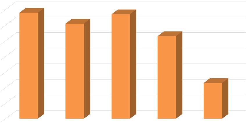
140 Original Data Phase 1 Augmented Data 140 2 Augmented Data
Phase Phase 3 Augmented Data
120 120
Data Volume
Data Volume 100 100
80 80
Phase 3 Phase 3
60 Phase 2 60
Phase 1 Phase 2
40 40
Phase 1
20 20
Knowledge Knowledge
0 0
Dim 1 Dim 2 Dim 3 Dim 4 … Dim N
Dimension Dim 1 Dim 2 Dim 3 Dim 4 … Dim N
Dimension
(a) Augmentation with searched static policies (b) Augmentation with random policies
Figure 4: An abstract view of augmentation on deficient data. The black bars shows the data distri-
bution of the original training data over the knowledge dimensions; while green, blue, yellow bars
stand for data generated from the 1st to 3rd phases of augmentation. The red dotted lines show
the data amount of the most deficient dimension upon completion of certain training phase with
augmentation.
Table 7: Details of the hyperparameters in our experiments: We used the models: Wide-ResNet (40-
2, 28-2, 28-10) (Zagoruyko & Komodakis, 2016), Shake-Shake (26 2x32d, 26 2x96d, 26 2x112d)
(Gastaldi, 2017), PyramidNet+ShakeDrop (Han et al., 2017; Yamada et al., 2019) and ResNet-50
(He et al., 2016).
Dataset Model Batchsize initial LR LR schedule weight decay
Wide-ResNet-40-2 256 0.1 cosin 2e-4
Wide-ResNet-28-10 256 0.1 cosin 5e-4
CIFAR-10 Shake-Shake(26 2x32d) 256 0.01 cosin 1e-3
Shake-Shake(26 2x96d) 256 0.01 cosin 1e-3
Shake-Shake(26 2x112d) 256 0.01 cosin 2e-3
PyramidNet+ShakeDrop 256 0.05 cosin 5e-5
Wide-ResNet-28-2 128 0.01 cosin 1e-3
Reduced CIFAR-10 Wide-ResNet-28-10 128 0.01 cosin 1e-3
Shake-Shake(26 2x96d) 128 0.2 cosin 1e-4
Wide-ResNet-40-2 256 0.1 cosin 2e-4
CIFAR-100 Wide-ResNet-28-10 256 0.1 cosin 5e-4
Shake-Shake(26 2x96d) 256 0.01 cosin 1e-3
SVHN Wide-ResNet-28-10 256 0.01 cosin 5e-4
ImageNet ResNet-50 512 0.05 step LR 1e-4
A.3 STANDARD BENCHMARK TRAINING DETAIL
CIFAR10/Reduced CIFAR10/CIFAR100/SVHN training details: For CIFAR10, we perform ex-
periments with the following models including Wide-ResNet-40-2, Wide-ResNet-28-10 (Zagoruyko
& Komodakis, 2016), Shake-Shake(26 2x32d), Shake-Shake(26 2x96d), Shake-Shake(26 2x112d),
and PyramidNet+ShakeDrop (Yamada et al., 2019). In addition, we evaluated our method on re-
duced CIFAR10 dataset which includes 4K training samples (randomly chosen) with Wide-ResNet-
28-2, Wide-ResNet-28-10 and Shake-Shake(26 2x96d) models. We experiment with cifar-100 on
Wide-ResNet-40-2, Wide-ResNet-28-10, Shake-Shake(26 2x96d), Shake-Shake(26 2x112d) and
PyramidNet+ShakeDrop. These are the same models used in the experiments conducted in Fast
AA. For SVHN dataset, we experiment with Wide-ResNet-28-10 on the core data of SVHN. Cosine
learning rate scheduler and mini-batch size of 256 are adopted in all of our experiments.
14Under review as a conference paper at ICLR 2021
As training epochs for various models are different, the complexity phases are defined respectively
according to individual models. For Wide-ResNet-40-2 and Wide-ResNet-28-10, three phases are
200, 30, and 20 epochs respectively. For Shake-Shake(26 2x32d), Shake-Shake(26 2x96d), Shake-
Shake(26 2x112d) and PyramidNet+ShakeDrop, three phases are 1800, 300, and 100 phases re-
spectively. For reduced CIFAR10, three phases are 450, 30, and 20 epochs for Wide-ResNet-28-2,
Wide-ResNet-28-10 models and 1500, 200, 100 epochs for Shake-Shake(26 2x96d) model.
ImageNet training details: For Imagenet, we conduct experiment with ResNet 50. The complexity
phases are 270, 30, 20 epochs respectively. We use step learning scheduler in the experiment to keep
consistent setting with Fast AA.
A.4 EXPERIMENTS ON N UMBER O F O PERATION
We explore the influence of different number of operations in a sub-policy on stochastic augmenta-
tion in this experiment. As shown in figure 5, when number of operations in a sub-policy is larger
than 3, the downgrade of performance is clear. Our interpretation is overlapped operations beyond
certain number may cause downgrade of image quality and in turn affect the augmentation perfor-
mance negatively.
97.50%
97.40%
80.00%
Test Accuracy
97.30%
Test Accuracy
79.00%
97.20%
78.00%
97.10%
77.00%
97.00%
76.00%
96.90%
75.00% 96.80%
1 2 3 4 5 1 2 3 4 5
Number Of Operations Number Of Operations
(a) Test Accuracy with WResNet-40-2 on CIFAR-100 (b) Test Accuracy with WResNet-28-10 on CIFAR-10
Figure 5: Influence of number of operations in a sub-policy on stochastic augmentation
A.5 MULTI-STAGE TRAINING LOSS PROFILE
Figure 6 shows the training loss profile for different epoch allocation of multi-stage augmentation.
____ ____ ____ train loss ____ train loss ____
____ ____
train loss
____ test loss ____ test loss
____ test loss
Loss
Loss
Loss
Epoch Epoch Epoch
(a) Three stage strategy with 50, 50, (b) Three stage strategy with 50, (c) Three stage strategy with 70, 70,
100 epochs allocated for stage 1, 2, 100, 50 epochs allocated for stage 1, 60 epochs allocated for stage 1, 2, 3
3 respectively 2, 3 respectively respectively
Figure 6: Training loss with various stage-epoch allocation strategy
15Under review as a conference paper at ICLR 2021
A.6 FACE RECOGNITION TRAINING DETAIL
We trained the system using MobileFaceNet (Chen et al., 2018) architecture with ArcFace loss
(Deng et al., 2018). Training backbone is adapted to Fast AA system and the training conducted
with the same settings described in Fast AA study apart from the search depth parameter which set
as 100. We adapt the learning rate of 0.1 with 512 batch size to speed up the training. We trained
the model for 50 epochs and learning rate is divided by 10 on epoch numbers 10,20 and 30.
3 stages training approach is done with 3 new additional augmentation methods. One of the addi-
tional operations is aging process which is based on StarGAN (Choi et al., 2017). In order to achieve
aging effect, StarGAN is trained on Cross-Age Celebrity Dataset(CACD) (Chen et al., 2014). This
dataset contains 160k images of 2000 celebrities with age ranges between 16 and 62. After aligning
the images in the dataset, age ranges are set as 10-20, 20-30, 30-40, 40-50, 50-99 and StarGAN
system is trained with these 5 classes by using default parameters. Subsequent to getting results,
all classes are selected except 10-20 age range as the potential augmenters. Other additional op-
eration is pose change and it is provided by employing (YadiraF). In order to achieve side faces, a
given face image is turned on the x-axis with the angles defined between -45 and 45 degrees. The
last of the additional operations is expression change. Expression change model is based on GAN-
imation (Pumarola et al., 2018). For expression change augmentation, each image from CASIA is
selected and augmented with 8 different (angry, disgusted, happy, sad, contemptous, fearful, neutral,
suprised) expressions.
In the first stage of training all of the operations including the additional ones are used for 14 epochs.
In the second stage, the additional complex augmenters turned off and training continued until 20th
epoch. In the last step, all of the augmenters turned off and the whole training is completed.
A.7 TEXT DETECTION TRAINING DETAIL
We trained our implementation of EAST (Zhou et al., 2017) architecture that uses PVANET (Kim
et al., 2016) as its backbone with ICDAR 2017 MLT dataset. In addition, this model is integrated
into Fast AA system and several experiments are performed with this system to provide comparative
results. ICDAR 2017 MLT dataset provides 7.2K images for training, 1.8K images for validation,
and 9K images for testing. The learning rate of 0.001 with cosine learning rate scheduler and mini-
batch size of 24 are adopted, and the same settings are used for all experiments that we conducted
for text detection task.
We also added 3 new geometry based (Distort, Stretch, Perspective) augmentations from (Luo et al.,
2020) and a color based (LocalGamma) augmentation to the default augmentation list while keeping
the baseline augmentations same with the original EAST (Zhou et al., 2017). These three geometry
based augmentations are applied only to the bounding box areas. It is good to inform about that
these additional augmentations are integrated to Fast AA system for comparing it with our method
in equal conditions.
3 separate models are trained for our experiments in text detection task and we evaluated them over
9K test images with the standard evaluation method for the text localization task of ICDAR MLT
2017 competition.
We trained a model with only applying the baseline augmentations. Another model is trained with
using the policies that are found by Fast AA system. For the last model that is trained by using
our approach, we applied 2 stages augmentation along training. In the first stage, the baseline
augmentations with 1.0 probability and the remaining augmentations including the additional ones
with 0.5 probability are applied for 160 epochs and the baseline augmentations are applied only for
the last 40 epochs.
It is also good to note that all models that we mentioned above are trained from the scratch without
using any pre-trained weights for total of 200 epochs.
E-Score: A fast and approximate metric for EAST RBOX text detector
To speed up both the training and the evaluation phases, a customized metric is used in our experi-
ments. This metric is faster to calculate and provides an approximate for F1 score. To give a further
explanation, EAST is evaluated over a dataset by F1-score given a fixed IOU threshold like the other
16You can also read