Improvements in Loss Given Default Forecasts for Bank Loans
←
→
Page content transcription
If your browser does not render page correctly, please read the page content below
Improvements in Loss Given Default Forecasts
                                      for Bank Loans

                                           Abstract
   An accurate forecast of the parameter loss given default (LGD) of loans plays a crucial role
for risk-based decision making by banks. We theoretically analyze problems arising when
forecasting LGDs of bank loans that lead to inconsistent estimates and a low predictive pow-
er. We present several improvements for LGD estimates, considering length-biased sampling,
different loan characteristics depending on the type of default end, and different information
sets according to the default status. We empirically demonstrate the capability of our pro-
posals based on a data set of 69,985 defaulted bank loans. Our results are not only important
for banks, but also for regulators, because neglecting these issues leads to a significant under-
estimation of capital requirements.

Keywords: Bank loans, Credit risk, Forecasting, Loss given default, Workout process

JEL classification: G21, G28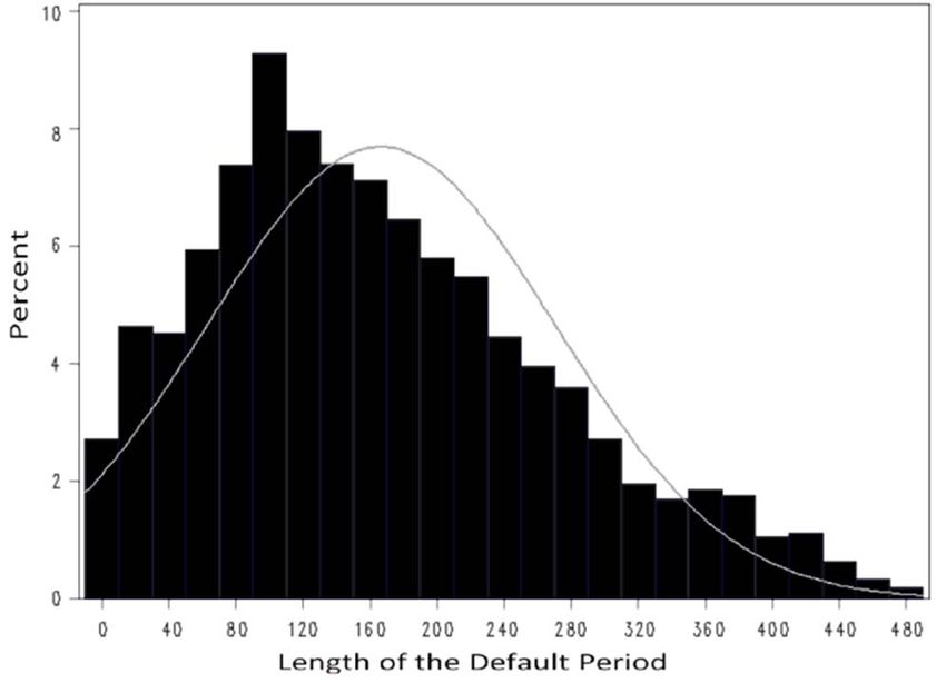
1    Introduction

    The most central risk parameters of a loan are the probability of default (PD) and the loss

given default (LGD). A decade ago, the focus of academic research and banking practice was

mainly on the prediction of PDs, but more recently, substantial effort has been put into model-

ing LGDs. One reason for this is the requirement of the Basel II / III framework for banks to

provide their own estimates of the LGD when using the advanced internal ratings-based (A-

IRB) approach for corporates or the IRB approach for retail exposures. In addition to the

regulatory requirement, accurate predictions of LGDs are important for risk-based decision

making, e.g. the risk-adjusted pricing of loans, economic capital calculations, and the pricing

of asset-backed securities or credit derivatives (cf. Jankowitsch et al., 2008). Consequently,

banks using LGD models with high predictive power can generate competitive advantages,

whereas weak predictions can lead to adverse selection.

    There are different streams of LGD-related literature. Some studies seek to estimate the

distribution of LGDs for credit portfolio modeling (cf. Renault and Scaillet, 2004; Calabrese

and Zenga, 2010), whereas others analyze the factors influencing individual LGDs. Further-

more, some studies deal with the relation between PDs and LGDs (cf. Frye, 2000; Altman et

al., 2005; Acharya et al., 2007; Bade et al., 2011). Although most of the literature consists of

empirical studies for corporate bonds, a smaller fraction focuses on bank loans, whether retail

or corporate, mainly due to limited data availability. A survey of empirical studies of LGDs

with a classification into bank and capital market data can be found in Grunert and Weber

(2009).

    For bank loans, the estimation of LGDs is usually based on discounted recovery cash

flows, leading to workout LGDs. A first step has been taken towards forecasting individual

LGDs for bank loans by empirical studies reporting LGDs for different categories of influence

factors (cf. Asarnow and Edwards, 1995; Felsovalyi and Hurt, 1998; Eales and Bosworth,

                                                1
1998; Araten et al., 2004; Franks et al., 2004). More recent studies analyze factors influencing
LGDs via linear regressions (cf. Citron et al., 2003; Caselli et al., 2008; Grunert and Weber,
2009), log regressions (cf. Caselli et al., 2008), or log-log regressions (cf. Dermine and Neto
de Carvalho, 2006; Bastos, 2010). Bellotti and Crook (2012) and Loterman et al. (2012) com-
pare the performance of different models constructed as combinations of different modeling
algorithms and different transformations of the recovery rate, e.g. OLS regressions or decision
trees, on the one hand, and log or probit transformations on the other hand. Bastos (2010)
proposes to model LGDs with nonparametric and nonlinear regression trees.
The main motivation of this paper is to improve forecasts of LGDs for bank loans. We the-
oretically analyze several problems that arise when forecasting LGDs and derive recommen-
dations for action in order to get consistent estimates with high predictive power. We apply
the proposed methods to a bank internal data set consisting of 69,985 defaulted loans of a
large German bank and analyze the improvements that can be achieved. We discuss our im-
provements within the typical steps of the modeling process. After all payments during the
workout processes have been collected for the modeling data set, which consists of historical
data of defaulted loans, the realized workout LGDs have to be calculated.1 Within the calcula-
tion of LGDs, we observe the effect that samples of historical LGDs are usually biased, due to
differences in the duration of the workout process. As the modeling data set usually consists
of defaults with completed workout process, defaults with a long workout process are un-
derrepresented because it is more likely that the workout process started before or will end
after the available observation period. However, defaults with a long workout process, on
average, have higher LGDs. Consequently, this underrepresentation of defaults with high
1
For retail loans, a default is usually assigned at a contract level. Conversely, for corporate loans, a default is
generally determined at a firm level, so that several contracts of a firm default simultaneously. This is in line
with the regulatory requirements, see Basel Committee on Banking Supervision (2005b), §455, and has to be
considered in the calculation of LGDs.
2LGDs leads to an underestimation of LGDs. To avoid the resulting underestimation of LGDs,
we propose a procedure for restricting the modeling data to get consistent LGD estimates
(Improvement 1).
Using calculated LGDs for the modeling data set, prediction models for LGDs can be de-
veloped to apply them to the scoring data set, which consists of new loans, non-defaulted ex-
isting loans, and defaulted existing loans. For new loans, LGD estimates are not only required
to determine the required capital backing, but also a high accuracy of individual LGD esti-
mates is essential to avoid adverse selection. In the literature, the prediction of individual
LGDs is mostly based on a direct regression on LGDs. However, the estimation of LGDs with
a single model often performs poorly. We discover that it is important to distinguish between
recovered loans and write-offs in the model design because the characteristics of both types of
default end can be very different. Against this background, we propose a two-step estimation
of LGDs that strongly outperforms the direct regression approach. In the first step, the proba-
bility of a recovery/write-off is estimated. In the second step, the LGDs of recovered loans, as
well as the LGDs of write-offs, are predicted separately. These predictions are combined into
the total LGD forecast (Improvement 2).
Furthermore, the existing literature on LGD modeling does not explicitly deal with LGDs
for defaulted loans, although for defaulted loans with an active default status, estimates of
LGDs are required, e.g. for regulatory and economic capital calculations. In this case, only the
portfolio LGD, and not the individual LGD, is of interest. However, if the average LGD of the
modeling data is assigned to the portfolio, the LGD is significantly underestimated. The rea-
son is that the information set of defaulted loans differs from the information set of non-
defaulted loans. For defaulted loans an estimator conditional on the specific default status of a
loan is required, whereas the average LGD is an unconditional estimator and leads to incon-
sistent LGD estimates. Against this background, we propose a consistent estimator for de-
faulted loans (Improvement 3).
3The proposed three improvements have a significant impact on LGD forecasts and should
be considered when modeling LGDs because neglecting these issues leads to a significant
underestimation and low accuracy of LGDs. However, to the best of our knowledge, no re-
search has addressed these issues as yet. The remainder of this paper is structured as follows.
Section 2 contains a theoretical derivation of the three Improvements. In Section 3, we present
an empirical study in which we analyze the extent of each improvement on the basis of real
data. Our conclusions are presented in Section 4.
2 Theoretical analysis of LGD forecasts
2.1 Calculation of workout LGDs
There are some relevant differences between LGDs of corporate bonds and bank loans.
First, LGDs of bank loans are typically lower than LGDs of corporate bonds. According to
Schuermann (2006), this empirical finding is mainly a result of the higher seniority of loans
(on average), and better monitoring. Second, LGDs of corporate bonds are typically deter-
mined on the basis of market values, resulting in “market LGDs”, whereas the LGDs of bank
loans are usually “workout LGDs”. If the market value of a bond directly after default is di-
vided by the exposure at default (EAD), which is the face value at the default event, we obtain
the market recovery rate (RR). Application of the equation LGD = 1 – RR results in the mar-
ket LGD. Conversely, the workout LGD is based on actual cash flows that are connected with
the defaulted debt position. These are mainly discounted recovery cash flows, but they are
also discounted costs of the workout process. If these cash flows are divided by the EAD, we
obtain the workout LGD. Even though the calculation of workout LGDs is more complex, the
advantage is that the results are more accurate and that this approach is applicable for all types
of debt (cf. Calabrese and Zenga, 2010).
4For the forecasting of LGDs, we have to calculate historical workout LGDs for our model-
ing data. Let S be a set of loans and i S , an individual loan. The workout LGD of loan i is
typically expressed as follows:2
RCFi Ci
LGDi 1 , (1)
EADi
where RCFi stands for the sum of discounted recovery cash flows of loan i, Ci represents
the sum of discounted direct and indirect costs of loan i, and EADi is the exposure at default
of loan i.3 Equation (1) leads to LGD = 0 if the recovery cash flow equals the exposure at de-
fault plus the costs of the workout process. In this context, it is important to notice that usually
only direct costs can be charged to the obligor whereas indirect costs have to be borne by the
bank.4 If the loan defaults completely, the LGD can even be higher than 1 if there are addi-
tional costs that arise during the workout process. However, a defaulted loan can have two
different types of default ends, which directly influence the calculation of LGDs: some con-
tracts can be recovered, whereas other contracts have to be written off.
Recoveries (RCs): In the case of a recovery, the default reason no longer exists, e.g.
the obligor paid the amount that was in arrears, or a new payment plan has been ar-
ranged. Thus, the contract is henceforth handled as a normal non-defaulted loan.
Write-offs (WOs): If the chance of recovering additional money from the obligor or
the realization of collateral is considered to be small, the contract will be written off.
Thus, there are generally no further payments for this contract.
2
Cf. Franks et al. (2004) or Calabrese and Zenga (2010).
3
We used the effective interest rate to discount the cash flows as this method has been favored by the nation-
al banking supervisor. For details regarding appropriate discount rates, see Basel Committee on Banking Super-
vision (2005a) and Maclachlan (2005).
4
A description of direct and indirect costs in context of calculating LGDs can be found in Franks et al.
(2004).
5While equation (1) is correct for write-offs, we also have to consider the exposure at recovery
(EARC) for the case of RCs. At the time of recovery, there is still a significant exposure re-
sulting from installments after the time of recovery. However, because the EARC reduces the
economic loss resulting from a default, but the EARC is not included in the cash flows, we
have to add the (discounted) exposure at recovery EARCi of loan i to the corresponding (dis-
counted) recovery cash flows:
RCFi Ci EARCi
LGDi 1 . (2)
EADi
Within the framework of the empirical study we apply equations (1) and (2) to calculate
LGDs of defaulted loans for a data set of a large German bank.
2.2 Length-biased sampling and restriction of the data set
Although the calculation of historical LGDs is rather unproblematic, the choice of an ade-
quate data set, which serves as a basis for LGD forecasts, is difficult. In this connection it
should be noted that banks are mainly interested in the total LGD of contracts, not just in the
loss in a predefined period after default (cf. Bastos, 2010). Thus, the modeling data of banks
usually consist of the historical defaults with completed workout processes. For example,
Grunert and Weber (2009) analyze recovery rates of loans that defaulted between 1992 and
2003. They note that only loans with completed workout processes are considered, leading to
a small number of defaults, as defined, in the years 2002 and 2003. Similarly, the calculated
LGDs of Asarnow and Edwards (1995) are based on all defaults between 1970 and 1993
where the workout process has been completed. However, if we develop LGD models on the
basis of all defaults that are available with a completed workout process, defaults with a short
workout process are overrepresented, due to interval censored data. This is illustrated in Fig-
ure 1.
6- Figure 1 about here -
Since LGDs and the duration of the workout process are not stochastically independent, both
the average duration of the workout process and also the average LGD are biased if this effect
is ignored. If we were solely interested in the duration of the workout process, we could ac-
count for censoring, e.g. by using the proportional hazard or accelerated lifetime model.5
However, we want to determine the LGDs of censored data, not the duration, so we cannot
apply these models. In Proposition 1, we show that the censored data lead to an underestima-
tion of LGDs. Furthermore, we propose how to restrict the data set in order to get unbiased
results.
Proposition 16
Let iS be a loan, i is the point in time of default of loan i, and Ti is the duration of the
i and of T , and the correla-
workout process for loan i.7 Assume i to be independent of LGD i
i ) between T and LGD
tion (Ti , LGD i to be positive. In addition, assume the existence of a
i
barrier Tmax, with Ti Tmax . Finally, and are two points in time with < and
Tmax . Then the following statements hold:8
(I) E LGD
i E LGD
i T .
i i i
5
The estimation of the survival function for censored data using nonparametric and parametric methods is
described in Kiefer (1988).
6
The proof of the proposition is presented in Appendix A.
7
Random variables are denoted by a tilde “~”.
8 i and T are conditionally independent for a
It may be argued that it is more reasonable to assume that LGD i
given realization of a macroeconomic factor. However, the results of part (I) and (II) remain valid if the corre-
sponding expressions are formulated conditional on the macroeconomic factor. To keep it concise, we present
the unconditional results.
7 i T , and LGD
i , LGD
(II) The random variables LGD i T T
i max max i i
are identically distributed, which implies
E LGD
i E LGD
i T
i max
i T T .
E LGD max i i
If we model LGDs on the basis of defaults with completed workout processes, the data set
consists of observations where the default occurs after the beginning of the observation peri-
od, i.e., i , and the point in time of the end of the default is i Ti . Thus, an estima-
tion of LGDs on the basis of the complete sample leads to an underestimation of LGDs due to
Proposition 1(I). The impact of this underestimation is greater when the time period that is
covered by the data of a bank is shorter. The relevance of this issue becomes apparent if we
look at the minimum data requirements for estimates of LGDs according to the Capital Re-
quirements Directive (2006/48/EC) of the European Union. According to the directive, LGD
estimates must be based on a data observation period of at least 5 years for corporate and 2
years for retail exposures if the bank uses its own estimates of LGDs for the first time. Subse-
quently, the minimum data observation period increases to 7 years and 5 years, respectively.
For these data observation periods, the problem of uncompleted defaults can lead to a signifi-
cant underestimation of LGDs.9
However, according to part (II) of the proposition there are two ways to circumvent this
problem. First, we can apply the condition i Tmax , which leads to a reduction of the
data set to loans with default begin between the beginning of the observation period and Tmax
before the end of the observation period. Second, we can apply the condition
Tmax i Ti , so that we restrict the data to loans with default end between Tmax after
9
Cf. Capital Requirements Directive (2006/48/EC), Appendix VII, Part 4, § 82 and § 86.
8the beginning of the observation period and the end of the observation period. In both cases,
the statement of part (II) of the proposition implies that the restriction of data results in unbi-
ased LGD estimates. Summarized, this leads to
Improvement 1: Constraining the modeling data set to prevent inconsistent LGD esti-
mates due to restricted data observation periods
In the empirical section 3.2 we show how to apply Proposition 1 to real data and we ana-
lyze to which extent the bias occurs if data is not restricted.
2.3 LGD forecasting for non-defaulted loans
Most of the empirical studies regarding factors influencing LGDs perform linear regres-
sions, and sometimes log or log-log-regressions, with the target variable LGD or RR. Howev-
er, only a few studies, like Caselli et al. (2008), Bastos (2010), or Belotti and Crook (2012),
report out-of-sample tests of the specified models.10 This is surprising, since it is essential for
banks that the models deliver a high accuracy of LGD estimates for unobserved data so that
they do not suffer from an adverse selection problem.11 To illustrate this, assume that there are
two equally sized groups of customers that are different with regard to their LGDs, whereas
all other characteristics, e.g. the PDs, are equal. Customers of group “good” have low LGDs
and customers of group “bad” have high LGDs. Let the fair interest rates be ig for group
“good”, ib for group “bad”, and ia for the average interest rate across all customers. Let bank
(I) not be able to distinguish the two groups, whereas, conversely, a competing bank (II) is
10
This is also noticed by Bastos (2010). Examples for empirical studies that focus on in-sample analyses are
Citron et al. (2003), Dermine and Neto de Carvalho (2006), Grunert and Weber (2009), and Loterman et al.
(2012).
11
The adverse selection problem was introduced in the literature by Akerlof (1970).
9able to differentiate between the two groups. As a consequence, bank (II) can attract more customers of group “good” because the bank can offer the lower interest rate ig
a set and x = ( x1 , ..., xk ) X be a vector of random borrower, loan, or collateral specific
characteristics. Consequently, a linear regression model with a dependent variable LGD that
does not consider the distinction between write-offs and recoveries can be expressed on the
basis of the set L { | : X linear function} of linear functions according to
x * ( x )+ ,
LGD (3)
*
where * : arg min( E (2 )) and stands for the respective random error term. This implies
L
that the expected LGD of a credit with specific characteristics x S can be estimated as
x = * ( x) .
E LGD
Since we have detected significant differences between the characteristics of recovered
loans and write-offs, it is reasonable to introduce a random variable x0 that is Bernoulli-
distributed with values WO (= write-off) and RC (= recovery). On this basis, we consider two
separate regressions, one for write-offs and one for recoveries:
( x , x WO ) * ( x ) +
LGD 0 WO WO , * , (4)
( x , x RC ) * ( x ) +
LGD 0 RC RC , * , (5)
where WO
*
: arg min( E (WO
2
, ))
and RC
*
: arg min( E (RC
2
, ))
.
L L
Consequently, the expected loss of a loan with specific characteristics x0 and x X that
has to be written-off can be estimated according to E LGD 0 WO
( x , x WO ) * ( x ) and the
expected loss of a recovered loan with specific characteristics x X corresponds to
E LGD 0 RC
( x , x RC ) * ( x ) .
x can be transformed
Using these estimations, the credit specific expected loss E LGD
according to:
11
E LGD WO
x * ( x ) P( x WO | x ) * ( x ) (1 P( x WO | x )) .
0 RC 0 (6)
Consequently, it remains to develop an estimator of the (conditional) write-off probability
P( x0 WO | x) E( I ( x0 WO) | x) , where I () denotes the indicator function. In this context,
we first define a function : X [0,1] such that, for all x X , the value ( x ) [0,1] is
interpreted as a credit specific score. If s [0,1] stands for a score threshold, a credit is as-
sumed to be a write-off (i.e., x0 WO ) if ( x ) s . Otherwise, i.e., if ( x ) s , the credit is
treated as a recovery (i.e., x0 RC ). On this basis, the estimation of the credit specific ex-
pected LGD corresponds to:
E LGD WO
x * ( x ) I ( ( x ) s) * ( x ) I ( ( x ) s) .
RC (7)
The accuracy of this estimation depends on the predictive accuracy of I ( ( x ) s ) and
( x ) , respectively. A standard tool for the assessment of the predictive accuracy of ( x ) is
the so-called receiver operating characteristic (ROC) curve.13 Within the framework of the
following proposition, we show that the higher the ROC curve, the higher the accuracy of
( x ) in the sense of a lower mean-squared error of estimation (7). Furthermore, we show
how to determine the weighted average of the right-hand side of (7) over different values of s
as it is possible that a specific score threshold s is not assumed to be appropriate.
Proposition 214
Consider score functions , 1 , 2 , and assume E( I ( x0 WO) | x) > 0. Furthermore, let
the following properties be fulfilled for all s1 , s2 [0,1] with P(1 ( x ) s1 | x0 RC )
P( 2 ( x ) s2 | x0 RC ) :
13
A detailed description of ROC curves can be found in Hosmer and Lemeshow (2000).
14
The proof of the proposition is presented in Appendix B.
12(a) P(1 ( x ) s1 | x0 WO) P( 2 ( x ) s2 | x0 WO) ,
* ( x )) 2 | ( x ) s , x ) E (( LGD
(b) E (( LGD * ( x )) 2 | ( x ) s , x ) , and
WO 1 1 0 WO 2 2 0
* ( x )) 2 | ( x ) s , x ) E (( LGD
(c) E (( LGD * ( x )) 2 | ( x ) s , x ) .
RC 1 1 0 RC 2 2 0
Then the following statements hold:
(I) For all s1 , s2 [0,1] with P(1 ( x) s1 | x0 RC ) P( 2 ( x) s2 | x0 RC ) we have
( * ( x ) I ( ( x ) s ) * ( x ) I ( ( x ) s ))2 )
E (( LGD WO 1 1 RC 1 1
E (( LGD ( ( x ) I ( ( x ) s ) ( x ) I ( ( x ) s ))2 ).
* *
WO 2 2 RC 2 2
(II) Let s be a random variable with values in [0, 1], and F the corresponding cumulative
distribution function with F(0) = 0. The (average) LGD estimation on the basis of an es-
timation procedure ( x ) and all “threshold scores” s can be determined as follows:
E (WO
*
( x ) I ( ( x ) s ) RC
*
( x ) I ( ( x ) s ) | x x )
WO
*
( x ) F ( ( x )) RC
*
( x ) (1 F ( ( x ))).
(III) If s is an equally distributed random variable with values in [0, 1], the (average) LGD
estimation of part (II) simplifies to:
E (WO
*
( x ) I ( ( x ) s ) RC
*
( x ) I ( ( x ) s ) | x x ) WO
*
( x ) ( x ) RC
*
( x ) (1 ( x )).
According to assumption (a), we consider score values 1 ( x) and 2 ( x) where the ROC
curve of 1 ( x) is always higher than the ROC curve of 2 ( x) . According to assumptions (b)
and (c), we only compare estimators that do not influence the estimation accuracy of condi-
tional LGD regressions (4) and (5), i.e., we only consider scores ( x ) that do not influence
the mean-squared error of (4) and (5). In part (I), we analyze the LGD estimation (7) and
show that the mean-squared error of the estimation approach (7) is lower if we apply “rating
procedure” 1 ( x) s than if we use procedure 2 ( x) s . Consequently, in order to achieve a
small mean-squared error it seems to be appropriate to apply a score function ( x ) with the
13highest possible ROC curve. Part (II) deals with the abovementioned problem of the adequacy
of a specific score threshold s . Against the background of part (II), it is possible to consider
all possible score thresholds s [0,1] and to assign a (probability) weight to each score
threshold in order to determine the “weighted mean estimator” of LGD. If each score thresh-
old s is assumed to be equiprobable, the resulting credit specific LGD estimator corresponds
to:
E LGD WO
x * ( x ) ( x ) * ( x ) (1 ( x ))
RC (8)
as shown in part (III). A comparison of (6) and (8) shows that the score value ( x ) can serve
as the desired estimator of P( x0 WO | x) . In this context, it should also be mentioned that,
for the standard regression (3), an estimator ( x ) is implicitly applied. This implicit estima-
tor immediately results from:
* ( x ) WO
*
( x ) ( x ) RC
*
( x ) (1 ( x ))
* ( x ) RC
*
( x) (9)
( x) * .
WO ( x ) RC ( x )
*
However, it may be worthwhile to apply an alternative estimator. Since the indicator variable
I ( x0 WO) | x is a binary dependent variable, we propose to apply a logit model according to
1
( x) , (10)
1 exp(ml* ( x ))
where ml
*
L is determined on the basis of the maximum likelihood method.15 Our method-
ology is related to the modeling approach of Bellotti and Crook (2012). They apply the fol-
lowing two-step approach. In the first step, it is determined whether LGD = 0, LGD = 1, or 0ever, in our setting, we do not model the final outcome of the LGD but the recovery/write-off
probability. Even if a recovery is often associated with very low outcomes of LGD, the events
that a loan can be recovered and the outcome LGD= 0 coincide only for a part of the data.
Moreover, we did not find different characteristics for defaults with LGD = 1. Consequently,
we get better results if the target variable is the type of default end (RC or WO). Summarized,
the aforementioned theoretical results lead to
Improvement 2: Explicit accounting for differences between write-offs and recovered
loans and application of a write-off probability estimator with a high ROC curve to
achieve a high predictive power in LGD forecasts
Again, the quantitative relevance of this improvement is analyzed on the basis of real data
in the empirical section 3.3.
2.4 LGD forecasting for defaulted loans
For defaulted loans, the state “default” and the EAD are realized, but the LGD is still a
random variable. Thus, for defaulted loans, LGD estimates are also required, e.g. for calcula-
tion of provisions, as well as economic and regulatory capital calculations. However, for this
purpose, no individual forecasts are required, but an estimate of the portfolio LGD can be
assigned to every single defaulted contract. In the empirical LGD literature, there is no com-
ment about differences between defaulted and non-defaulted loans that have to be considered
for this estimate. However, the portfolio LGD can be significantly underestimated if we use
the same model for both defaulted and non-defaulted loans. This finding also holds if we as-
sign the historical average LGD, which is the average LGD of the modeling data, to the port-
folio of defaulted loans. This is because we have different information sets for defaulted and
non-defaulted loans. In the modeling data, the LGDs are not conditional on the length of the
15workout process T, which has been shown in Proposition 1(II). However, for defaulted data,
we have additional information on the current length of the workout process t. Thus, we al-
ready know that T>t, so that we have to assign the LGD conditional on T>t. Because LGDs of
contracts with long workout processes are typically much larger than LGDs for short workout
processes, this leads to an underestimation of LGDs. This effect mainly stems from the differ-
ent average lengths of workout processes for loans that can be recovered and loans that have
to be written off.17 In Proposition 3(I), we show that ignoring the difference between the in-
formation sets would lead to a significant underestimation of the LGD, whereas in Proposition
3(II), we present a consistent estimator using the information on the current default length.
Proposition 318
Let the assumptions of Proposition 1 be fulfilled. Furthermore, consider a sequence of
j I (T t ))
loans denoted by j = 1, 2, …, where ( LGD j j is a sequence of independently and
identically distributed random variables, with each member of the sequence having expecta-
i I (T t )) . Furthermore, ( I (T t ))
tion value E ( LGD i j j is a sequence of independently and
identically distributed random variables, with each member of the sequence having expecta-
tion value E ( I (Ti t )) . Finally, the corresponding exposures at default EAD1, EAD2, … are
assumed to be deterministic and to fulfill the following conditions:
N j I {T t})
Var ( LGD Var ( I {Tj t})
(a) EAD j , (b), j
2
, and (c) 2
.
N
j j 1 j
EADk
j 1 j 1
EADk
k 1 k 1
Then the following statements hold:
i(model) ) E ( LGD
(I) E ( LGD i | T 0) E ( LGD
i | T t ).
i i
17
Details will be presented in section 3.2.
18
The proof of the proposition is presented in Appendix C.
16N
EAD j
j I {T t}
LGD j
(II) j 1
N
a.s.
N
i | T t .
E LGD i
EAD j I{Tj t}
j 1
Thus, for the modeling data, we can calculate the (EAD-weighted) average LGDs for all
contracts with T>t. If we proceed in this way for every value of t[0, Tmax], we can assign
LGDs to every defaulted loan using the information of the current length of the workout pro-
cess, and, as shown in Proposition 3(II), we get consistent LGDs when we apply the model.
Since these LGDs are calculated on the basis of modeling data with a minimum default length
(MDL) of t, we call the corresponding values LGD(MDL = t). Summarized, the statements of
Proposition 3 lead to
Improvement 3: Accounting for the minimum default length of defaulted loans to
achieve consistent LGD forecasts
In the following chapter we empirically examine the relevance of the three improvements
on the basis of real data.
3 Empirical analysis of LGD forecasts
3.1 Description of the data set
The data set consists of 69,985 retail loans of a large German bank, where the end of the
workout process is between October 1, 2006, and September 30, 2008.19 The loans correspond
to several sub-portfolios of the bank, which can be divided into private and commercial loans
19
While most studies on LGDs present the number of loans that defaulted in a given period (the beginning of
the workout process), we focus on the end of the workout process. For details see sections 2.2 and 3.2..
17meeting the criteria of retail portfolios,20 as well as secured and unsecured loans. The descrip-
tion of the data set can be found in Tables 1, 2, and 3.
- Table 1 about here -
- Table 2 about here -
- Table 3 about here -
As can be seen in Table 1, the major part of the data consists of secured loans to private cli-
ents. As expected, secured loans on average have significantly lower LGDs than unsecured
loans, which is demonstrated in Table 2. Moreover we find that LGDs of private loans are on
average slightly lower than LGDs of commercial loans. In Table 3, we present additional
summary statistics for selected variables of private and commercial secured loans. For both
subportfolios, we present the number of previous defaults of the contracts, the default reasons,
and the types of default end. Default reasons that are applied in the bank are that the obligor is
past due for more than 90 days, a notice of cancellation, a court order, and a significant
downgrading.21 However, the default reason “court order” is not relevant for secured loans
because a notice of cancellation has to be sent before. In addition, we present the distribution
of occupational categories and marital status for private loans, whereas the limited or unlim-
ited liability is only relevant for commercial loans. The average collateralization level, de-
fined as the proportion between value of collateral and EAD, is 1.42 for private secured loans,
meaning that at the time of default the loans are overcollateralized on average. However, the
20
See, e.g., Basel Committee on Banking Supervision (2005b), §70.
21
The regulatory definition of default is similar but a bit vaguer. In addition to being past due for more than
90 days, a default is considered to have occurred if the obligor is unlikely to pay its credit obligations in full; see
Basel Committee on Banking Supervision (2005b), §452. However, some indications of unlikeliness to pay are
specified in §453, which include that the bank has filed for the obligor’s bankruptcy or a similar order or that
there is a significant perceived decline in credit quality.
18median is only 0.73, which illustrates that the major share of loans is not overcollateralized.
For commercial loans the collateralization level is significantly lower with on average 0.41.
The ratio “EAD/loan amount” is similar for private and commercial loans, with 0.67 and 0.73,
respectively. In addition, statistics about value of collateral, net loan amount, EAD, down
payment/EAD, and length of the default processes are shown in Table 3. Furthermore, for
private loans, we present statistics about annual income and the ration “loan amount/annual
income” in Table 3.
Subsequently, we analyze the largest subportfolio of secured loans to private clients with a
total of 59,442 contracts in more detail. The corresponding LGD frequency distribution is
presented in Figure 2.
- Figure 2 about here -
In the empirical literature about LGDs, it is often reported that the distribution of LGDs is
bimodal, with most LGDs being quite low (20%-30%) or quite high (70%-80%) (cf. Schuer-
mann, 2006). Although this seems to be true for corporate bonds, or the combined data for
corporate bonds and corporate loans, the distribution for retail loans can be quite different.
For our data covering secured loans to private clients, it is striking that the major share of
loans has a LGD that is close to zero, whereas a smaller share of loans is concentrated at val-
ues around 50%, and a small peak can be found for an LGD of 100%. This distribution has
similarities to the data set of Bastos (2010), who finds that about 55% of the loans have an
LGD close to zero and about 15% have an LGD close to one.22 However, in our data, the frac-
tion of LGDs close to zero is considerably higher, whereas the fraction of LGDs close to one
22
Moreover, a small peak can be observed at LGD between 40% and 50%.
19is substantially lower.23 The LGD distributions of the other sub-portfolios show some minor
differences to Figure 2. For secured loans of commercial clients, the distribution is very simi-
lar, but the small peak at LGD = 1 is missing. This might be a result of greater efforts being
made to recover a part of the exposure in connection with a better cost-benefit ratio due to
higher loan amounts. If the loans are unsecured, the LGDs are, on average, significantly high-
er for both private and commercial clients. However, for all sub-portfolios, there is a large
number of contracts with LGDs close to zero. Although the observations mainly consist of
loans that have been recovered, observations with high LGDs largely relate to contracts that
had to be written off. The distribution of LGDs for both types of default end (RC and WO) are
illustrated in Figure 3. It may be astonishing that in a few cases even for recovered loans very
high values of LGD can be obtained. In this connection it should be considered that indirect
costs are not charged to the obligor. Consequently, even for “full” recoveries, the resulting
LGD can be higher than zero. If the EAD is very low, the resulting LGD can reach these high
values.
- Figure 3 about here -
3.2 Length-biased sampling and restriction of the data set
Because the main driver of Improvement 1 is the positive relationship between LGD and
i ) for our data
the duration of the workout process, we first calculate the correlation (Ti , LGD
set. This correlation equals 0.2634, which confirms that LGDs are significantly larger for de-
faults with long workout processes. To examine this effect further, we next present the dura-
tion of the workout process separately for recovered loans and write-offs in our data set. As
23
In our data approximately 77 % of the loans have an LGD lower than 0.05 and 2 % of the loans have an
LGD between 0.95 and 1.05.
20can be seen in Figure 4, the workout process is typically significantly shorter for loans that
can be recovered than for write-offs. Since recoveries usually have significantly smaller
LGDs than write-offs, as already demonstrated in Figure 3, we have an essential reason for
the finding that defaults with a short workout process typically have small LGDs.
- Figure 4 about here -
As can also be seen in Figure 4, almost all workout processes for the presented data are
completed after 450 days. Hence, we set Tmax = 450 and restrict the data set according to
Proposition 1(II). As already noted, to restrict the data set we can apply condition
i Tmax or condition Tmax i Ti . In both cases, we ensure that the potential
observation period is at least 450 days for each loan, so that short spells are not overrepresent-
ed in the sample. We use the second of the mentioned alternatives because in this case we
consider the most recent defaults and ignore defaults from the beginning of the observation
period. Since our observation period comprises the time period between ( =) July 1, 2005,
and ( =) September 30, 2008, we restrict the analysis to loans with default ends between
( 450 =) September 24, 2006, and September 30, 2008. As a consequence of this re-
striction, the relative increase in LGD is 8.3%. Thus, LGDs would have been underestimated
by 8.3 % if the modeling data were not constrained. This in turn underlines the high relevance
of Improvement 1.
3.3 LGD forecasting for non-defaulted loans
3.3.1 Measurement of the predictive power of the model
The predictive power of the model can be evaluated at different stages. First, we evaluate
the performance of the logit-model ( x ) (see equation (10)) on the basis of the receiver oper-
21ating characteristic (ROC). Second, the linear models WO
*
( x ) and RC
*
( x ) (see regressions
(4) and (5)) are evaluated using the coefficient of determination R2. Finally, in order to assess
the total performance of the model, we combine the predictions of the two-step model accord-
ing to WO
*
( x ) ( x ) RC
*
( x ) (1 ( x )) (see part (III) of Proposition 2), and additionally
compute R2 for the combined forecast. However, the statistic expressing the predictive power
can be overestimated when it is calculated in-sample. Against this background, we evaluate
2
the models on the basis of the out-of-sample statistic. The out-of-sample statistic ROS , which
is proposed by Campbell/Thompson (2008), is computed as:
LGD LGD
M 2
i
i
2
ROS 1 i 1
, (11)
LGD LGD
M 2
i IS
i 1
i (with i = 1, …, M) are the
where LGD IS is the average LGD of the in-sample data, LGD
forecasted LGDs calculated out-of-sample (applying the model that is based on the in-sample
data), and LGDi are the realized LGDs of the out-of-sample data. This statistic measures the
reduction of the mean-square prediction error relative to the average LGD of the in-sample
2
data. The out-of-sample statistic is restricted to ROS 1 . If ROS
2
0 ( ROS
2
0 ), the forecasts
are better (worse) than the in-sample average.
3.3.2 Comparison of the two-step model and the direct regression by simulation
Since it is not obvious whether the implicit estimation procedure (9) or the logit model (10)
leads to a higher ROC curve, it is not clear if the two-step model is superior to a direct LGD
regression. Against this background, we test the corresponding hypothesis by an extensive
simulation study.
22Hypothesis
2
The out-of-sample coefficient of determination ROS, two-step of the two-step model (part (III) of
2
Proposition 2, together with (4), (5) and (10)), is higher than ROS, direct of a direct LGD regres-
sion (3).
Test of the Hypothesis by simulation
We analyze the performance of the proposed two-step model in comparison to a direct regres-
sion on LGDs on the basis of a simulation study. First, we simulate LGDs for a portfolio of
1,000 defaulted loans. When generating LGDs, we use a structure that incorporates differ-
ences between write-offs and recovered loans, consistent with our argument and empirical
findings. However, we choose a model structure that differs from equation (4) and from part
(III) of Proposition 2 to induce some model error.24 To generate the event of a write-off we
apply a factor model that is frequently used to generate default events.25 The advantage of a
factor model lies in the possibility to consider several observable and unobservable influenc-
ing factors. To be more specific, we identify the event of a write-off with the fulfillment of the
following inequality:
I ( x0 WO ) 1:
x21,1 x1 x22 x2 1 x21,1 x22 , (12)
with observable and unobservable factors x1 , x2 , (0,1) , a write-off barrier , and Ф as
the standard normal CDF. Because the argument of Ф is standard normally distributed, the
result () is uniformly distributed with () (0,1) . In our simulation, we set δ=0.8, lead-
ing to a 20% probability of a write-off. Similarly, we generate the LGDs within the group of
write-offs by:
24
We have also implemented different settings, but the basic results remain unchanged.
25
See e.g. Hull (2009), p. 515.
23 WO
LGD
x21,2 x1 x23 x3 1 x21,2 x23 , (13)
with x1 , x3 , (0,1) . Thus, the LGD is bound between zero and one. Altogether, the out-
come of LGD is calculated as:
I ( x 1) LGD
LGD WO , (14)
0
which implies that the LGD of recoveries is set to zero, since the variation of LGDs is usually
small for recovered loans.
According to our argument above, the event of a write-off and the LGD within the group
of write-offs can be influenced by different variables. However, some variables can be rele-
vant for both equations. Against this background, x1 influences both dependent variables, but
the coefficients can be different. Conversely, x2 and x3 each affect only one of the dependent
variables. Moreover, we assume that x1 , x2 , x3 are observable, whereas and are unob-
servable random variables. Thus, only x1 , x2 , and x3 are input variables for the regressions
that are subsequently applied.
In order to compare the performance of both modeling approaches, we perform a direct re-
gression, with the target variable LGD on the one hand, and apply the two-step model, on the
other hand. As stated above, we obtain the (total) LGD forecast of the two-step model as a
combination of different estimates according to part (III) of Proposition 2. After applying both
modeling approaches, we compare the out-of-sample R2 of the resulting LGDs with formula
(11). For the out-of-sample analysis, we generate 10,000 additional LGDs using formulas
(12)-(14).26
26
Due to the known LGD generating process, we can create an arbitrary number of LGDs for testing the
models out-of-sample. With an increasing number of LGDs, the measured predictive power converges towards
the true value.
24The simulation procedure above is performed for a broad range of parameter combinations.
The coefficients x21,1 and x21,2 are independently set to (0.1, 0.2, …, 0.9) and the coefficients
x22 and x23 are set to (0.1, …, 1– x21,1 ) and (0.1, …, 1– x21,2 ), respectively. This leads to a
total number of 2,025 different parameter combinations. For each parameter combination, we
repeat the simulation procedure 1,000 times and compare the average in- and out-of-sample
R2 of both models. The mean ROS,two-step
2
of the combined LGD estimates from the two-step
2
model is 0.599, whereas the mean ROS,direct of the direct regression is only 0.345 (cf. Table 4).
Moreover, the difference ROS
2
ROS,
2
two-step ROS, direct is positive for each individual parameter
2
combination, which confirms our hypothesis. Thus, the two-step model impressively outper-
forms the direct regression.
- Table 4 about here -
The application of our two-step approach to real data is presented in the following subsection.
3.3.3 Application of the two-step model to empirical data
The models for estimating LGDs are developed using SAS® Enterprise Miner. The models
for forecasting the write-off probabilities are estimated using multivariate logit-regressions
according to (10). We split the data into 70% training data (in-sample) and 30% validation
data (out-of-sample).27 For many of the categorical variables used, we achieved an improved
out-of-sample performance by aggregating the variables to a smaller number of classes, e.g.
27
Because the data base is sufficiently large, we do not use a k-fold cross-validation like Bellotti and Crook
(2012) or Bastos (2010).
25by using the variables “limited liability” or “unlimited liability” for commercial loans, instead
of the concrete legal form of a company. The predictive power of the different logit-models is
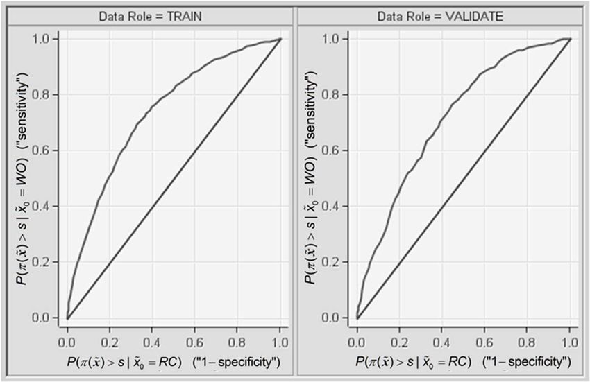
mainly evaluated on the basis of the ROC.28 In Figure 5, we present the ROC curves for the
largest sub-portfolio, which consists of secured loans to private clients. The value for the area
under the ROC curve for the training data is AUCIS 0.735 ; the respective value for the vali-
dation data is AUCOS 0.713 . As a final step, the coefficients of the model are calibrated on
the basis of the full data set, leading to an AUC value of AUCAll 0.730 . The explanatory
variables that are used in the model can be divided into borrower characteristics (e.g. the oc-
cupational category and the marital status; an important influencing factor for the sub-
portfolio of commercial loans is the liability of a company), collateral characteristics (e.g. the
type of collateral), and loan characteristics (e.g. the previous number of defaults).29
- Figure 5 about here -
Similarly, we develop the linear regression models for estimating LGDs in the scenario of
a write-off. Thus, we split the data set of contracts that had to be written-off into training and
validation data, and perform multivariate linear regressions. The predictive power of the vali-
2
dation data is evaluated with the coefficient of determination ROS,WO by applying formula
(11). For secured loans to private customers, the coefficients of determination for the selected
28
Interestingly, when checking the economical plausibility, i.e. the concordance with the working hypothe-
ses, the ROC curves for the training and the validation data generally become more similar if variables with
implausible coefficients are dropped, resulting in a reduced performance for the training data but an increased
predictive power for the validation data.
29
The publication of the concrete models, including the coefficients, is prohibited by the bank that provided
the data set of defaulted bank loans.
262
model are RIS,WO 0.199 and ROS,WO
2
0.176 .30 The final coefficients are calibrated on the
2
complete data set leading to RAll,WO 0.193 . Again, the relevant explanatory variables can be
classified into borrower characteristics (e.g. the occupational category), collateral characteris-
tics (e.g. the type and value of collateral), and loan characteristics (e.g. 1/EAD and down
payment/EAD). Similarly, we perform linear regressions for recovered loans. However, since
the LGDs of recovered loans mostly have only small variations, and these variations could not
be predicted accurately, we assign the historical average LGD for this type of default end.
After combining the model forecasts to get the total LGD estimate according to part (III) of
Proposition 2, we calculate the total R2 of the two-step model. The resulting values for the
two-step 0.189 and ROS, two-step 0.181 . Con-
2 2
training data and for the validation data are RIS,
versely, if we apply the direct regression approach to the same data set, we get
direct 0.044 and ROS, direct 0.042 . Thus, the proposed two-step model empirically strong-
2 2
RIS,
ly outperforms the direct regression approach.
Summarized, in view of the empirical results and the results of the simulation study we ob-
serve that consideration of Improvement 2 leads to a significantly higher predictive power in
comparison to the direct regression approach.
3.4 LGD forecasting for defaulted loans
According to Proposition 3(I) we should consider additional information about the current
length of the workout process because neglecting this information leads to an underestimation
of LGD. Furthermore, due to Proposition 3(II), the conditional expected value of the LGD
given a length t of the workout process can be estimated by
30 i (1 LGD
After transforming the LGD estimates using Loss ) EAD , it is also possible to evaluate the
i i
predictive power with respect to absolute instead of relative losses. This leads to coefficients of determination of
0.522 and 0.573, respectively.
27N
EAD j LGD j I (T j t )
Default,i : LGD MDL t ,
j 1
LGD N
(15)
EAD
j 1
j I (T j t )
where N and each j {1, ..., N} stands for a contract of the modeling data. The resulting
values of LGDs for the sub-portfolio of secured loans to private clients are presented in Figure
6. The unconditional LGD is about 21%. Strikingly, for contracts with a rather short MDL,
the average LGD increases, which coincides with our expectation. However, for contracts
with an MDL of more than 150 days, the average LGD decreases. Moreover, at MDL = 1
year, the LGD jumps about 9%.
- Figure 6 about here -
In order to obtain reliable forecasts of LGDs for defaulted loans, we analyze these findings
further. For this purpose, we examine which additional factors are most important for explain-
ing the variation in LGDs for defaulted loans. In addition to the information that is available
for non-defaulted loans, we know the default reason, which could be relevant for explaining
differences in LGDs. As already mentioned in section 3.1, the default reasons that are applied
in the bank are
(1) the obligor is past due for more than 90 days,
(2) a notice of cancellation or a court order, or
(3) a significant downgrading.
We find that the average LGD varies significantly depending on different default reasons. For
example, defaults with default reason 1 (being past due), on average, produce smaller losses
than defaults with default reason 2 (notice of cancellation or a court order).
28In order to analyze which explanatory variables are most relevant, we use regression trees
with the software SAS® Enterprise Miner.31 Regression trees are nonlinear and nonparametric
predictive modeling tools that split the data into several groups on the basis of a series of bi-
nary questions, e.g. “default reason = 1?” and “default period > 100 days?”. These questions
are set in a way that the information about the LGD is maximized.32 As noted by Bastos
(2010), regression trees are well-suited to producing accurate results of LGD forecasts using
only a few important explanatory variables. For different sub-portfolios, we find that the most
important explanatory variables are: (I) the abovementioned default reasons, (II) the duration
of the workout process, and (III) segmentation variables regarding the type of obligor (private
or commercial loans), and the type of collateral (secured or unsecured).
Since we want to include these additional influencing factors, we first partition our model-
ing data into classes that are homogeneous in terms of the default reason and the segmentation
variables, then we calculate LGD(MDL = t) for every class. Thus, we apply the estimator of
equation (15) for all contracts in our modeling data within one of these classes. In Figure 7,
we present the empirical LGDs for the largest sub-portfolio of secured loans to private clients,
separated by the default reason.
- Figure 7 about here -
There are some characteristics of the illustrations worth mentioning. First, for most contracts
with default reason 1, 2, or 3, the LGD increases with the default length, which is in line with
our expectation. Second, the average LGD of contracts with default reason 3 decreases for
small values of MDL and has a jump at MDL = 365 days. To understand this effect, we have
31
The first published study that models LGDs with regression trees was Bastos (2010). However, we apply
regression trees to forecast LGDs of defaulted instead of non-defaulted loans.
32
For details, see Breiman (1984).
29to consider that default reason 3 means a significant downgrading. Banks often retrieve addi-
tional scoring information from credit agencies. In the presented case, the bank updates the
values of the negative scoring characteristics one year after default. Thus, the negative scoring
could have already been changed during this period; however, the scoring information is cost-
ly, leading to non-frequent updates. If the negative scoring characteristic no longer exists at
this time, and if this is the only active default reason, a loan recovers, leading to a small LGD.
This effect was already visible in Figure 4, where we could observe a small peak of recovered
loans for a length of the workout process of 365 days. However, if default reason 3 still exists,
the probability of a write-off is quite high. Thus, the LGD jumps at a minimum default length
of one year. Summing up, these additional findings are the rationale behind the characteristics
of Figure 6 that has been presented earlier.
Next, we quantify for our data set whether the consideration of Proposition 3 has a material
impact. For this purpose, we choose to simulate the situation where we have to assign LGDs
to defaulted scoring data on January 2, 2007. Thus, our sample has to fulfill the following two
requirements - the contract defaulted before January 2, 2007, and the workout process ended
after January 2, 2007. We choose this date because we already know the realized LGDs of
these contracts, so we can contrast the estimates to the true values. If we ignored the addition-
al information about the current length of the workout process, we would assign the historical
average LGD of the sub-portfolio, which is 21.1%. However, due to Proposition 3(II), we
assign the LGDs that are presented in Figure 7. The resulting estimate of the portfolio LGD is
30.2%, which is materially higher than the historical average. The true average LGD, which
can be calculated when all workout processes have ended, is 29.4%. This shows that our LGD
estimator delivers reliable forecasts for defaulted scoring data. However, ignoring the updated
information regarding the minimum default length results in a significant underestimation of
LGDs. Against this background, the presented empirical results point out the high relevance
of Improvement 3.
304 Conclusion
In this paper, we identify several problems in modeling workout LGDs that can lead to in-
accurate LGD forecasts, and we propose methods for how to deal with these problems in or-
der to improve LGD forecasts. We apply these methods to a data set of 69,985 defaulted loans
of a large German bank. First, the LGDs within the modeling data can be significantly biased
downwards if all available defaults with completed workout processes are considered. This is
mainly due to length-biased sampling in connection with different lengths of the workout pro-
cesses for recovered loans and write-offs. We show how the modeling data could be restricted
in order to obtain unbiased LGD estimates. Second, we propose a two-step approach for mod-
eling LGDs of non-defaulted loans, from which different influencing factors of recoveries and
write-offs can be considered. We demonstrate the potential of this approach on the basis of a
simulation study. Furthermore, we demonstrate empirically that the predictive power is signif-
icantly improved in comparison to a direct regression approach. Third, we show that the LGD
for a portfolio of defaulted loans is biased if the prediction is based on regression models, or
historical averages, if the information set relating to the specific default status of a loan is ig-
nored. We propose a model for defaulted loans that estimates the portfolio LGD consistently.
Although all of these issues are relevant from an economic point of view, the first and third
improvements are also relevant for regulators, as a neglect of the presented problems leads to
an underestimation of LGDs and therefore to an undercapitalization of banks.
31References
Acharya, V.V., Bharath, S.T., Srinivasan, A., 2007. Does industry wide distress affect de-
faulted firms? Evidence from creditor recoveries. Journal of Financial Economics 85,
787–821.
Akerlof, G.A., 1970. The Market for 'Lemons': Quality Uncertainty and the Market Mecha-
nism. Quarterly Journal of Economics 84, 488–500.
Altman, E.I., Brady, B., Resti, A., Sironi, A., 2005. The link between default and recovery
rates: theory, empirical evidence, and implications. Journal of Business 78, 2203–2228.
Araten, M., Jacobs Jr., M., Varshney, P., 2004. Measuring LGD on commercial loans: An 18-
year internal study. The RMA Journal 4, 96–103.
Asarnow, E., Edwards, D., 1995. Measuring loss on defaulted bank loans. A 24-year-study.
Journal of Commercial Lending 77(7), 11–23.
Bade, B., Rösch, D., Scheule, H., 2011. Default and recovery risk dependencies in a simple
credit risk model. European Financial Management 17, 120–144.
Basel Committee on Banking Supervision, 2005a. Guidance on paragraph 468 of the frame-
work document, Bank for International Settlements.
Basel Committee on Banking Supervision, 2005b. International convergence of capital meas-
urement and capital standards – a revised framework, Bank for International Settlements.
Bastos, J.A., 2010. Forecasting bank loans loss-given-default. Journal of Banking and Finance
34, 2510–2517.
Bellotti, T., Crook, J., 2012. Loss given default models incorporating macroeconomic varia-
bles for credit cards. International Journal of Forecasting 28, 171–182.
Breiman, L., Friedman, J.H., Olshen, R.A., Stone, C.J., 1984. Classification and regression
trees. Wadsworth: Belmont, CA.
Calabrese, R., Zenga, M., 2010. Bank loan recovery rates: measuring and nonparametric den-
sity estimation. Journal of Banking and Finance 34, 903–911.
Campbell, J.Y., Thompson, S.B., 2008. Predicting excess stock returns out of sample: can
anything beat the historical average? Review of Financial Studies 21, 1509–1531.
Caselli, S., Gatti, S., Querci, F., 2008. The sensitivity of the loss given default rate to system-
atic risk: new empirical evidence on bank loans. Journal of Financial Services Research
34, 1–34.
Citron, D., Wright, M., Ball, R., Rippington, F., 2003. Secured creditor recovery rates from
management buy-outs in distress. European Financial Management 9, 141–161.
Dermine, J., Neto de Carvalho, C., 2006. Bank loan losses-given-default: a case study. Journal
of Banking and Finance 30, 1243–1291.
Eales, R., Bosworth, E., 1998. Severity of loss in the event of default in small business and
larger consumer loans. The Journal of Lending and Credit Risk Management, 58–65.
32You can also read