A Pseudo-SBAS Method To Invert 2D Deformations of The 2021 Central Greece Earthquake Sequence Using Multi-Track And Multi-Temporal Sentinel-1 SAR Data
←
→
Page content transcription
If your browser does not render page correctly, please read the page content below
A Pseudo-SBAS Method To Invert 2D Deformations of The 2021 Central Greece Earthquake Sequence Using Multi-Track And Multi-Temporal Sentinel-1 SAR Data Zhangfeng Ma ( jspcmazhangfeng@hhu.edu.cn ) Hohai University https://orcid.org/0000-0003-0044-7710 Xiaojie Liu Chang'an University Qihuan Huang Hohai University Guihua Li Hohai University Jihong Liu Central South University Cheng Zhou Sinopec Geophysical Research Institute Jia Hu Hohai University Zhuang Gao Hohai University Pengcheng Sha Hohai University Yan Cui Hohai University Shuhong Qin Hohai University Teng Huang Hohai University Jiandong Gao Hohai University Research Article
Keywords: Co-seismic Deformation, SAR interferometry (InSAR), Compressed Sensing, Strain Model, Small Baseline (SBAS), Central Greece Earthquake Sequence DOI: https://doi.org/10.21203/rs.3.rs-819348/v1 License: This work is licensed under a Creative Commons Attribution 4.0 International License. Read Full License
Submitted to Journal of Geodesy

 1   A Pseudo-SBAS Method to Invert 2D Deformations of the 2021 Central Greece

 2   Earthquake Sequence using Multi-track and Multi-temporal Sentinel-1 SAR Data

 3   Zhangfeng Ma1,2, Xiaojie Liu3,4, Qihuan Huang1, Guihua Li1, Jihong Liu5, Cheng Zhou6,

 4   Jia Hu1,7, Zhuang Gao1, Pengcheng Sha1, Yan Cui1, Shuhong Qin1, Teng Huang1, Jiandong

 5   Gao1,8

     1
 6       School of Earth Sciences and Engineering, Hohai University, Nanjing 211100, Jiangsu, P.R.

 7   China

     2
 8       Asian School of the Environment, Nanyang Technological University, Singapore 639798

     3
 9       School of Geological Engineering and Geomatics, Chang'an University, Xi'an 710054, Shaanxi

10       P.R. China

     4
11       Department of Civil Engineering, University of Alicante, Spain 03690.

     5
12       School of Geosciences and Info-Physics, Central South University, Changsha 410083, Hunan,

13       P.R. China

     6
14       SINOPEC Geophysical Research Institute, Nanjing 211103, Jiangsu, P.R. China

     7
15       Department of Geological and Atmospheric Sciences, Iowa State University, IA 50011, USA

     8
16       Jiangsu Province Surveying and Mapping Engineering Institute, Nanjing 210013, Jiangsu, P.R.

17       China

18   Corresponding author: (Qihuan Huang, InSAR@hhu.edu.cn)

19

20

                                                       1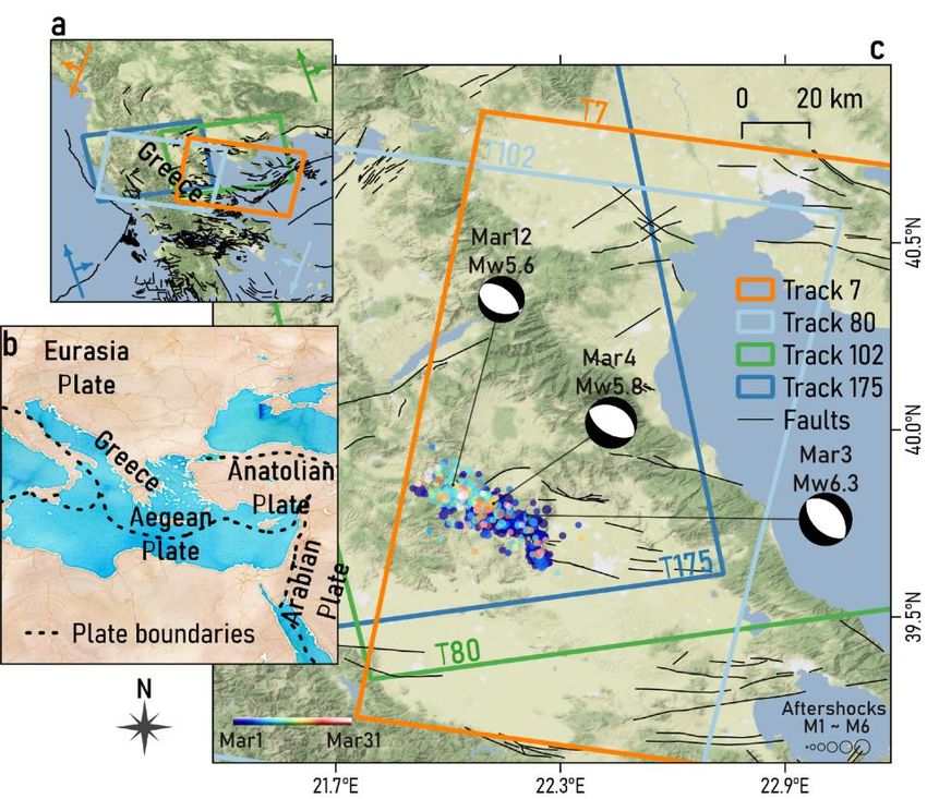
Submitted to Journal of Geodesy

 1   Abstract

 2   Multi-track InSAR data have been widely applied to decompose 2D (East-West and Up-Down)

 3   co-seismic deformation in order to intuitively interpret the co-seismic deformation. Most of the

 4   previous efforts well studied the decomposition of single earthquake deformation using a pair of

 5   ascending and descending InSAR data. However, the deformation decomposition of multiple

 6   earthquake events in a short time period is rarely discussed and hard to implement. That's because

 7   it's hard to make sure that deformation related to each earthquake can be imaged by a pair of

 8   ascending and descending track. In this paper, a Pseudo-Small BASeline (SBAS) method is

 9   developed to decompose 2D deformation of each earthquake in a sequence event. The rationale

10   behind is that several interferograms with different imaging geometries contain co-seismic

11   deformation related to single or multiple earthquakes, and it provides us the opportunity to separate

12   the 2D deformation of a single or multiple events by fusing the short temporal baseline

13   interferograms from multi-track and multi-temporal SAR observations. The proposed method has

14   two parts. The first part is to correct phase unwrapping errors using a compressed sensing method

15   based on redundant SBAS interferograms. In the second part, we incorporate strain model and the

16   conception of SBAS technique into 2D deformation decomposition. We used our proposed

17   Pseudo-SBAS method and four tracks Sentinel-1 data to study the deformation decomposition of

18   an earthquake sequence hit the Central Greece in March 2021. The comprehensive comparisons

19   on synthetic and real Sentinel-1 data confirm the validity of the proposed method. The

20   experimental results also indicate that a triggering mechanism of cascading rupture process can

21   explain the occurrence of these three sequent earthquakes, and the decomposed post-seismic

22   deformation of the first earthquake in EW direction move towards the opposite direction to the co-

23   seismic deformation.

                                                       2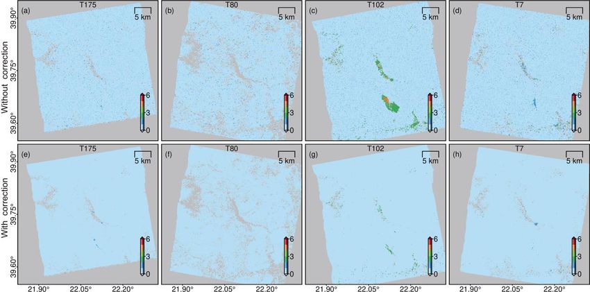
Submitted to Journal of Geodesy

 1   Key words—Co-seismic Deformation, SAR interferometry (InSAR), Compressed Sensing, Strain Model,

 2   Small Baseline (SBAS), Central Greece Earthquake Sequence.

 3   1 Introduction

 4   In UTC time of 2021 March 3 10:16, March 4 18:38 and March 12 12:57, three sequent

 5   earthquakes with Mw6.3, Mw5.8 and Mw5.6 hit the northern Thessaly, Central Greece

 6   (https://earthquake.usgs.gov/earthquakes/eventpage/us7000df40/executive). Previous researches

 7   reported that the well-known and studied faults in Central Greece did not generate these earthquake

 8   sequences (Tolomei et al., 2021). These earthquakes are likely to occur on unmapped or named as

 9   blind faults . Determining the fault geometry of these blind faults is the significant premise for

10   studying earthquake physics and understanding regional seismogenic mechanism (Belabbès et al.,

11   2009; Ghayournajarkar & Fukushima, 2020). Densely spatiotemporal Interferometric Synthetic

12   Aperture Radar (InSAR) measurements lit a lamp for determining fault parameters in those regions

13   only with sparse Global Navigation Satellite System (GNSS) observation, but simultaneously

14   determining the striking and dipping direction for an unmapped or named as blind fault are still

15   challenging, especially for earthquake events only with moderate magnitude (< Mw 7) (Akoglu et

16   al., 2006). Moreover, InSAR technique can only capture 1D surface displacement along the line-

17   of-sight (LOS) direction. When earthquakes did not rupture the surface, it is hard to distinguish

18   fault trace and even the dipping direction from a “visual deceptive” 1D displacement because

19   reported cases revealed that different mechanisms can cause the identical 1D LOS displacements

20   (J. Hu et al., 2014; Sandwell et al., 2000). The issues mentioned above can be potential solved

21   using multi-dimensional deformations (Fialko et al., 2005; Fialko et al., 2001; Jun Hu et al., 2021).

22   Integrating ascending and descending InSAR measurements with different viewing geometries can

23   generate 2D (East-West and Up-Down) deformation to avoid visual fraud in parameters

                                                       3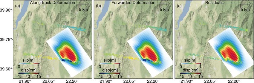
Submitted to Journal of Geodesy

 1   determination (Zheng et al., 2020). However, there still existing some shortcomings in existing

 2   methods in 2D decomposition of sequence earthquake events. A sequence of earthquakes

 3   occurring on adjacent blind faults in a short time period can make determination more complicate.

 4   This is because an interferogram of a 6-day temporal baseline (like Sentinel-1A/B) may include

 5   co-seismic deformation associated with multiple earthquakes and even their early post-seismic

 6   deformation. The ideal case is that both ascending and descending data are perfectly acquired

 7   between each earthquake event. But even for a polar-orbiting satellite constellation like Sentinel-

 8   1, its repeat cycle is at least 6 days (De Zan & Guarnieri, 2006). Exact corresponding ascending

 9   and descending data are hard to achieve. The Central Greece earthquake sequences exactly is

10   facing this challenge. We can see from Table 1 and Fig.S1, in which all possible Sentinel-1 multi-

11   track and multi-temporal interferograms are listed, only the Mw 5.6 event has a pair of ascending

12   and descending interferograms only including the related event’s co-seismic deformation. For

13   another two events, the simultaneously existing ascending and descending data which only

14   corresponds to a single event are absent.

15                                            TABLE I
16        RECORDS OF EARTHQUAKE SEQUENCE AND TIME NODES OF REDUNDANT SBAS INTERFEROGRAMS
                                       Date
                Track                                      Mw6.3      Mw5.8      Mw5.6
                               (yyyymmdd-yyyymmdd)
                                20210302-20210308            ●          ●          ○
               T175                                          ●          ●          ●
                                20210302-20210314
             Ascending                                       ○          ○          ●
                                20210308-20210314
                                20210302-20210308            ●          ●          ○
               T80                                           ●          ●          ●
                                20210302-20210314
            Descending                                       ○          ○          ●
                                20210308-20210314
                                20210225-20210303            ●          ○          ○

                                20210225-20210309            ●          ●          ○

               T102             20210225-20210315            ●          ●          ●

             Ascending          20210303-20210309            ○          ●          ○

                                20210303-20210315            ○          ●          ●

                                20210309-20210315            ○          ○          ●

                                20210225-20210303            ○          ○          ○

                                20210225-20210309            ●          ●          ○
                T7                                           ●          ●          ●
                                20210225-20210315
            Descending                                       ●          ●          ○
                                20210303-20210309
                                20210303-20210315            ●          ●          ●

                                                      4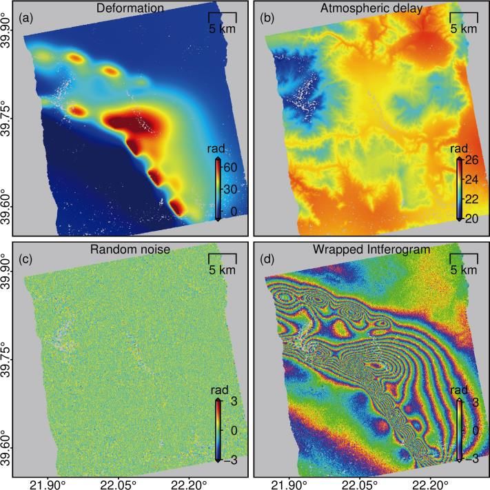
Submitted to Journal of Geodesy
20210309-20210315 ○ ○ ●
1 ● cover ○ not cover
2 To recover 2D surface deformation related to each earthquake, we proposed a Pseudo small
3 BASeline (SBAS) method which inherits the idea of the ordinary SBAS technique (Berardino et
4 al., 2002). Its novelty and behind rationale are to decompose 2D deformation of each event through
5 fusing interferograms generated from multi-track and multi-temporal SAR images. Before
6 accurately decomposing 2D deformation, there are two issues that need to be further solved, which
7 are rarely discussed in decomposing 2D deformation from a single pair of ascending and
8 descending interferograms.
9 The first is unwrapping errors occurring in co-seismic interferograms. Phase discontinuities caused
10 by noise and fast phase variation due to steep co-seismic deformation gradient and atmospheric
11 turbulence can potentially result in phase unwrapping (PU) errors (Chen & Zebker, 2002;
12 Costantini, 1998; Dennis C Ghiglia & Pritt, 1998; Dennis C. Ghiglia & Romero, 1996; Goldstein
13 et al., 1988; F. Liu & Pan, 2020; Xu & Sandwell, 2020; H. Yu et al., 2017; H. Yu et al., 2019;
14 Yunjun et al., 2019; Zebker & Lu, 1998). These errors will lead to a few centimeters of incorrect
15 co-seismic deformation estimated in the interferograms, which will potentially lead to a
16 misestimation of co-seismic slip and seismic moment in the following geophysical inversion
17 process. Triplet phase closure check has proved its validity in PU error detection and correction
18 (Biggs et al., 2007). The rationale behind is that triplet loops of redundant SBAS interferograms
19 can help to check the phase consistency of spatially unwrapped phases. After establishing a linear
20 relationship between the incidence matrix of SBAS interferograms and integer triplet phase closure
21 cycles ( 2 , one cycle), an integer linear programming (ILP) method (Ma et al., 2021) can be
22 implemented pixel by pixel in space to calculate the unwrapping errors. It reformulates the problem
23 of integer unwrapping error correction under the mathematical framework of compressed sensing
5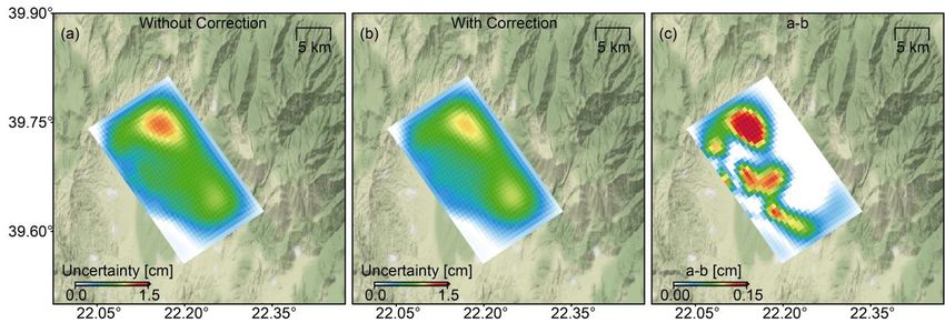
Submitted to Journal of Geodesy

 1   (CS) technique (Donoho, 2006) and replace the nonconvex discontinuous L0-Norm by the convex

 2   continuous L1-Norm, leading to a L1-Norm ILP, further a good correction performance (Candes &

 3   Tao, 2005).

 4   The second issue to be solved is that an interpolation operation of interferograms for each track

 5   data is needed. The deformation decomposition is in a pixel-wise way, while the pixels of each

 6   track data are not in unique positions (Jihong Liu et al., 2019). An interpolation process such as

 7   bilinear or cubic is required. For those pixels with unwrapping errors and atmospheric turbulence,

 8   interpolation however will distort measurements (J. Liu et al., 2018). Strain model method which

 9   can simultaneously retrieve 2D/3D deformation and strain tensor is proposed to avoid the

10   interpolation process (Jun Hu et al., 2021). It further considers the spatial correlation of

11   neighboring pixels according to the elastic deformation theory (Guglielmino et al., 2011). Even in

12   a small region without points, the deformation of this region can still be inferred by the adjacent

13   points. Therefore, resampling process can be avoided when incorporating strain model in the

14   decomposition. In summary, our proposed Pseudo-SBAS method to decompose 2D deformation

15   incorporates SBAS technique, ILP correction and strain model. In this context, decomposed 2D

16   surface deformation for each earthquake using Pseudo-SBAS method is helpful to constrain the

17   fault parameters for each earthquake and further interpret seismogenic mechanisms.

18   This article is organized as follows. Section 2 describes the tectonic setting, the used data and

19   motivation in details. Section 3 introduces the proposed Pseudo-SBAS method. We test the

20   performance of the developed algorithm using synthetic and real Sentinel-1 data in Section 4 and

21   5, respectively. Discussions on the experimental results and Pseudo-SBAS are given in Section 6.

22   Finally, Conclusions are outlined in Section 7.

                                                       6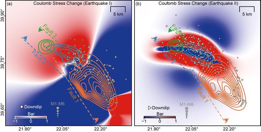
Submitted to Journal of Geodesy

 1   2 Tectonic Settings, data preparation and motivation

 2   These sequent earthquakes occurred in a region where no-ever mapped faults with significant

 3   deformation has been recognized (Fig.1c). The central Greece is one of the most active tectonic

 4   regions of Aegean region resulted from landmass collision between outer Hellenides and the

 5   Adriatic microplate (Fig.1b) (Papazachos & Delibasis, 1969). This fault zone consists of many

 6   parallel synthetic and antithetic fault segments with a mean ENE-WSW trending direction of

 7   shortening and a dominantly NE-SW extensional stress. In consequence, central Greece is

 8   dominated by conjugate system of normal faults with general directions NW-SE and NE-SW (R.

 9   Caputo et al., 2004; Riccardo Caputo & Pavlides, 1993). Moreover, seismological data indicate

10   that strong earthquakes are mostly associated with the conjugate system (Papadimitriou &

11   Karakostas, 2003). From the large tectonic background (Fig.1b), the northward movement of the

12   African plate and the compression of the Eurasian plate resulted in active tectonics in Aegean Sea

13   zone. Therefore, the northward motion of the Arabian plate pushes the smaller Anatolian plate

14   westwards along the North Anatolian fault (NAF), continuing along the North Aegean trough

15   (NAT) region, which is the boundary between the Eurasian and south Aegean plates (McKenzie,

16   1978; Papadimitriou & Sykes, 2001), absorbing most compression of the northward motion.

17   Normal faults with right-lateral shear motion associated with the NAF appears to become more

18   distributed in north Greece boundary, but transferred into N-S or NW-SE direction. Furthermore,

19   the Holocene alluvial deposits in Upper Pleistocene accelerated the formation of distributed NW-

20   SE trend basin in central Greece (Demitrack, 1986), which managed most of the earthquake events

21   in this region. The occurrence of these three earthquakes may be triggered by the movement of

22   NW-SE of regional tectonics.

23

                                                      7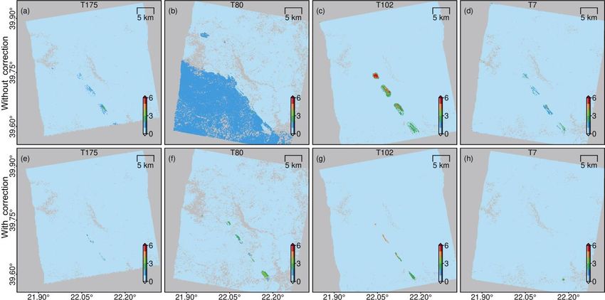
Submitted to Journal of Geodesy

 1

 2   Fig.1. Tectonic settings and Sentinel-1 tracks coverage of the study area. (a) describing the coverage of four tracks data; (b) showing the plate

 3   boundaries around Greece. (c) is the zoomed-in-view of the study region covering three sequent earthquakes.

 4

 5   Four tracks of Sentinel-1 TOPS data covering Thessaly, Central Greece region are used for

 6   inverting 2D deformation of the earthquake sequence. In ascending track 175, we formed 3

 7   interferograms from three SAR acquisitions: 20210302, 20210308 and 20210314. In descending

 8   track 80, we generated 3 interferograms from three SAR acquisitions: 20210302, 20210308 and

 9   20210314. In ascending track 102, 6 interferograms are obtained from four SAR acquisitions:

10   20210225, 20210303, 20210309 and 20210315. In descending track 7, 5 interferograms are

11   generated from four SAR acquisitions: 20210225, 20210303, 20210309 and 20210315.

12   Pioneering researches on the 2021 central Greece March earthquake sequence inverted 2D

13   deformation of total three earthquakes using two interferograms generated from tracks 80 and 175

14   (02 Mar 2021 - 14 Mar 2021)(Tolomei et al., 2021). The inverted 2D deformation maps contain

                                                                            8
Submitted to Journal of Geodesy
1 the cumulative co-seismic deformation of three earthquakes and early post-seismic deformation.
2 Subsidence dominates the maximum displacement in UD, and a small cumulative uplift locates
3 around the subsidence. Similar to it, the asperities of inverted cumulative EW deformation also
4 overlap with each other. It is hard to determine the deformation caused by each earthquake. Thus,
5 in order to isolate the deformation of three respective earthquakes, previous efforts only use
6 interferograms containing a single co-seismic deformation to study the slip distribution of each
7 earthquake. Those interferograms containing multiple seismic deformations were discarded. In
8 previous studies (Ganas, Valkaniotis, Briole, et al., 2021; Papadopoulos et al., 2021), it has been
9 pointed out that there may be a domino-like triggering mechanism between the three earthquakes.
10 In addition, the Mw 6.3 earthquake was accompanied by significant post-seismic deformation, and
11 these deformations are likely to disturb the geodetic inversion of subsequent earthquakes. In this
12 context, deformation maps of each earthquake which isolate the effects of other events is of great
13 significance for further revealing the triggering mechanism and accurate slip inversion. To this
14 end, we proposed Pseudo-SBAS method to accurately invert 2D deformation associated with each
15 earthquake. Based on it, the fault geometry, underlying mechanism and the characteristics of post-
16 seismic deformation are further revealed.
17 3 Methodology
18 3.1 Integer Linear Programming for Phase Unwrapping Error Correction
19 Triplet phase closure check has proven its capability in phase unwrapping error detection (Biggs
20 et al., 2007; Fattahi, 2015). For a triangle loop of three unwrapped interferograms 1,2 , 1,3 and
21 2,3 obtained from three SAR acquisitions 1, 2 and 3, the corresponding phase closure 1,2,3 is
22 defined as
9Submitted to Journal of Geodesy
1,2,3 = 1,2 + 1,3 2,3 (1)
.
1 When the interferograms are contaminated by phase unwrapping errors, 1,2,3 will not be equal to
2 0. We can list the triplet phase closure of all triangles in the SBAS graph as . Then we can
3 construct a linear equation to build the relationship between unwrapping errors to be corrected and
4 closure phases. Its mathematical formulation can be described as
BN M X M 1 =round ( ) N 1
2 . (2)
X M 1 ¢
5 where B is the incidence matrix generated by SBAS graph, round ( ) means the integer cycles of
2
6 unwrapping errors, X represents the ambiguity cycles for each interferogram to be corrected, N is
7 the number of triangle loops and M is the number of interferograms. In ordinary SBAS graphs, N
8 is usually less than M. To illustrate, three interferograms can only construct one triangle loop.
9 Therefore, the solution search for (2) is a rank-deficient problem. To search for an optimal solution
10 to (2) and ensure the solution are all integers, L-0 norm is the best objective function when we
11 assume that part of interferograms contain no unwrapping errors. In this context, the solution
12 search for (2) turns out to be a sparse signal recovery problem. L-0 is hard to approach because it
13 is not a non-convex optimization problem. In our previous effort (Ma et al., 2021), we convert (1)
14 into a L-1 norm to approach the superiority of L-0 norm:
X
BN M BN M M 1 =round ( ) N 1
X M 1 2
X M 1
s.t. min (3)
X M 1 1 .
X M 1 X M 1 X M 1
X M 1 , X M 1 ¥ 0
10Submitted to Journal of Geodesy
1 where X M 1 and X M 1 are natural numbers including zero. It can be seen from (3) that this
2 reformulation of (2) limits the solution search range to natural numbers including zero instead of
3 all integers. Therefore, the complexity of solution search has a sharp drop (Candes & Tao, 2006).
4 Equation (3) can be solved by the integer linear programming (ILP) method which incorporates
5 Branch and Cut, Presolve and parallel computing techniques. In this study, we use the subroutine
6 “intlinprog.m” of MATLAB (https://ww2.mathworks.cn/help/optim/ug/intlinprog.html) as a
7 toolbox to solve this L-1 norm optimization problem.
8 3.2 2D Deformation Decomposition Using Pseudo-SBAS
9 Through the comparison of recorded earthquake time from Fig.S1 and Table 1, one can see that
10 only T102 recorded independent co-seismic deformation of three earthquakes. Except for one
11 interferogram in T7 that does not record any surface deformation (we excluded it in the following
12 experiments), all other interferograms contain the surface deformation related to at least one
13 earthquake. For each earthquake event, one ascending interferogram and one descending
14 interferogram only including the associated deformation are unachievable. To recover surface
15 deformation related to each earthquake, we borrow the idea of SBAS technique. For a better
16 illustration, we give a mathematical description about its realization. This process can be formed
17 by a linear equation of L B A X :
11Submitted to Journal of Geodesy
LT1 175 aT 175 bT 175 aT 175 bT 175 aT 175 bT 175
T 175 T 175
L2 a bT 175 aT 175 bT 175 aT 175 bT 175
LT3175 aT 175 T 175
X e1
T 80 T 80
bT 175 aT 175 bT 175 aT 175 b 1
Xu
L1 a bT 80 aT 80 bT 80 aT 80 bT 80 X e2
M
M M M M M M A176 2
Xu
LT6102 aT 102 bT 102 aT 102 bT 102 aT 102 bT 102 X3
T7 T7 . (4)
L2 a bT 7 aT 7 bT 7 aT 7 bT 7 e
M M X u3
M M M M M
T7 T7 X 61
L6 a bT 7 aT 7 bT 7 aT 7 bT 7
L171 B176
3
a sin( ) cos i , bi cos i , i T 175, T 80,T 102,T 7
i i
2
1 where Lij is the jth interferogram in i track, i and i are respectively the azimuth and incidence
2 angle for i track, X ei and X ui each means the surface deformation associated with ith earthquake
3 event in EW and UD direction, is the Hadamard product, A is the incidence matrix which
4 converts surface deformation into LOS displacement L in combination with projection matrix B.
5 A is defined as
1 1 0 1 1 0 1 1 1 0 0 0 1 1 1 1 0
1 1 0 1 1 0 1 1 1 0 0 0 1 1 1 1 0
0 0 0 1 1 0 0
A 1
T 1 1 1 1 1 1 1 1 1
(5)
1 1 0 1 1 0 0 1 1 1 1 0 1 1 1 1 0
0 1 1 0 1 1 0 0 1 0 1 1 0 1 0 1 1
0 1 1 0 1 1 0 0 1 0 1 1 0 1 0 1 1
6 where T means matrix transpose operation.
7 Before getting (4) to work, there is still a left issue. That is the solution process of (4) is pixel-wise
8 but the selected pixels of each track are not in unique positions. Strain model can be introduced to
9 solve this issue. In its realization, a transformation matrix representing correlation between
10 neighboring pixels is used to convert L B A X which only supports for one pixel to neighboring
11 pixel gathers. That is
12Submitted to Journal of Geodesy
L Ggeo L B176 m A176 m Ggeo,6 m8 X 81
1 0 xe
i
xni xui 0 0 xui
0 1 0 0 xei xni xui xei
0 xe
i
xni xui 0 0 xui
Gi
1 (6)
xei xni xui xei
geo
0 1 0 0
xui
0 xe xni xui
i
1 0 0
0 1 0 0 xei xni xui xei 68
xei xei xec , xni xni xnc , xui xui xuc
1 where represents the neighboring m points in a defined distance threshold, Ggeo is the
2 transformation matrix based on strain model, i means the ith pixel in , and xni , xei and xui
3 respectively represent the distance of ith pixel between the center pixel c in north, east and vertical
4 directions. In this study, we set the distance range to 200 m. Unlike other techniques adopting
5 strain model, we did not adopt variance component estimation to determining weight matrix for
6 all measurements because the measurements we used are all from a unique platform rather than
7 from different satellites with totally different viewing geometries. Instead, we used an iterative
8 reweighting least squares (IRLS) method to complete it.
9 3.3 Summary of the Pseudo-SBAS Workflow
10 The proposed Pseudo-SBAS workflow pursues a 2D deformation decomposition scheme through
11 fusing multi-track SAR observations. In summary, this whole workflow shown in Fig.2 consists
12 of three detailed steps: 1) phase unwrapping error correction, 2) construct strain model, and 3)
13 pixel-wise solution search. In the first step, triplet phase closure (Eq. (1)) check is used to detect
14 phase unwrapping errors occurring in redundant interferograms. Then ILP (Eq. (3)) is applied to
15 solve the unwrapping errors and add back to all interferograms. In the second step, all ascending
16 and descending tracks data are used to construct the strain model using Eq. (6). The radius for
17 neighboring point search is set to 200 m. In the third step, IRLS is used to solve Eq. (6) for all
18 points.
13Submitted to Journal of Geodesy
1
2 Fig.2. Schematic diagram of the proposed Pseudo-SBAS workflow.
3 4 Synthetic data experiment
4 4.1 Simulation process
5 Synthetic data provides us a great opportunity for testing the validity of our proposed Pseudo-
6 SBAS method, as all true values are known. We simulated four track InSAR data consisting of 17
7 interferograms as shown in Table 1. The simulated T175, T80, T102 and T7 track data respectively
8 consists of 2920220, 1522164, 3292112 and 3218798 sparse points, distributed same as the real
9 data selected by an empirical coherence threshold of 0.75. The simulated incidence and azimuth
10 angles of these four tracks data are all inherited from and consistent with the real data, aiming to
11 simulate the LOS geometry as close as possible to the real data. The synthetic deformation phase
12 is simulated by three checkboard simulations based on three inferred fault models and Okada85
14Submitted to Journal of Geodesy
1 green functions (Okada, 1985), as shown in Fig. S2. We set the rake angles of three slip models to
2 -90 degrees to simulate the normal dipping slip. The simulated seismic moments of three slip
3 models are corresponding to Mw 6.3, Mw 5.8 and Mw 5.6, respectively. The simulated
4 atmospheric phases of 17 interferograms are based on the tropospheric delay maps provided by
5 GACOS system (Generic Atmospheric Correction Online Service for InSAR) (C. Yu et al., 2018).
6 We also added random errors with a standard deviation of 1cm 3-sigma to 17 simulated
7 interferograms. 17 simulated interferograms are shown in Fig.S3.
8 Furthermore, we give an example interferogram in Fig.3 to better illustrate the simulation process.
9 Fig.3(a) shows the simulated deformation in radians generated by Okada85 model. Fig.3(b) shows
10 the simulated atmospheric delay generated from GACOS system. Fig.3(c) presents the random
11 noise. Fig.3(d) shows the wrapped interferogram containing all phase components of (a-c).
12
13 Fig.3. The simulated phase components of an exemplary interferogram (T102 20210225-2021015). (a) simulated deformation phase in radian; (b)
14 simulated atmospheric phase delay in radian; (c) simulated random noise in radian; and (d) wrapped interferogram consisting of (a-c).
15Submitted to Journal of Geodesy
1 4.2 Simulation process
2 In order to validate the performance of phase ambiguity correction using ILP, we first unwrap 17
3 simulated interferograms using APSP-MCF method (All-Pair-Shortest-Path Minimum Cost
4 Flow). In APSP-MCF, Delaunay and KNN (K-Nearest Network) are first generated. Based on the
5 edge set of Delaunay and KNN network, temporal coherence of all edges are computed and then
6 APSP algorithm is used to search for a network with the maximum temporal coherence (M. Jiang
7 & Guarnieri, 2020). Because the temporal coherence is calculated by the phase gradient of all
8 edges in the time domain, the higher the temporal coherence is, the smaller the phase gradient is.
9 Therefore, phase continuity assumption can be easier to satisfy and a good PU performance can
10 be achieved. More details about the outperformance of APSP-MCF to other state-of-the-art
11 techniques can be obtained from (Ma et al., 2021).
12 After APSP-MCF, 17 unwrapped interferograms are shown in Fig.S4. We checked all triplet phase
13 closures for four tracks and presented the related sum of absolute closure cycles in Fig.4a. Based
14 on the calculated triplet phase closure, we constructed the linear equation between SBAS graph
15 and PU error ambiguity cycles to be corrected. Then ILP is used to search for the final solution.
16 All searched ambiguity cycles are added back to the unwrapped interferograms. We calculated the
17 triplet phase closure of the corrected interferograms (Fig.S5) and presented them in Fig.4b. Given
18 that the less phase closure cycles, the higher PU accuracy is, the corrected interferograms show a
19 good performance. The closure cycle number of four tracks show obvious closure cycles near fault
20 trace before correction. These unwrapping errors are likely resulted by the steep phase gradient
21 introduced by our simulated near-surface slip asperities. These near-surface slips mimic what
22 would happen if an earthquake ruptured the surface. Instead, the closure cycle number of four
23 tracks data are all close to zero after correction. This is because these areas with unwrapping errors
16Submitted to Journal of Geodesy
1 exist only in part of SBAS interferograms. We can see it from Figs.S6 and S7. The locations with
2 unwrapping errors did not show up on all interferograms. The sparsity premise of compressed
3 sensing is satisfied, therefore ILP can work well (Ma et al., 2021).
4
5 Fig.4. The sum of absolute triplet phase closure cycles. (a-d) represents the results of T175, T80, T102 and T7 without phase unwrapping error
6 correction respectively. (e-h) are the results of four tracks interferograms after correction in the same order.
7 4.3 Performance of Pseudo-SBAS in 2D Deformation Decomposition
8 After phase unwrapping error correction, 2D deformation decomposition can be performed based
9 on these high-quality observations. To validate the accuracy of Pseudo-SBAS, we compare its
10 decomposed deformation maps with three other methods: the bilinear interpolation method based
11 on these interferograms without unwrapping error correction, strain model method based on
12 interferograms without error correction, the bilinear interpolation method based on interferograms
13 with error correction. The bilinear interpolation-based method directly interpolates all
14 interferograms to a unique reference and then decompose 2D deformation using least squares
15 method.
17Submitted to Journal of Geodesy
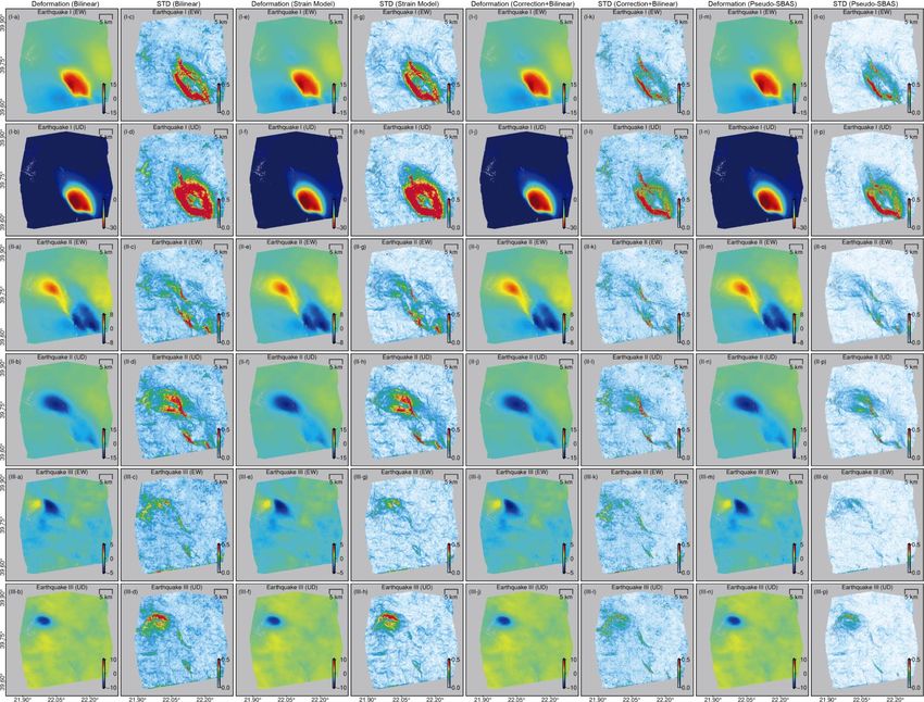
1 We compare the results of these four methods in Fig.5. The decomposed 2D deformation by
2 bilinear+uncorrection method are shown in Fig.5(Ia-b, IIa-b, IIIa-b) and their corresponding errors
3 between true values are shown in Fig.5(Ic-d, IIc-d, IIIc-d). 2D deformation maps decomposed by
4 strain model+uncorrection are shown in Fig.5(Ie-f, IIe-f, IIIe-f) and their related errors are shown
5 in Fig.5(Ig-h, IIg-h, IIIg-h). 2D deformation decomposed by bilinear+correction method are
6 presented in Fig.5(Ii-j, IIi-j, IIIi-j) and their corresponding errors between true values are shown
7 in Fig.5(Ik-l, IIk-l, IIIk-l). Deformation maps decomposed by strain model+correction (Pseudo
8 SBAS) are shown in Fig.5 (Im-n, IIm-n, IIIm-n) and their corresponding errors are shown in
9 Fig.5(Io-p, IIo-p, IIIo-p). It can be seen from the error maps that the larger deformation errors
10 decomposed by bilinear method occur in areas where the unwrapping errors exist. These estimated
11 deformation errors are reduced by ILP correction method. In addition, the errors in other areas are
12 also significantly reduced. It directly due to strain model in Pseudo-SBAS. It considers the elastic
13 theory to incorporate neighboring observations into pixel-wise deformation decomposition.
14 Therefore, it is more resistant to the effects of error. Generally, Pseudo SBAS method can achieve
15 the most accurate deformation maps compared with other three methods. To further validate the
16 performance of strain model in Pseudo SBAS and give a statistical result on it, we perform a Monte
17 Carlo test described in the below subsection.
18Submitted to Journal of Geodesy
Fig.5. The decomposed 2D deformations maps related to three earthquakes. I, II and III represent three earthquakes. (a-b), (e-f), (i-j) and (m-n) are respectively the EW and UD deformation. (c-d), (g-h), (k-l) and (o-p) are are their difference
from true values. The 1-2, 3-4, 5-6 and 7-8 column respectively represent the results of the bilinear, strain model, correction+bilinear and Pseudo SBAS mthod.
19Submitted to Journal of Geodesy
1 4.4 Error Resistance Capability of Strain Model in 2D Deformation Decomposition
2
3
4 Fig.6. Statistical results of two methods in 2D deformation decomposition.
5 To validate the error resistance capability of strain model in Pseudo-SBAS, a Monte-Carlo
6 simulation test is carried out. We added random noise with different magnitudes to 17 simulated
7 interferograms. In order to eliminate the effect of the unwrapping errors, we did not unwrap the
8 simulated interferograms, but directly decompose the 2D deformation with the simulated
9 interferograms. The random noise STD is set to a range from 0 to 1.5 3-sigma. In addition, we also
10 add atmospheric delay phase with different magnitudes in interferograms. It means that the strain
11 model has to deal with two different kinds of errors, one is random and the other is with long
12 wavelength characteristics. In the first case, we only add the atmospheric phase equal to the phase
13 delay provided by GACOS. In the second case, we magnify the phase delay to double.
20Submitted to Journal of Geodesy
1 We compare bilinear interpolation method as a benchmark. It can be seen from Fig.6 that the
2 bilinear interpolation method is obviously less resistant to two kinds of noise than the strain model
3 in both EW and UD direction. With respect to the accuracy of deformation decomposition in two
4 directions for two methods, UD is obviously higher than that EW. This is because vertical
5 deformation components contribute more to LOS direction. This also makes the vertical direction
6 more sensitive to changes in atmospheric error magnitude, as can be seen from the increase in (root
7 mean square error (RMSE). With the increase of atmospheric delay, the RMSE of UD direction
8 increased by about 0.25cm, while the EW direction increased by less than 0.1cm. However, the
9 RMSE increase of strain model is much lower than that of bilinear interpolation method when the
10 magnitude of random noise and atmospheric phase delay increases. It validates the error resistance
11 capability of our proposed method.
12 5 Real data experiment
13 5.1 Interferometric Processing
14 By following the standard TOPS interferometric processing, we processed all interferograms using
15 our proposed Minimum-Spanning-Tree Enhanced Spectral Diversity (MST-ESD) method (Ma et
16 al., 2019). In MST-ESD, we first performed a geometrical co-registration method (Sansosti et al.,
17 2006) using external Digital Elevation Model (DEM) and precise orbit to resample all images to a
18 common reference, then we used MST method to select high signal-to-noise ratio (SNR)
19 interferogram pairs. For those robust pairs, we perform ESD technique to correct the residual
20 azimuth mis-registration. Noted that when image number in a same track is less than 4, MST-ESD
21 is degenerated to single-reference method. After co-registration tasks, we simulated the flat-earth
22 phase using orbit and DEM and removed them from processed 14 SLCs. In this step, we also
21Submitted to Journal of Geodesy
1 generated latitude, longitude and incidence pixel-wisely. Then we generated all possible
2 interferograms, 17 in all. We multi-looked all interferograms with a factor of 1 by 4 respectively
3 in the azimuth and range direction, resulting a grid resolution of ~13 m by ~13m. 17 interferograms
4 were then filtered by an adaptive Goldstein filter (Mi Jiang et al., 2014) and we masked out low
5 coherence areas with a mean coherence less than an empirical value of 0.75. After pixel selection,
6 we unwrapped all interferograms using APSP-MCF. Then phase unwrapping errors are
7 automatically detected based on triplet phase closure and ILP is used to mitigate those detected
8 unwrapping errors.
9 5.2 Performance of ILP PU Error Correction
10 In order to validate the performance of phase ambiguity correction using ILP in real data
11 experiment, we chose the same quality indicator as Section 4.2: the sum of absolute closure cycles
12 before and after correction. We present the results in the below Fig.7. Fig.7a-d demonstrate the
13 associated results before correction, and Fig.7e-h present the related results after correction. As
14 expected from Section IV-B, the sum of closure cycle number of corrected interferograms show
15 obviously less closure cycles than interferograms without correction, especially in the near filed
16 of T102. A large area where ambiguity cycles reach at least 3 gets close to zero after correction. It
17 validates the effectiveness of ILP in real data.
18
22Submitted to Journal of Geodesy
1
2 Fig.7. The number of absolute triplet phase closure cycles. (a-d) represents the results of T175, T80, T102 and T7 without phase unwrapping
3 error correction respectively. (e-h) are the results of four tracks interferograms after correction in the same order.
4 5.3 Performance of Pseudo-SBAS in 2D Deformation Decomposition
5 Based on 17 corrected interferograms, we decompose 2D deformation related to three sequent
6 earthquakes using four methods in Section 4.3. In order to validate the accuracy of these
7 decomposed deformation maps, we chose the standard deviation (STD) of 2D deformation maps
8 in a radius of 200m as a quality indicator. Assuming the co-seismic deformation varies little in a
9 short distance, the deformation STD will get close to zero if little noise exists. We present the
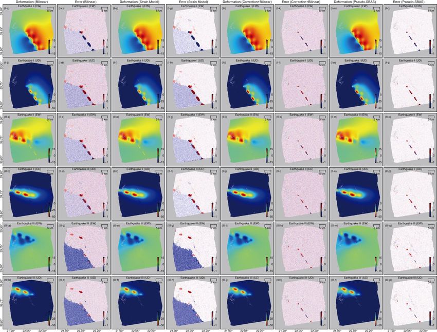
10 deformation maps and their related STD results in the below Fig.8. The decomposed 2D
11 deformation by bilinear+uncorrection method are shown in Fig.8(Ia-b, IIa-b, IIIa-b) and their
12 corresponding STD are shown in Fig.8(Ic-d, IIc-d, IIIc-d). 2D deformation maps decomposed by
13 strain model+uncorrection are shown in Fig.8(Ie-f, IIe-f, IIIe-f) and their related STD are shown
14 in Fig.8(Ig-h, IIg-h, IIIg-h). 2D deformation decomposed by bilinear+correction method are
15 presented in Fig.8(Ii-j, IIi-j, IIIi-j) and their corresponding STD are shown in Fig.8(Ik-l, IIk-l, IIIk-
16 l). Deformation maps decomposed by Pseudo SBAS are shown in Fig.8(Im-n, IIm-n, IIIm-n) and
23Submitted to Journal of Geodesy
1 their STD are shown in Fig.8(Io-p, IIo-p, IIIo-p). As expected, the STD of deformation maps
2 derived by Pseudo-SBAS show obviously less values than that derived by bilinear method. In the
3 near field region, the deformation STD is relatively large, which is reasonable because the near
4 field deformation gradient is large and the deformation changes in short space distances can be
5 steep. But for the far field where are mainly affected by noise, the STD contrast is very obvious.
6 The mean STD value reduction of the results of Pseudo-SBAS can validates it capability in error
7 resistance. To further validate its superiority in deformation decomposition, we present four RMSE
8 maps in Fig.9 to demonstrate the outperformance of Pseudo-SBAS. These four maps are obtained
9 from the model residuals when solving (6). The less RMSE, the decomposed deformation maps
10 are more consistent with the inversion model in (6), which also indicates that the inversion model
11 is more reasonable.
24Submitted to Journal of Geodesy
Fig.8. The decomposed 2D deformations maps related to three earthquakes. I, II and III represent three earthquakes. (a-b), (e-f), (i-j) and (m-n) are respectively the EW and UD deformation. (c-d), (g-h), (k-l) and (o-p) are are their STD.
The 1-2, 3-4, 5-6 and 7-8 column respectively represent the results of the bilinear, strain model, correction+bilinear and Pseudo SBAS method.
25Submitted to Journal of Geodesy
1
2 Fig.9 The RMSE values of bilinear and P-SBAS method in the decomposition process. (a) bilinear. (b) Pseudo-SBAS.
3 Through visual inspection on Fig.9, RMSE maps of bilinear method based on uncorrected (Fig.9a)
4 and corrected interferograms (Fig.9c) are both significantly higher than strain model based
5 methods (Fig.9b and Fig.9d). Overall, Pseudo SBAS combines the advantages of unwrapping error
6 correction and strain model to achieve the best performance. Quantitatively, we also calculated the
7 mean RMSE values for four RMSE maps. The mean RMSE of bilinear method is 0.71cm whereas
8 the mean RMSE of bilinear+correction is 0.58cm. The mean RMSE of strain model is 0.63cm.
9 The results derived from Pseudo-SBAS outperforms that derived from other three methods, with
10 a value of 0.52cm. It can validate the higher accuracy of Pseudo-SBAS method.
11 5.4 Validation of Decomposed 2D Deformation of Pseudo SBAS Using Forward Modeling
12 and Burst Overlap Interferometry
13 Although we lack external validation data such as GPS, along-track deformation is used as
14 validation data in this paper. The rationale behind is that we treat the decomposed 2D deformation
26Submitted to Journal of Geodesy
1 maps as the constraint of geodetic inversion, and we forward model the 3D deformation using the
2 inverted slip models. The forwarded 3D deformation can be converted into along-track direction.
3 Then we can compare it to the along-track deformation calculated by burst overlap interferometry
4 (BOI) (He et al., 2019; H. Jiang et al., 2017). BOI, a method developed specifically for Sentinel-1
5 Terrain Observation by Progressive Scan (TOPS) SAR data, has been proven to be sensitive the
6 along-track deformation. In the geodetic inversion, we only used 2D deformation decomposed
7 from LOS observations as constraints. Along-track deformation obtained from BOI is independent
8 of the LOS direction, therefore it can be treated as an objective validation data. In Text S1 and S2,
9 we give detailed descriptions about the geodetic inversion process and the along-track deformation
10 extraction process. Since no significant along-track deformation can be found in moderate
11 earthquakes (Mw < 6) and only T102 includes along-track deformation related to a single event,
12 and thus, we only give a comparison of the results for the first earthquake.
13 We presented the derived slip model and along-track deformation results in Fig.10. In Fig.10a, we
14 overlay the extracted along-track deformation map on the inverted slip model, and in Fig.10b we
15 show the forwarded along-track deformation over the slip model. It can be seen from Fig.10c that
16 their difference is little. We can therefore conclude that the 2D deformation decomposed using
17 Pseudo-SBAS is correct. The proposed Pseudo-SBAS is an effective method in 2D deformation
18 decomposition.
19
27Submitted to Journal of Geodesy
1
2 Fig.10. The derived slip model and along track deformation maps. (a) is the calculated along-track deformation; (b) is the forwarded along-track
3 deformation based on the slip model of the first earthquake; and (c) is their difference.
4 6 Discussions
5 6.1 Effects of Unwrapping Errors on Slip Distribution
6
7 Fig.11. The derived slip model uncertainty using JK tests. (a) is the uncertainty from results without phase unwrapping correction.; (b) is the
8 uncertainty from results with correction; and (c) is their difference.
9 In order to explore the effects of the unwrapping errors on the inversion results, we adopted a JK
10 (Jack-Knife) statistical method to calculate the slip uncertainty of two models constrained by 2D
11 deformation maps without and with unwrapping errors correction (Khoshmanesh et al., 2015). The
12 imperfection of Green's function is caused by simplified fault model and other factors. These
13 regions in the fault model are very sensitive to potential errors in the observations. To further
28Submitted to Journal of Geodesy
1 investigate which region of the derived fault model is sensitive to the unwrapping errors, JK tests
2 are performed. Larger slip uncertainty indicates larger observation errors. In order to only evaluate
3 the effect of the unwrapping errors on it, we did not include the strain model in 2D deformation
4 inversion. We adaptively downsampled the 2D deformation maps without and with correction into
5 irregular triangles (Lohman & Barnhart, 2010). The difference of 2D downsampled deformation
6 maps are presented in Fig.S11. We repeat the geodetic inversion process 100 times, adding a white
7 noise with an average of zero and a standard deviation of 5 cm to downsampled deformation maps
8 in each iteration. We calculate the standard deviation of the results 100 times and take it as the
9 uncertainty of the model (Fig.11). We calculated the difference (Fig.11c) between the uncertainty
10 of uncorrected results (Fig.11a) and corrected results (Fig.11b). It can be seen from Fig.11c that
11 there is an overall uncertainty reduction for results with correction. The largest uncertainty
12 reduction is about 0.15cm. It is confirmed that unwrapping errors can disturb the inverted slip
13 model and unwrapping error correction is helpful to mitigate its disturbance.
14 6.2 Is March 4 Earthquake North Dipping or South Dipping?
15 In a recent report on Central Greece earthquake sequence (Ganas, Valkaniotis, Karasante, et al.,
16 2021; Papadopoulos et al., 2021), a question has been raised about the dipping direction of Mar 4
17 earthquake. It is assumed that the seismogenic fault of this earthquake has two kinds of potential
18 faults: north dipping and south dipping. This question arises from the fact that both faults can
19 interpret the deformation pattern in interferogram (T102, 20210303-20210309) which only include
20 the deformation associated with the second earthquake. Based on the interpretation of the 2D
21 deformation we obtained, we favor the north dipping hypothesis. Descriptions below are our
22 explanation of the argument.
29Submitted to Journal of Geodesy
1 The analysis of 2D deformation maps in Fig.8IIm and Fig.8IIn shows that the Mar 4 earthquake
2 caused significant eastward displacements and subsidence with a maximum value of ~10 cm, and
3 slight subsidence is shown in the southwest and northeast of the uplift region. Part of the westward
4 displacements were also displayed in the northeast of the deformation fields, with a maximum of
5 ~4cm. The EW displacement maps are dominated by the eastward deformation which can be
6 interpreted as the right-lateral movement of the north dipping blind fault or the left-lateral
7 movement of the south dipping blind fault. The vertical displacements are dominated by
8 subsidence, so it supported that the seismogenic fault is normal fault. Therefore, the dipping
9 direction the blind fault cannot be determined only from the visual inspection on 2D deformation
10 maps. A geodetic inversion analysis is further needed.
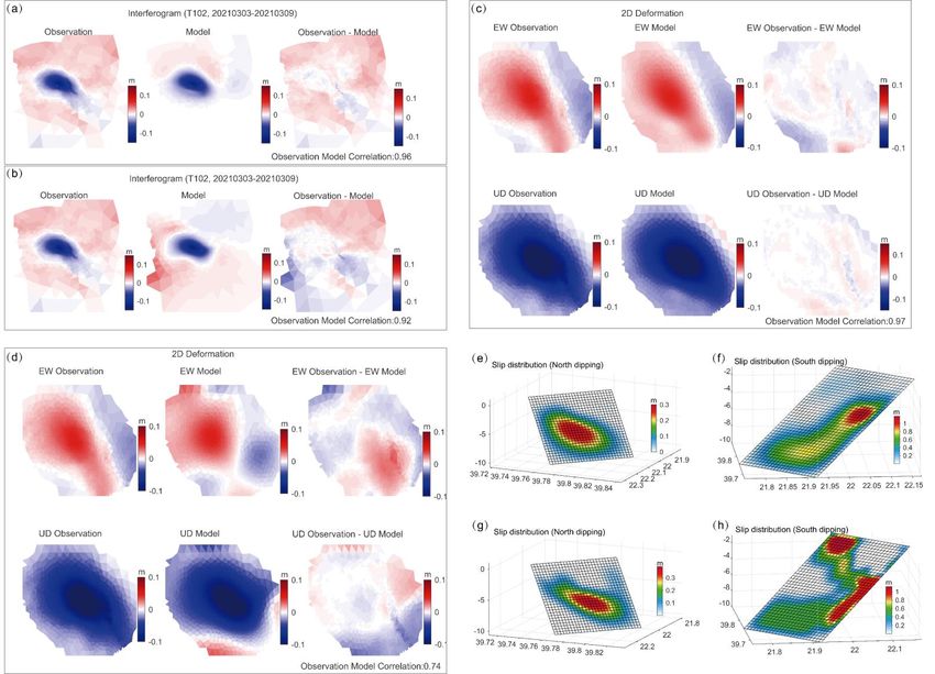
11 In geodetic inversion, 1D interferogram and 2D deformation maps are used as constraints,
12 respectively. It is worth noting that in order to avoid the influence of the post-seismic deformations
13 of Mar 3 earthquake, we extracted out the major co-seismic deformation field of the Mar 4
14 earthquake using an ellipse. Two kinds of rectangular dislocation models of north dipping and
15 south dipping are constructed based on elastic half space. The faults are divided into 700 m by 700
16 m rectangles along the striking and down dipping direction. Fig.12a and Fig.12b present the
17 inversion results of 1D interferogram. It can be seen from the correlation between observation and
18 modeled deformation that the inversion results of two potential faults are good. The lowest data-
19 model correlation also reached 0.92. Their related slip models are presented in Fig.12e and Fig.12f.
20 We also inverted two slip models based on 2D deformations. Their two models based on two
21 different dipping directions are shown in Fig.12g and Fig.12h, respectively. The model (Fig.12g),
22 based on the north dipping fault geometry still maintains a relatively similar shape to the model
23 constrained by 1D interferogram (Fig.12e), which is shaped like an eye. The observations are
30Submitted to Journal of Geodesy
1 consistent with the modeled deformations, and the residuals are small. The data-model correlation
2 reaches 0.97. However, inversion results based on south dipping fault show a low data-model
3 correlation of 0.74. The observations in EW and UD directions are not well consistent with the
4 model, and the residuals are relatively large. The inverted slip model in Fig.12h is inconsistent
5 with the model based on the interferogram. This discrepancy indicates that the geodetic inversion
6 results more support the north dipping hypothesis. It also reflects that the 1D interferogram is not
7 only visually deceptive, but can even cause completely different inversion results. Therefore, 2D
8 deformations are better model constraints. For this case which only a pair of ascending and
9 descending interferograms associated with one earthquake cannot be obtained, our proposed
10 Pseudo SBAS method is significant to determining the fault parameters.
31Submitted to Journal of Geodesy
Fig.12. Observation, modeled deformation, residuals and slip distributions of north dipping and south dipping fault models. (a-b) are results constrained by one interferogram. (e-f) are their related slip
models. (c-d) are results constrained by 2D deformations. (g-h) are their related slip models.
32Submitted to Journal of Geodesy
1 6.3 Potential Cascading Triggering Mechanisms in 2021 Central Greece Earthquake
2 Sequence
3 Given that we obtained 2D deformations related to three sequent earthquakes using Pseudo SBAS
4 method, three slip models related to three sequent earthquakes (Fig.S8-10) can be obtained,
5 making it possible to calculate coulomb stress change for each earthquake. We calculate the static
6 coulomb stress change at 5 km depth based on these three models (Okada, 1992) with a Young’s
7 modulus of 80 Gpa and a friction coefficient of 0.8. Co-seismic slip model of Mw6.3 earthquake
8 (Fig.10a) is utilized to calculate the quasi-static stress change. The first Mw6.3 earthquake
9 increases the coulomb stress in the northwest and northeast segments of the fault, of which
10 northwestern region is the potential locations for future two earthquakes. We deducted that the
11 rupture was facilitated by the March3 earthquake at the fault locations of the Mw5.8 earthquake
12 that occurred in March 4. Coulomb stress change calculated by co-seismic slip model of the March
13 4 earthquake also indicates an increase of the coulomb stress in the northwest of the fault where
14 are the potential locations for March 12 earthquake (green contour lines in Fig.13). The coulomb
15 stress change results potentially can explain the cascading trigger mechanism of the three sequent
16 earthquakes from the southeast to the northwest. The triggering mechanism may be affected by the
17 rupture of kinematics of the first Mw6.3 event, a large slip asperity (orange contour lines in Fig.13)
18 located close to fault 2 potentially leads to the rupture of the adjacent fault 2 (March 4), also further
19 causing the rupture of fault 3 (March 12) northwest to the fault 2. During the rupture of fault 2, the
20 stress accumulation of fault 3 is aggravated and accelerated the occurrence of March 12 earthquake.
21 The edges of the three slip asperities show a complementary pattern. Also aftershocks (gray dots
22 in Fig.13) that occurred between the three earthquakes were distributed around the large slip areas.
23 It indicates there could be a potential domino cascade rupture kinematic process.
33Submitted to Journal of Geodesy
24
25 Fig.13. The calculated coulomb stress changes related to the March 3 earthquake and March 4 earthquake. (a) March 3. (b) March 4. The three
26 dashed lines are fault traces. The orange blue and green contour lines represent three slip asperities for three earthquakes respectively.
27 6.4 The Detected Early Post-seismic Deformation of Mw6.3 Event
28
29 Fig.14. Co-seismic and post-seismic deformation in cm related to the first earthquake (Mw6.3). (a) and (c) are co-seismic and post-seismic
30 deformation map in EW direction. (e) is their cross-section result comparison along A-A’. (b) and (d) are co-seismic and post-seismic
34Submitted to Journal of Geodesy
31 deformation map in UD direction. (f) is their cross-section result comparison along A-A’. The gray contours are slip asperities of the first
32 earthquake.
33 Through visual inspection on the decomposed 2D deformation maps associated with the second
34 earthquake in Fig.8IIm and Fig.8IIn, it can be clearly seen that post-seismic deformations exist in
35 the location of March 3 earthquake. This is due to the fact that the beginning time of the second
36 earthquake is March 4, ~32 hours after the March 3 event, and the decomposed deformation of the
37 March 4 event includes the early post-seismic deformation of March 3 event.
38 It should be noted that the decomposed post-seismic formation of March 3 event presented in Fig.8
39 shows a different direction of motion from that of co-seismic deformation. To better illustrate, we
40 extracted out the post-seismic deformation area. In Fig.14e-f, we compare the cross-section
41 deformation both in EW and UD directions. The post-seismic deformation and co-seismic
42 deformation in UD move in the consistent direction (Fig.14f), but the post-seismic deformation
43 and co-seismic deformation in EW move in the opposite direction. These opposite EW post-
44 seismic deformations are surround the slip asperities. This indicates that they are also the areas
45 where is a supplement to the co-seismic stress release. By comparison with the coulomb stress
46 change and aftershocks (Fig.13a), these opposite EW post-seismic deformations locate at the
47 regions where the co-seismic stress is unloaded and aftershocks around these areas are rare. This
48 evidence also supports our deduction.
49 The co-seismic deformation interferograms usually contain the early post-seismic deformation.
50 Pseudo-SBAS provides us a new way to decompose early post-seismic deformation from co-
51 seismic deformation.
35Submitted to Journal of Geodesy
52 7 Conclusions
53 In this paper, a Pseudo-SBAS 2D deformation decomposition method has been presented which
54 incorporates the ILP PU error correction and strain model into the multi-track and multi-temporal
55 SBAS workflow. First, ILP has been used to correct PU errors for all track interferograms. Triplet
56 phase closure check is used to detect the integer PU error cycles and ILP is used to solve the integer
57 linear programming problem. It can improve the quality of interferograms and provide more
58 accurate observation for the following deformation decomposition. In addition, strain model and
59 the idea of SBAS is first introduced into multi-track and multi-temporal deformation
60 decomposition workflow. It can avoid the resampling operation without the change of the
61 deformation inversion part. The proposed workflow can accurate decompose 2D deformation
62 related to single event from redundant interferograms which include the deformation related to one
63 or more earthquakes. The effectiveness of the proposed Pseudo-SBAS workflow has been
64 validated through synthetic data and a real dataset of Sentinel-1 TOPS interferograms over Central
65 Greece. Through the decomposed 2D deformation, we proposed an assumption that a triggering
66 mechanism of cascading rupture process is responsible for the occurrence of these three sequent
67 earthquakes. We also see from the decomposed post-seismic deformation that the post-seismic
68 deformation in EW direction of the first earthquake moves towards the opposite direction to the
69 co-seismic deformation.
70 Acknowledgements and Data
71 This research was partly supported by the Fundamental Research Funds for the Central
72 Universities (B210203079) and partly by Postgraduate Research & Practice Innovation Program
73 of Jiangsu Province (KYCX21_0528). The support provided by China Scholarship Council (CSC)
36Submitted to Journal of Geodesy
74 during a visit of Zhangfeng Ma (202006710013) to Nanyang Technological University is
75 acknowledged.
76 Author Statement of Contribution
77 ZF.M, XJ.L and JH.L conceptualized and designed the study. QH.H modified the originally
78 proposed workflow. GH.L, H.J, Y.C, ZG, PC.S, JD.G and S.HQ edited the drafted manuscript.
79 ZF.M and JH.L performed experiments and drafted the paper with input from all other co-authors.
80 QH.H and T.H supervised the whole process.
81 Conflict of Interest
82 The authors declared that they have no conflicts of interest to this work.
83 Data Availability Statement
84 Sentinel-1 data were freely provided by the European Space Agency
85 (https://scihub.copernicus.eu/). Aftershocks were freely provided by University of Athens
86 (http://www.geophysics.geol.uoa.gr/stations/gmapv3_db/index.php). Some figures were drawn by
87 QGIS (https://qgis.org/en/site/forusers/download.html) and Generic Mapping Tools 6.1.0 software
88 (https://www.generic-mapping-tools.org/download/) (Wessel et al., 2019). Sentinel-1 processing
89 including co-registration, Enhanced Spectral Diversity and unwrapping was conducted by
90 CtSentv1.0 software (https://zenodo.org/record/4774694#.YQkbh457qUl).
91 References
92 Akoglu AM, Cakir Z, Meghraoui M, Belabbes S, El Alami SO, Ergintav S, Akyüz HS. (2006). The 1994–2004 Al
93 Hoceima (Morocco) earthquake sequence: Conjugate fault ruptures deduced from InSAR. Earth and Planetary
94 Science Letters, 252, 467-480. doi: https://doi.org/10.1016/j.epsl.2006.10.010.
37You can also read