Fast extraction of minimal paths in 3D images and applications to virtual endoscopy
←
→
Page content transcription
If your browser does not render page correctly, please read the page content below
Medical Image Analysis 5 (2001) 281–299
www.elsevier.com / locate / media
Fast extraction of minimal paths in 3D images and applications to
virtual endoscopy q,1
a,b b,
Thomas Deschamps , Laurent D. Cohen *
a
Medical Imaging Systems Group, Philips Research France, PRF, 51 rue Carnot, B.P. 301, 92516 Suresnes Cedex, France
b
CEREMADE UMR CNRS 7534, Universite´ Paris IX Dauphine, Place du Marechal de Lattre de Tassigny, 75775 Paris Cedex 16, France
Received 12 July 2000; received in revised form 12 March 2001; accepted 5 June 2001
Abstract
The aim of this article is to build trajectories for virtual endoscopy inside 3D medical images, using the most automatic way. Usually
the construction of this trajectory is left to the clinician who must define some points on the path manually using three orthogonal views.
But for a complex structure such as the colon, those views give little information on the shape of the object of interest. The path
construction in 3D images becomes a very tedious task and precise a priori knowledge of the structure is needed to determine a suitable
trajectory. We propose a more automatic path tracking method to overcome those drawbacks: we are able to build a path, given only one
or two end points and the 3D image as inputs. This work is based on previous work by Cohen and Kimmel [Int. J. Comp. Vis. 24 (1)
(1997) 57] for extracting paths in 2D images using Fast Marching algorithm.
Our original contribution is twofold. On the first hand, we present a general technical contribution which extends minimal paths to 3D
images and gives new improvements of the approach that are relevant in 2D as well as in 3D to extract linear structures in images. It
includes techniques to make the path extraction scheme faster and easier, by reducing the user interaction.
We also develop a new method to extract a centered path in tubular structures. Synthetic and real medical images are used to illustrate
each contribution.
On the other hand, we show that our method can be efficiently applied to the problem of finding a centered path in tubular anatomical
structures with minimum interactivity, and that this path can be used for virtual endoscopy. Results are shown in various anatomical
regions (colon, brain vessels, arteries) with different 3D imaging protocols (CT, MR). 2001 Elsevier Science B.V. All rights reserved.
Keywords: Deformable models; Minimal paths; Level set methods; Medical image understanding; Eikonal equation; Fast marching; Virtual endoscopy
1. Introduction alternative to the uncomfortable and invasive diagnostic
procedures of real endoscopy. Ordinarily, the examination
Once a path is obtained in a CT or MR image, it can be of a patient pathology would require threading a camera
used as input for virtual endoscopy inside an anatomical inside his body. This new method skips the camera and can
object. This process consists in creating perspective views give views of regions of the body difficult or impossible to
of the inside of tubular structures of human anatomy along reach physically (e.g. brain vessels), the only requirement
a user-defined path. Clinicians are then provided with an being X-ray exposure for CT and sometimes the injection
of a contrast product (dye or air) in the anatomical objects,
for better detection.
q
Electronic Annexes available. See www.elsevier.com / locate / media. A major drawback in general remains when the user
*Corresponding author. Tel.: 133-1-44-05-46-78; fax: 133-1-44-05-
must define all path points manually. For a complex
45-99.
E-mail address: cohen@ceremade.dauphine.fr (L.D. Cohen). structure (small vessels, colon, . . . ) the required interac-
1
A preliminary version of this work was presented at the ECCV’2000 tivity can be very tedious. If the path is not correctly build,
Conference. it can cross an anatomical wall during the virtual fly-
1361-8415 / 01 / $ – see front matter 2001 Elsevier Science B.V. All rights reserved.
PII: S1361-8415( 01 )00046-9
282                               T. Deschamps, L.D. Cohen / Medical Image Analysis 5 (2001) 281 – 299

through. Path construction is thus a very critical task and            may be applied to other areas as well, either for medical
precise anatomical knowledge of the structure is needed to             imaging or other types of image analysis in 2D or in 3D, in
set a suitable trajectory. Our work focuses on the automa-             order to extract linear structures (vessels, roads, . . . ).
tion of the path construction, reducing the need for                      Secondly, we adapt this technique and the several
interaction and improving performance, in a robust way,                improvements to the particular problem of tubular ana-
given only one or two end points and the image as inputs.              tomical structure extraction.
   We derived an automatic path tracking routine in 3D                    This is applied to virtual endoscopy through 3D medical
images by mapping this path tracking problem into a                    images.
minimal path problem between two fixed end points.                        We show that the level set method can be efficiently
Defining a cost function inside an image, the minimal path             applied to the problem of finding a path in virtual
becomes the path for which the integral of the cost                    endoscopy with minimum interactivity. A wide range of
between the two end points is minimal. This minimal path               application areas are considered from colon to brain
problem has been studied for ages by mathematicians, and               vessels. We also propose a range of choices for finding the
has been solved numerically using graph theory and                     right input measure to the minimal path tracking.
dynamic programming (Dijkstra, 1959). Cohen and Kim-                      This paper is organized as follows. In Section 2, we
mel (1997) solved the minimal path problem in 2D with a                summarize the method detailed in (Cohen and Kimmel,
front propagation equation between the two fixed end                   1997) for 2D images, and we extend this method to 3D. In
points, using the Eikonal equation (that physically models             Section 3 we give details about our improvement made on
wave-light propagation), with a given initial front. Their             the front propagation technique, including faster path
approach has much in common with Dijkstra’s but it has                 extraction schemes, reduction of the user interaction. In
advantage of being consistent with the continuous formula-             Section 4 we explain how to extract centered paths in
tion of the problem and it avoids metrication error.                   tubular structures. Finally in Section 5, we show how to
Therefore, the first step is to build an image-based measure           apply our method to virtual endoscopy for several ana-
that defines the minimality property in the studied image,             tomical objects.
and to introduce it in the Eikonal equation. The second
step is to propagate the front on the entire image domain,
starting from an initial front restricted to one of the fixed          2. Finding minimal paths in 3D images
points.
   The minimal path technique has many advantages. It                  2.1. The Cohen-Kimmel method in 2 D
needs a very simple initialization and leads to a global
minimum of a snake-like energy, thus avoiding local                    2.1.1. Global minimum for active contours
minima. Moreover it is fast and accurate.                                 We present in this section the basic ideas of the method
   The propagation is done using techniques presented in               introduced by Cohen and Kimmel (1997) to find the global
(Adalsteinsson and Sethian, 1995; Sethian, 1996), and                  minimum of the active contour energy using minimal
detailed in (Sethian, 1999): the authors proposed a method             paths. The energy to minimize is similar to classical
to propagate this front in a quick and efficient way. They             deformable models (see (Kass et al., 1988)) where it
first consider the initial front implicitly defined as the zero        combines smoothing terms and image features attraction
level set of a higher-dimension function, which evolves.               term (Potential P):
This formulation, called level-sets method, allows to
manage front propagation problems due to complex curves
and topological changes. Then it uses an algorithm called
                                                                       E(C) 5  E hw iC9(s)i 1 w iC0(s)i 1 P(C(s)) jds,
                                                                                     1
                                                                                              2
                                                                                                    2
                                                                                                         2
                                                                                                                               (1)
                                                                                V
Fast Marching, to quickly solve this new front propagation
problem.                                                               where C(s) represents a curve drawn on a 2D image,
   The original contribution of this work is twofold. First,           V 5 [0, L] is its domain of definition, and L is the length
we extend the minimal path technique developed in                      of the curve. The approach introduced in (Cohen and
(Cohen and Kimmel, 1997) to 3D images. We also propose                 Kimmel, 1997) modifies this energy in order to reduce the
various improvements for this technique that are useful for            user initialization to setting the two end points of the
image analysis in 2D as well as in 3D. It includes                     contour C. They introduced a model which improves
techniques to make the path extraction scheme faster and               energy minimization because the problem is transformed in
easier, by reducing the user interaction (partial and                  a way to find the global minimum. It avoids the solution
simultaneous propagation, one end point initialization).               being sticked in local minima. Let us explain each step of
These improvements are very important when dealing with                this method.
3D images, where the data volume is huge and user
interaction and visualization more difficult. We also de-              2.1.2. Problem formulation. Most of the classical deform-
velop a new method to extract a path centered in a tubular             able contours have no constraint on the parameterization s,
structure. This is a general technical contribution and it             thus allowing different parameterization of the contour C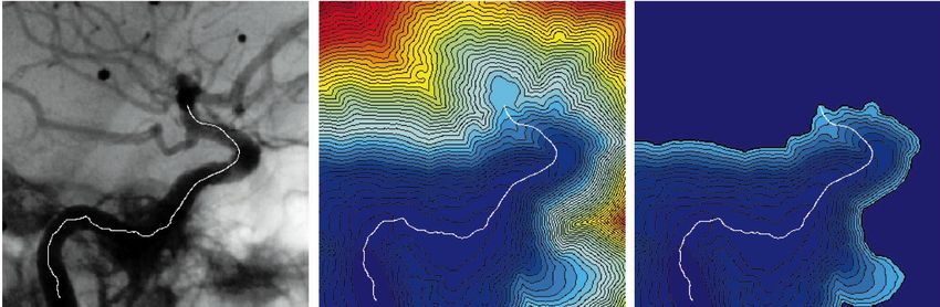
T. Deschamps, L.D. Cohen / Medical Image Analysis 5 (2001) 281 – 299                             283
                                                                                                      →
to lead to different results. In (Cohen and Kimmel, 1997),                solved: (≠C / ≠t) 5 (1 /P˜ )n . It evolves a front starting from
contrary to the classical snake model (but similarly to                   an infinitesimal circle shape around p0 until each point
geodesic active contours), s represents the arc-length                    inside the image domain is assigned a value for U. The
parameter, which means that iC9(s)i 5 1, leading to a new                 value of U( p) is the time t at which the front passes over
energy form. Considering a simplified energy model                        the point p.
without any second derivative term leads to the expression                   The Fast Marching technique, introduced in (Adal-
E(C) 5 ehwiC9i 2 1 P(C)jds. Assuming that iC9(s)i 5 1                     steinsson and Sethian, 1995; Sethian, 1996), and detailed
leads to the formulation                                                  in (Sethian, 1999), was used by Cohen and Kimmel
                                                                          (1996), noticing that the map U satisfies the Eikonal
E(C) 5   E hw 1 P(C(s)) jds.                                    (2)       equation:
         V
                                                                                  ˜
                                                                          i=U i 5 P,                                                  (4)
We now have an expression in which the internal forces
are included in the external potential. In (Cohen and                     Classic finite difference schemes for this equation tend to
Kimmel, 1997), the authors have related this problem with                 overshoot and are unstable. Sethian (1999) has proposed a
the recently introduced paradigm of the level-set formula-                method which relies on a one-sided derivative that looks in
tion. In particular, its Euler equation is equivalent to the              the up-wind direction of the moving front, and thereby
geodesic active contours (Caselles et al., 1997). The                     avoids the over-shooting associated with finite differences:
regularization of this model is now achieved by the
constant w . 0. This term integrates as eV wds 5 w 3                      (maxhu 2 Ui 21, j , u 2 Ui 11, j , 0j)2
                                                                                                                                      (5)
length(C) and allows us to control the smoothness of the                     1 (maxhu 2 Ui, j 21 ,u 2 Ui, j 11 ,0j)2 5 P˜ i,2 j ,
contour (see (Cohen and Kimmel, 1997) for details). We
remove the second order derivatives from the snake term,                  giving the correct viscosity-solution u for Ui, j . The im-
leading to a potential which only depends on the external                 provement made by the Fast Marching is to introduce
forces, and on a regularization term w.                                   order in the selection of the grid points. This order is based
   It makes thus the problem easier to solve, and it is used              on the fact that information is propagating outward,
in minimal paths (Cohen and Kimmel, 1997), active                         because action can only grow due to the quadratic Eq. (5).
contours using level sets (Malladi et al., 1995) and                      Therefore the solution of Eq. (5) depends only on neigh-
geodesic active contours as well (Caselles et al., 1997). In              bors which have smaller values than u.
(Cohen and Kimmel, 1997) and in our Appendix A is also                       The algorithm is detailed in 3D in the next section in
mentioned how the curvature of the minimal path is now                    Table 1. The Fast Marching technique selects at each
controlled by the weight term w. This corresponds to a first              iteration the Trial point with minimum action value. This
order regularization term, and the paths show sometimes                   technique of considering at each step only the necessary
angles. A second order regularization term would give                     set of grid points was originally introduced for the
nicer paths, but this is difficult to include such a term in              construction of minimum length paths in a graph between
the approach.                                                             two given nodes in (Dijkstra, 1959).
   Given a potential P . 0 that takes lower values near                      Thus it needs only one pass over the image. To perform
desired features, we are looking for paths along which the                efficiently these operations in minimum time, the Trial
integral of P˜ 5 P 1 w is minimal. The surface of minimal                 points are stored in a min-heap data-structure (see details
action U is defined as the minimal energy integrated along                in (Sethian, 1999)). Since the complexity of the operation
a path between a starting point p0 and any point p:                       of changing the value of one element of the heap is
                                                                          bounded by a worst-case bottom-to-top proceeding of the
U( p) 5 inf E(C) 5 inf
         !p ,p
           0
                     !p ,p
                       0
                             HEV
                                   ˜
                                   P(C(s))ds
                                            J,                  (3)       tree in O(log 2 N), the total work is about O(N log 2 N) for
                                                                          the Fast Marching on an N points grid. Finding the
                                                                          shortest path between any point p and the starting point p0
where ! p 0 , p is the set of all paths between p0 and p. The             is then simply done by back-propagation on the computed
minimal path between p0 and any point p1 in the image can                 minimal action map. It consists in gradient descent on U
be easily deduced from this action map. Assuming that                     starting from p until p0 is reached, p0 being its global
potential P is always positive, the action map will have                  minimum.
only one local minimum which is the starting point p0 , and
the minimal path will be found by a simple back-propaga-                  2.2. Extension to 3 D minimal paths
tion on the energy map. Thus, contour initialization is
reduced to the selection of the two extremities of the path.                We are interested in this paper in finding a minimal
                                                                          curve in a 3D image. The application that motivates this
2.1.3. Fast marching resolution. In order to compute this                 problem is detailed in Section 5. It can also have many
map U, a front-propagation equation related to Eq. (3) is                 other applications. Our approach is to extend the minimal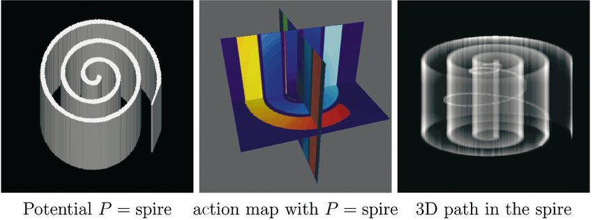
284                                     T. Deschamps, L.D. Cohen / Medical Image Analysis 5 (2001) 281 – 299

Table 1
Fast marching algorithm
? Definition:
   ? Alive is the set of all grid points at which the action value has been reached and will not be changed;
   ? Trial is the set of next grid points (6-connexity neighbors) to be examined and for which an estimate of U has been computed using Eq. (8);
   ? Far is the set of all other grid points, for which there is not yet an estimate for U;
? Initialization:
   ? Alive set is confined to the starting point p0 , with U( p0 ) 5 0;
   ? Trial is confined to the six neighbors p of p0 with initial value U( p) 5 P(    ˜ p);
   ? Far is the set of all other grid points p with U( p) 5 `;
? Loop:
   ? Let (i min , j min , k min ) be the Trial point with the smallest action U;
   ? Move it from the Trial to the Alive set (i.e. Ui min , j min ,k min is frozen);
   ? For each neighbor (i, j, k) (6-connexity in 3D) of (i min , j min , k min ):
     If (i, j, k) is Far, add it to the Trial set and compute U using Table 1;
     If (i, j, k) is Trial, recompute the action Ui, j,k , and update it.

path method of previous section to finding a path C(s) in a                     and used by Cohen and Kimmel (1997) to our 3D
3D image minimizing the energy,                                                 problem.

E P(C(s))ds,
  ˜                                                                  (6)
                                                                                3. Several minimal path extraction techniques
V

where V 5 [0, L], L being the length of the curve. An                              In this section, different minimal path extraction pro-
important advantage of level-set methods is to naturally                        cedures are detailed. We present new back-propagation
extend to 3D. We first extend the Fast Marching method to                       techniques for speeding up extraction, a one end-point path
3D to compute the minimal action U. We then introduce                           extraction method to reduce the need for interaction, and in
different improvements for finding the path of minimal
action between two points in 3D. In the examples that
illustrate the approach, we see various ways of defining the                    Table 2
                                                                                Solving locally the upwind scheme
potential P.
   Similarly to previous section, the minimal action U is                       Algorithm for 3D Up-Wind Scheme
                                                                                1 Considering that we have u > UC 1 > UB 1 > UA 1 , the equation
defined as
                                                                                  derived is

U( p) 5 inf
          !p ,p
            0
                  HE
                   V
                       ˜
                       P(C(s))ds
                                 J
                                 ,                                   (7)
                                                                                                                                  2
                                                                                   (u 2 UA 1 )2 1 (u 2 UB 1 )2 1 (u 2 UC 1 )2 5 P˜ .

                                                                                   Computing the discriminant D1 of Eq. (9) we have two
                                                                                                                                                       (9)

where ! p 0 , p is now the set of all 3D paths between p0 and                      possibilities
p. Given a start point p0 , in order to compute U we start                         ? If D1 $ 0, u should be the largest solution of Eq. (9);
                                                                                     ? If the hypothesis u . UC 1 is wrong, go to 2;
from an initial infinitesimal front around p0 . The 2D                               ? If this value is larger than UC 1 , go to 4;
scheme Eq. (5) is extended to 3D, leading to the scheme                            ? If D1 , 0, at least one of the neighbors A 1 , B1 or C1 has an action
                                                                                     too large to influence the solution. It means that the hypothesis
(maxhu 2 Ui 21, j,k , u 2 Ui 11, j,k , 0j)2                                          u . UC 1 is false. Go to 2;

    1 (maxhu 2 Ui, j 21,k ,u 2 Ui, j 11,k ,0j)2                      (8)        2 Considering that we have u > UB 1 > UA 1 and u , UC 1 , the new
    1 (maxhu 2 Ui, j,k21 , u 2 Ui, j,k 11 , 0j) 5 P˜ i,2 j,k ,
                                                  2                               equation derived is

                                                                                   (u 2 UA 1 )2 1 (u 2 UB 1 )2 5 P 2 .                               (10)
giving the correct viscosity-solution u for Ui, j,k . The
algorithm which gives the order of selection of the points                         Computing the discriminant D2 of Eq. (10) we have two possibilities
in the image is detailed in Table 1.                                               ? If D2 > 0, u should be the largest solution of Eq. (10);
   Considering the neighbors of grid point (i, j, k) in                              ? If the hypothesis u . UB 1 is wrong, go to 3;
6-connexity, we study the solution of the Eq. (8). We note                           ? If this value is larger than UB 1 , go to 4;
                                                                                   ? If D2 , 0, B1 has an action too large to influence the solution.
hA 1 , A 2 j, hB1 , B2 j and hC1 , C2 j the three couples of
                                                                                     It means that u . UB 1 is false. Go to 3;
opposite neighbors such that we get the ordering UA 1 <
UA 2 , UB 1 < UB 2 , UC 1 < UC 2 and UA 1 < UB 1 < UC 1 . To solve              3 Considering that we have u , UB 1 and u > UA 1 , we finally have
the equation, three different cases are to be examined                            u 5 UA 1 1 P. Go to 4;
sequentially in Table 2. We thus extend the Fast Marching
                                                                                4 Return u.
method, introduced in (Adalsteinsson and Sethian, 1995),
T. Deschamps, L.D. Cohen / Medical Image Analysis 5 (2001) 281 – 299 285
Fig. 1. Examples on synthetic potentials.
the next section, a centering path extraction method Runge-Kutta midpoint algorithm or Heun’s method can be
adapted to the problem of tubular structures in images. The used for this path extraction. A simpler descent can be
methods presented in this section are valid in 2D as well as choosing pn 11 5 min hneighbors of pn jU( p), but it gives an
in 3D and this is an important contribution that can be approximated path in the L1 metric. Such a descent has no
useful for image analysis in general, for example in radar more the property of being consistent. As an example, see
applications (Barbaresco and Monnier, 2000), in road in Fig. 3 the computed minimal action map for a 3D
detection (Merlet et al., 1993), or in finding shortest paths potential defined by P(i, j, k) 5 1 ;(i, j, k).
on surfaces (Kimmel et al., 1995). See in Fig. 1-middle the action map corresponding to a
Examples in 2D are used to make the following ideas binarized potential defined by high values in a spiral
easier to understand. We also illustrate the ideas of this rendered in Fig. 1-left. The path found between a point in
section on two synthetic examples of 3D front propagation the center of the spiral and another point outside is shown
in Figs. 1 and 3. Examples of minimal paths in 3D real in Fig. 1-right by transparency.
images are presented for the application described in
Section 5.
The minimal action map U computed according to the 3.1. Partial front propagation
discretization scheme of Eq. (7) is similar to convex, in the
sense that its only local minimum is the global minimum An important issue concerning the back-propagation
found at the front propagation start point p0 where technique is to constrain the computations to the necessary
U( p0 ) 5 0. The gradient of U is orthogonal to the prop- set of pixels for one path construction. Finding several
agating fronts since these are its level sets. Therefore, the paths inside an image from the same seed point is an
minimal action path between any point p and the start interesting task, but in the case we have two fixed
point p0 is found by sliding back the map U until it extremities as input for the path construction, it is not
converges to p0 . It can be done with a simple steepest necessary to propagate the front on all the image domain,
gradient descent, with a predefined descent step, on the thus saving computing time. In Fig. 2 is shown a test on an
minimal action map U, choosing pn 11 5 pn 2 step 3 angiographic image of brain vessels. We can see that there
=U( pn ). More precise gradient descent methods like is no need to propagate further the points examined in Fig.
Fig. 2. Comparing complete front propagation with partial front propagation method on a digital subtracted angiography (DSA) image.286 T. Deschamps, L.D. Cohen / Medical Image Analysis 5 (2001) 281 – 299
2-right, the path found being exactly the same as in Fig.
2-middle where front propagation is done on all the image
domain. We used a potential P(x) 5 u=G *s I(x)u 1 w, where I
is the original image (5123512 pixels, displayed in Fig.
2-left), Gs a Gaussian filter of variance s 5 2, and w 5 1
the weight of the model. In Fig. 2-right, the partial front
propagation has visited less than half the image. This ratio
depends mainly on the length of the path tracked.
3.2. Simultaneous partial front propagation
Fig. 3. 2D and 3D front propagation examples.
The idea is to propagate simultaneously a front from
each end point p0 and p1 . Let us consider the first grid
point p where those front collide. Since during propagation
the action can only grow, propagation can be stopped at
this step. Adjoining the two paths, respectively between p0
and p, and p1 and p, gives an approximation of the exact
minimal action path between p0 and p1 . Since p is a grid
point, the exact minimal path might not go through it, but
in its neighborhood. Basically, it exists a real point p*,
which nearest neighbor on the Cartesian grid is p which
belongs to the minimal path. Therefore, the approximation
done is sub-pixel and there is no need to propagate further.
This colliding fronts method is described in Table 3.
It has two interesting benefits for front propagation:
• It allows a parallel implementation of the algorithm,
dedicating a processor to each propagation;
• It decreases the number of pixels examined during a
partial propagation. With a potential defined by P 5 1,
the action map is the Euclidean distance.
• In 2D (Fig. 3-right), this number is divided by
(2R)2 / 2 3 R 2 5 2;
• In 3D (Fig. 3-left), this number is divided by (2R)3 /
2 3 R 3 5 4.
In Fig. 4 is displayed a test on a digital subtracted Fig. 4. Comparing the partial front propagation with the colliding fronts
method on a DSA image.
angiography (DSA) of brain vessels. The potential used is
P(x) 5 uI(x) 2 Cu 1 w, where I is the original image (256 3
256 pixels, displayed in Fig. 4(a)), C a constant term (mean
value of the start and end points gray levels), and w 5 10 3.3. One end point propagation
the weight of the model. In Fig. 4(b), the partial front
propagation has visited up to 60% of the image. With a We have shown the ability of the front propagation
colliding fronts method, only 30% of the image is visited techniques to compute the minimal path between two fixed
(see Fig. 4(c)), and the difference between both paths found points. In some cases, only one point should be necessary,
is sub-pixel (see Fig. 4(d) where the paths superimposed or the needed user interaction for setting a second point is
on the data do not differ). too tedious in a 3D image. Here we derive a method that
Table 3
Minimal path as intersection of two action maps
Algorithm
? Compute the minimal action maps U0 and U1 to respectively p0 and p1 until they have an Alive point p2 in common;
? Compute the minimal path between p0 and p2 by back-propagation on U0 from p2 ;
? Compute the minimal path between p1 and p by back-propagation on U1 from p2 ;
? Join the two paths found.T. Deschamps, L.D. Cohen / Medical Image Analysis 5 (2001) 281 – 299 287
builds a path given only one end point and a maximum
path length.
As we explain below, we can compute simultaneously at
each point the energy U of the minimal path and its length.
We choose as end point the first point for which the length
of the minimal path has reached a given value. Since the
front propagates faster along lower values of Potential,
interesting paths are longer for a given value of U.
The technique is similar to that of Section 3.1, but the
new condition will be to stop propagation when the first
path corresponding to a chosen Euclidean distance is
extracted. Since the front propagates in a tubular structure,
all the points for which the path length criterion is reached
earlier in the process are located in the same area, far from
the start point. Therefore the first point for which the
length is reached is located in this area and is a valuable
choice as endpoint.
An example of this path length condition is shown on Fig. 6. Problem of path centering.
Fig. 5 which is a DSA image of brain vessels. Propagating
a front with potential P 5 1 computes the Euclidean
distance to the start point. This is obvious from definition
(3), and we can see its illustration with Fig. 3-left. 4. The path centering method
Therefore, we use simultaneously an image-based potential
P1 , for building the minimal path and a potential P2 5 1 for The path is the set of locations that minimize the
computing the path length. integral of the potential in Eq. (2). If the potential is
While we are propagating the front corresponding to P1 constant in some areas, it will lead to the shortest
on the image domain, at each point p examined we Euclidean path. The same thing happens when the po-
compute both minimal actions for P1 (shown in Fig. tential does not vary much inside a tubular shape. The
5-middle) and for P2 (shown in Fig. 5-right). This means minimal path extracted is often tangential to the edges, as
Eq. (5) or Eq. (8) is solved for P2 using the same points shown in Fig. 6, and would not be tuned for a problem
that are used in the scheme for P1 in Table 2. In this case which may require a centered path, like finding the optimal
the action corresponding to P2 is an approximate Eucli- trajectory for virtual endoscopy.
dean length of the minimal path between p and p0 . The general framework for obtaining a centered path is
Although this length is an approximation, it is still a good the following
estimation since it makes use of the same Eikonal equation • Segmentation: the first goal is to obtain the edges of the
scheme. The main advantage of doing so is that it does not tubular region;
add much computation time to the algorithm. • Centered path: once we have this segmented region, we
Note that this Euclidean path length is discontinuous and want to find a path that is as much centered as possible
must be smoothed in order to be used in a robust manner. in it. In order to attract the minimal path to the center of
Fig. 5. Computing the Euclidean path length simultaneously.288 T. Deschamps, L.D. Cohen / Medical Image Analysis 5 (2001) 281 – 299
the region, we use a distance map from the segmented P(i, j) 5 1 for all point (i, j) inside the shape,
edges. P(i, j) 5 infinite for all point (i, j) outside the shape,
In the following we are going to present our method,
U(i, j) 5 0 for all trial point of Section 4.1,
initially presented in (Deschamps et al., 1999) and (De-
U(i, j) 5 infinite elsewhere.
schamps and Cohen, 2000), detailing each step and making
comparisons with other existing techniques. Starting the front propagation from all the points stored in
the min-heap data-structure, we compute the distance map,
4.1. Segmentation step said %, very quickly, visiting only the pixels inside the
tubular object.
In order to find the tubular structure, several approaches Our distance map % is used to create a second potential
can be used. We can use a balloon model (Cohen, 1991) P1 . Choosing a value d to be the minimum acceptable
with a classical snake approach that inflates inside the distance to the walls, we propose the following potential:
object, starting with the given end point. Or we can
P1 (x) 5 max(d 2 % (x); 0)g. (11)
segment the object using its correspondent level-sets
implementation, as in (Malladi et al., 1995) and like the We use it as a potential for a new front propagation
bubbles in (Tek and Kimia, 1995). In fact, this kind of approach: P1 weights the points in order to propagate
region growing method can also be implemented using the faster a new front in the center of the desired regions. This
Fast Marching algorithm. This fast approximation has final propagation produces a path centered inside the
already been used for segmentation in (Malladi and tubular structure in a very fast process.
Sethian, 1998). This allows us to include the segmentation
step in the same framework as our minimal path finding:
4.3. Description of the method
having searched for the minimal action path between two
given points, using a partial front propagation (see Section
The complete method is described in Fig. 7.
3.1), the algorithm provides different sets of points:
• Segmentation: the first step is to compute the weighted
• the points whose action is set and labeled Alive;
distance map given the start and end points. It is
• the points not examined during the propagation and
obtained by front propagation from the start to the end
labeled Far;
point. Notice also that the end point can be determined
• the points at the interface between Alive and Far
automatically by a length criterion as in Section 3.3;
points, whose actions are not set, and labeled Trial.
• Segmentation: the second step is to consider the set of
This last category, the border of the visited points, is a
points which have same minimal action as the endpoint.
contour in 2D and a surface in 3D which defines a
For this, we store the front position (set of trial points)
connected set of pixels or voxels. If the potential is a lot
at the end of the first step.
higher along edges than it is inside the shape, the edges
• Centering Potential: the third step is to compute the
will act as an obstacle to the propagation of the front.
distance map % to the boundary front inside the tubular
Therefore, the front propagation can be used as a seg-
region. For this we propagate inward the front with a
mentation procedure, recovering the object shapes. In this
uniform potential P 5 1. This gives the higher values
case the Trial points define a surface which can be
towards the center of the object.
described as a rough segmentation. Once the front has
• Centered path: the fourth step is to find the minimal
reached the endpoint, we use the front itself to define the
edges.
4.2. Centering the path
Having obtained this interface of Trial points, we now
want the information of distance to the edges. This
information can be either used for a skeletonization,
computing the medial-axis transform, or used as a new
snake energy, that constrains the path in the center of the
tubular shape.
In order to compute this distance, we can use a second
front propagation procedure. The edges ares stored in the
min-heap data-structure (see (Sethian, 1999) for details),
and this is a very fast re-initialization process to compute
this distance. The potential and the initial action for this
second front propagation are defined as follows: Fig. 7. Centering the path inside the object.T. Deschamps, L.D. Cohen / Medical Image Analysis 5 (2001) 281 – 299 289
path between start and end points relatively to the may lead it outside the tubular structure. Also, the un-
distance potential P1 defined in (11) computed from the published work presented by Cuisenaire (1999) details an
previous step. This is obtained by applying again the algorithm which is applied to a tubular object which is
minimal path technique. The front is now pushed to already manually segmented by the user, whereas our
propagate faster in the center of the object. method comprises both steps of segmentation and center-
• Centered path: the final step is to make back-propaga- ing.
tion from the end point using the last minimal action Another category of very similar centered line extraction
map. technique is skeletonization, and particularly the definition
An interesting improvement is that the value of the weight of the medial axis function of Blum (1967) which treats all
w can be automatically set to a very low value: boundary pixels as point sources of a wave front. Consi-
• During the first propagation the regularity of the path is dering that the Fast Marching computes the Euclidean
not important, and w can be very small; distance to an arbitrary set of points using a potential
• During the second propagation, P9 5 P 1 w 5 1; P 5 1, it can also be used for skeletonization.
• During the final propagation the potential based on the However, the purpose of our application is to have a
distance to the object walls is synthetic and leads to smooth line which always stays inside the tubular object
smooth paths even if w < 1. and which is far from the edges. This is motivated by the
As an illustration, a test is proceeded on a DSA image of application to virtual endoscopy (see the next section).
the brain vessels shown in Fig. 8-left. In Fig. 8-center is If one wishes to achieve this task with a skeletonization,
shown the result obtained using a potential based on the like in (Yeorong et al., 1999), he will need and rely on the
image, where the shortest path is tangential to edges. But results of post-processing techniques in order to obtain a
the front propagates only along the vessel direction, and is unique and smooth path inside this segmented object.
rapidly stopped transversally, allowing to compute the Smoothing and removing undesirable small parts of the
distance to the walls. Defining a new potential according to skeleton can be done using techniques shown in (Tek and
Eq. (11) based on this distance map, the second front Kimia, 2001). The main advantage of our approach is that
propagates faster in the center of the vessel. Due to the it gives only one smooth and centered path in a unique and
shape of the iso-action lines of the centered minimal action fast process. Therefore, it cannot be replaced by a simple
shown in Fig. 8-right, the path avoids the edges and medial-axis transform.
remains in the center of the vessel. We will present results In (Paik et al., 1998), the authors extract first the surface
on real 3D data in Section 5.2 applied to the problem of of the colon, then compute a minimal path on this surface
virtual endoscopy (see Fig. 16). and move this initial path to the center of the object by
applying a thinning algorithm to the object segmented and
4.4. Comparison with other work projecting the path on the resulting surface. The algorithm
developed by Kimmel et al. (1998) can be applied to their
Another method to obtain a centered path would be to methods since it computes the minimal path on a surface
make a classical snake minimization on the centering defined by a manifold. Although it seems to produce a
potential P1 , starting from the path obtained previously, smooth centered line, the thinning algorithm is computa-
like it is done in the thesis (Cuisenaire, 1999), a nice tionally inefficient, compared to the speed of our algorithm
application indicated by one of our reviewers. But too that needs less than a minute on a classical inexpensive
much smoothing may lead to a wrong path. For example, computer (300 MHz CPU).
in the case of thin tubular structures, smoothing the path In the different techniques quoted, the main difference
Fig. 8. Comparing classic and centered paths.290 T. Deschamps, L.D. Cohen / Medical Image Analysis 5 (2001) 281 – 299
with our method lies in the fact that the object is manually
segmented by the user. Our method comprises steps of
segmentation and path extraction, and achieves them in a
very fast way. More than a robust and fast method, we
have developed a tool that is used for segmentation,
minimal path tracking, and even potential definition The
main advantage of our approach is that it comprises all
those steps and gives only one smooth and centered path in
a unique and fast process.
Fig. 10. Interior view of a colon, reconstructed from a defined path.
5. Application to virtual endoscopy
modeled using rigid body dynamics; a good example of
In previous sections we have developed a series of
this simulation is presented in (Hong et al., 1997).
issues in front propagation techniques. We study now the
• techniques which focus on the observation of the
particular case of virtual endoscopy, where fast extraction
interior of anatomical objects by extracting trajectories
of centered paths in 3D images with minimum user
inside them, see (Yeorong et al., 1999) for an example.
interactivity is required.
In this article we have decided to focus on the second kind
of techniques. However, the minimal path techniques can
5.1. Targets for virtual endoscopy also be useful for the first kind of methods: Kimmel and
Sethian have applied the Fast-Marching algorithm for a
Visualization of volumetric medical image data plays a robotic application in (Sethian, 1999), for the motion of an
crucial part for diagnosis and therapy planning. The better object with a certain shape and orientation in an image
the anatomy and the pathology are understood, the more with obstacles. They have discretized the Eikonal equation
efficiently one can operate with low risk. Different possi- in a space that describes the object position and orientation
bilities exist for visualizing 3D data: three 2D orthogonal and added a dimension to the problem that could lead to
views (see Fig. 9), maximum intensity projection (MIP, huge computing costs for an interactive 3D application.
and its variants), surface and volume rendering. In par- For the second kinds of virtual endoscopic technique,
ticular, virtual endoscopy allows by means of surface / the system is composed of two parts:
volume rendering techniques to visually inspect regions of 1. A Path construction part, which provides the successive
the body that are dangerous and / or impossible to reach locations of the fly-through in the tubular structure of
physically with a camera (e.g. behind an airway stenosis or interest (see Fig. 10-left);
obstruction, or too small). An extensive definition virtual 2. Three dimensional interior viewing along the endo-
endoscopy can be found in (Jolesz et al., 1997). scopic path. Those views are adjoined creating an
Virtual endoscopy techniques can be divided into two animation which simulates a virtual fly-through through
groups of methods that can collaborate: them (see Fig. 10-right).
• techniques which deal with simulation of a real endo- A major drawback in general remains when the path
scope motion; In this case, virtual endoscopy is very construction is left to the user who manually has to
interactive, simulating the motion of a camera inside the ‘‘guide’’ the virtual endoscope / camera. The required inter-
body, based on an extracted anatomical object that is activity can be very tedious for complex structures such as
Fig. 9. Three orthogonal views of a volumetric CT data set of the colon.T. Deschamps, L.D. Cohen / Medical Image Analysis 5 (2001) 281 – 299 291
orthogonal to the path. If the path is not smooth, the point
of view of the virtual camera will change in an abrupt
manner. There are two ways to achieve this regularization:
• by modifying the view angle of the virtual camera,
being no more orthogonal to the path, but looking in the
direction of a path point which is located far from its
current position (see Fig. 12), or using a running
average of the local direction of the camera;
• by increasing the weight w in Eq. (2) since it has a
smoothing effect on the minimal path (see Appendix A
for details). We preferred to use this technique in the
following examples, since it is efficient and very simple
to add.
We first apply the minimal path construction to the case of
virtual endoscopy in the colon in Section 5.2, then we
extend this technique to other anatomical shapes in Section
5.3.
5.2. Building a potential for virtual colonoscopy
Fig. 11. The complex shape of the colon.
All tests are performed on a volumetric CT scan of size
the colon for example (see Fig. 11). Actually, on most 512 3 512 3 140 voxels, shown in Fig. 9. The grey level
clinical platforms the user must define all path points range is between 0 and 1500. The target is to build a
manually, using for example three 2D orthogonal views, as potential P with the 3D data set allowing paths to stay
shown in Fig. 9, leading to problems as the following: inside the anatomical shapes where end points are located.
• Since the anatomical objects have often complex We thus define the potential by a general model P(x) ˜ 5
a
shapes, they tend to pass in and out of the three uI(x) 2 Imean u 1 w.
orthogonal planes. Consequently the right location is First, the potential must be lower inside the colon in
accomplished by successively entering the projection of order to propagate the front faster, and to avoid problems
the desired point in each of the three planes; with crossing the edges of the anatomical object. In a colon
• The path is approximated between the user defined CT scan, an average position Imean of the colon grey level
points by lines or Bezier splines. If the number of in the histogram can be defined (see Fig. 13) as a peak in
points is not sufficient, it can easily cross an anatomical the histogram where Imean 5200. Secondly, if the path to
wall. be extracted is very long, the situation can lead to
Path construction in 3D images is thus a very critical task pathological cases, and the front can go through potential
and precise anatomical knowledge of the structure is walls. This is frequent for large objects that have complex
needed to set a suitable trajectory, with the minimum
required interactivity.
Numerous techniques try to automate this path construc-
tion process. Most of them use a skeletonization technique,
like in (Yeorong et al., 1999), in order to extract a
centerline in the dataset. But extracting the skeletons of an
anatomical shape requires first to segment it. And the
skeleton often consists in lots of discontinuous trajectories,
and post-processing, as done in (Tek and Kimia, 2001) is
necessary to isolate and smooth the final path. The front
propagation techniques studied in this paper in contrast to
other methods does not require any pre- or post-processing
as explained in Section 4.
It is sometimes necessary to smooth the path extracted
by the front propagation. The point of view in the volume
rendering of the tubular structure is very important,
because it constrains the result of the examination. Thus,
during the virtual fly through, the point of view of the
camera must change smoothly. Traditionally, the position
of the virtual camera frame at a particular path point is Fig. 12. Orientation of the virtual camera.292 T. Deschamps, L.D. Cohen / Medical Image Analysis 5 (2001) 281 – 299
We first need to obtain a shape information. In fact, a CT
scan of the colon contains already a shape information
sufficient to constrain a front propagation. In Fig. 14-left is
shown a slice of a colon volumetric data set. Fig. 14-right
shows the grey level profile along the line drawn in Fig.
14-left. Air fills the colon and is represented in our CT
image by a grey level around 200 (see Fig. 14-right), while
edges are defined by a grey intensity around 1200. Then,
Fig. 13. Localization of the colon in the histogram. ˜ 5 uI(x) 2 I a
using the potential P(x) mean u 1 w, the front
obtained through Fast Marching is stopped by the ana-
shapes and very thin edges, as colon. Then, edges should tomical shapes, as seen in Fig. 15. It illustrates the fact that
be enhanced to enable long trajectories, with a non-linear the Fast Marching can act also as a segmentation tool, as
function. We thus take a 5 2 in order to enhance the noted in Section 4.
dynamic of the image with a quadratic function. In Fig. 16 we show the result of applying this new
However, this potential does not produce paths relevant method to colonoscopy. The edges are obtained via a first
for virtual endoscopy. Indeed, paths should remain not propagation: in Fig. 15 we can see the evolution of the
only in the anatomical object of interest but as far as narrow band during propagation. It gives a rough seg-
possible from its edges. In order to achieve this target, we mentation of the colon and provides a good information
use the centering potential method as detailed in Section 4. and a fast re-initialization technique to compute the
distance to the edges.
Using this distance map as a potential (from Eq. (11))
that indicates the distance to the walls, we can correct the
initial path as shown in Fig. 16-left: the new path remains
more in the middle of the colon. And the value of the
parameter d can be derived from anatomical characteris-
tics. If we know approximately the section of the colon
along the path we can easily choose a value to stay in the
center of the tubular structure.
The two different Figs. 16-middle and 16-right display
Fig. 14. Profile of the colon volume. the view of the interior of the colon from both paths shown
Fig. 15. Propagating inside the colon volume.T. Deschamps, L.D. Cohen / Medical Image Analysis 5 (2001) 281 – 299 293
Fig. 16. Centering the path in the colon.
in Fig. 16-left. With the initial potential, the path is near propagation and choosing the minimal path length (as
the wall, and we see the u-turn, whereas with the new path, explained in Section 3.3). It takes 30 seconds of computing
the view is centered into the colon, giving a more correct time for building the complete path on an Ultra 30 (with
view of the inside of the colon. The new centered path is 300 MHz CPU and 1 Go RAM), comprising steps of
smooth because this final propagation is done on a segmentation of the colon and calculation of the distance
synthetic potential (the distance to the walls) where noise to the walls in order to center the path as detailed in
has been removed. Section 4. The complete virtual fly-through renderings
Therefore, the two end points can be connected correct- (300 images) are computed in approximately 10 minutes
ly, giving a path staying inside the anatomical object. But (the rendering is a tool included in the EasyVision work-
for virtual colonoscopy, it is often not necessary to set the station developed by Philips Medical Systems).
two end points within the anatomical object. The colon
being a closed object with two extremities, we can use the 5.3. Results on Other Anatomical Objects
Euclidean path length stopping criterion as explained in
Section 3.3. Fig. 15 shows the front propagation in the 5.3.1. Trachea CT scan
Fast Marching technique with a starting point belonging to Extracting paths inside the trachea is the same problem
the colon and an Euclidean path length criterion of 500 as in the colon. The dataset used is shown in Fig. 18 by
mm. The image resolution is 1 mm for x and y axes and 4 means of three orthogonal slices of the volume displayed
mm for the z axis. Fig. 17 shows the minimal path together with a path extracted. Air fills the object and give
obtained. Fig. 21 shows rendered views from a few points a shape information all along from throat to lungs.
along the path. Therefore, the anatomical object having a very simple
Interaction is limited to setting the start point for front shape, the path construction with one or two fixed points is
Fig. 17. Views of the minimal path inside the colon volume.294 T. Deschamps, L.D. Cohen / Medical Image Analysis 5 (2001) 281 – 299
Fig. 18. Views of the minimal path inside the trachea.
easier than in the colon case. One example path tracks the tracks the superior sagittal venous canal, using a nonlinear
trachea, using a nonlinear function of the image grey levels function of the image grey levels (P(x)˜ 5 uI(x) 2 100u 2 1
˜ 5 uI(x) 2 200u 2 1 1). Two views of an extracted path
(P(x) 1). Two views of the extracted path in 3D are displayed in
in 3D are displayed in Fig. 18 together with 3 orthogonal Fig. 19 together with 3 orthogonal slices of the dataset. A
slices of the dataset. An endoscopic view along the path is sample of the virtual fly-through along the brain vessel is
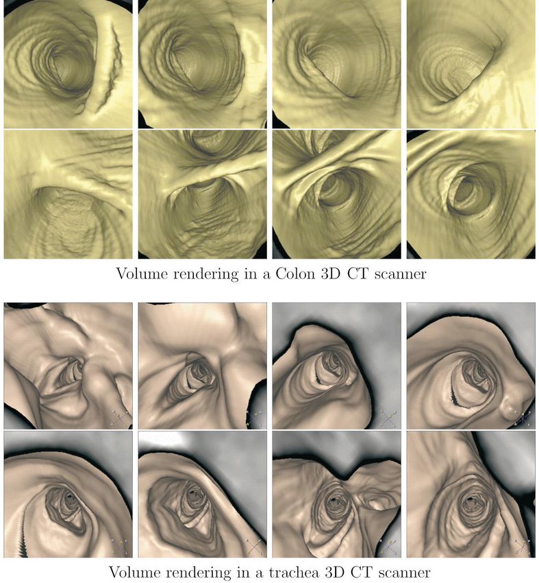
displayed in Fig. 21. displayed in Fig. 22.
5.3.2. Brain magnetic resonance angiography ( MRA)
image 5.3.3. Aorta MR scans
Tests were performed on brain vessels in a MRA scan. A test was made on an aorta MR dataset, shown in Fig.
Three orthogonal slices of this dataset are shown in Fig. 19 20. The propagation measure is based on a nonlinear
together with a path extracted. function of the intensity of the contrast solution that fills
The problem is different, because there is only signal the aorta. This data set is difficult since the intensity of the
from the dye in the cerebral blood vessels. All other contrast product will vary along the aorta (the contrast
structures have been removed. The main difficulty here lies bolus dilutes during the acquisition time). Due to this
in the variations of the dye intensity. The example path non-uniformity, paths can cross other anatomical structures
Fig. 19. Views of the minimal path inside a brain vessel.T. Deschamps, L.D. Cohen / Medical Image Analysis 5 (2001) 281 – 299 295
Fig. 20. Views of the minimal path inside the MR dataset of the aorta.
with similar intensities if the mean value inside the aorta is Philips Medical Systems together with clinicians, and a
not set correctly by the user. paper has been presented in (Truyen et al., 2001).
Our example path tracks one illiaca, using the potential Future works will focus on the definition of potentials
P̃(x) 5 uI(x) 2 1000u 2 1 10 in the MR scan. The dataset for objects with non-uniform grey-level contrast where the
contains noise, and we must use an important weight to success of the tracking approach critically depends on the
smooth the extracted paths. We have displayed a sample of design of the cost function. It will also include the
the endoscopic views of the aorta along the path in Fig. 22. generalization of the path extraction techniques to tubular
anatomical structure with branches, like arterial and bron-
chial trees.
6. Conclusion See also (Cohen, 2001; Cohen and Deschamps, 2001).
In this paper we presented a fast and efficient algorithm
that computes a path useful for guiding endoscopic view-
7. Videos
ing that only depends on a start and end point. This work
was the extension to 3D of a level-set technique developed
Videos of Virtual Endoscopy Fly Through using our
in (Cohen and Kimmel, 1997) for extracting paths in 2D
minimal path technique described in this paper are avail-
images, given only the two extremities of the path and the
able on the following web pages: http: /
image as inputs, with a front propagation equation. We
/ www.ceremade.dauphine.fr / |cohen / MPEG
improved this front propagation method by creating new
It includes the four following sequences:
algorithms which decrease the minimal path extraction
• Aorta Fly Through
computing cost, and reduce user interaction in the case of
• Colon Fly Through
path tracking inside tubular structures. We have proved the
• Brain Fly Through
benefit of our method towards manual path construction,
• Trachea Fly Through
showing that only a few seconds are necessary to build a
complete trajectory inside the body, giving only one or two
end points and the image as input.
Concerning validation of the results, first we have Acknowledgements
noticed the enthusiasm of clinicians who have either seen
demos of our work or have used it. Moreover, we have ´
We thank Drs. Jean-Michel Letang and Sherif Makram-
obtained such good results for very different kinds of Ebeid for fruitful collaborations, and very interesting
medical images. We can assess of the fact that our paths discussions. We thank Jean Pergrale, group leader of the
are acceptable from the good quality of the virtual endo- Medical Imaging Systems Group at Philips Research
scopy video generated. Indeed, our work has been inte- France, for constant support. And we thank Roel Truyen,
grated in the next version of EasyVision Workstation Dr. Bert Verdonck and all the MIMIT team of Dr. Frans
delivered by Philips Medical Systems. A more thorough Gerritsen at Philips Medical Systems, The Netherlands, for
systematic validation has been made with colleagues at providing datasets and helpful ideas on the subject.296 T. Deschamps, L.D. Cohen / Medical Image Analysis 5 (2001) 281 – 299
Fig. 21. Virtual endoscopy in the colon and in the trachea.
Appendix A. Paths of minimal action propagating in every direction at the same speed. The
corresponding iso-action lines are circles, and their radius
We give here some remarks and comments on the is the Euclidean distance to the start point. The minimal
minimal path approach described in Section 2 and intro- paths are straight lines.
duced for 2D in (Cohen and Kimmel, 1997). The potential is multi-valued in Fig. 23(b), the higher
value being the upper-half part of the image. One can
A.1. Understanding the role of the potential map easily see that the front propagation speed is quicker in the
The aim of the potential used in Eq. (4) is to propagate lower half part, because the space between the iso-action
the front in the desired regions, in order to extract a lines (level sets of the surface) is bigger. The minimal
minimal path corresponding to the wanted features. paths are piecewise linear.
In Fig. 23(a) one can see the iso-action lines of the This is similar to Fermat’s principle on the minimality
surface of minimal action provided by a front propagation of the light path: we can observe on Fig. 23(a) that paths
on a univalued potential. Visualization is focused on the are straight lines in homogeneous media, and that paths are
lines of iso-action. Without any obstacle, the front is deviated at the junction between two different homoge-T. Deschamps, L.D. Cohen / Medical Image Analysis 5 (2001) 281 – 299 297
Fig. 22. Virtual endoscopy in the brain vessels and in the aorta.
neous media on Fig. 23(b). The path joining the point in A.2. The regularity of the path
the middle right corresponds to the well-known mirage In (Cohen and Kimmel, 1997), it is proven that weight
effect. w in Eq. (2) can influence curvature and be used as a
smoothing term. An upper bound for the curvature mag-
nitude uk u along the minimal path is found, ( being the
image domain:
sup ( i=Pi
uk u < ]]]. (A.1)
w
A.2.1. Influence on the gradient descent scheme. The
exact minimal path is obtained with a gradient descent. But
care must be paid on the choice of the gradient step to
avoid oscillations.
If the weight w is set to a small value e the extracted
Fig. 23. Propagation and minimal paths on synthetic cases. path length is not limited at all, nor the curvature mag-298 T. Deschamps, L.D. Cohen / Medical Image Analysis 5 (2001) 281 – 299
nitude in Eq. (A.1). Therefore in zones where the action
map is flattened, the slope being as small as e, the path can
have a spaghetti-like trajectory. The minimal path being
obtained by steepest gradient descent, directions are evalu-
ated by interpolation based on nearest neighbors on the
Cartesian grid. If the discrete gradient step Dx is too large,
the approximation of this trajectory will produce oscilla-
tions between relative positions. Those oscillations can
lead to a huge number of path points larger than forecasted
allocations.
We have made a test on a region of the data shown in
Fig. 24-left where the steepest gradient fails (with a Fig. 25. Smoothing the minimal path with the weight w: the paths with
number of path points limited). The cost map when w 1 5 1 and w 2 5 20.
tracking a vessel is displayed in Fig. 24-middle. Taking
w 5 0.1 leads to a curvature magnitude k < 10 3 . The
steepest gradient scheme oscillates, for a given step size,
and stops as shown in Fig. 24-right. Therefore, increasing
w maintains a lower upper-bound on the curvature mag-
nitude and makes the steepest gradient descent scheme
robust. Another method is to use more robust gradient
descent techniques like Runge-Kutta where the step size of
the gradient descent can be locally adapted.
A.2.2. Influence on the number of points visited. This
section illustrates the influence of the weight w of Eq. (2) Fig. 26. Smoothing the minimal path with the weight w: the action maps.
on the necessary number of voxels visited for a path
extraction. In Figs. 25 is shown the tracking of a vessel in
a X-Ray image of the femoral vessels, using different because the tune of w smoothes the image, as it reduces
weights w 1 5 1 and w 2 5 20. The smoothing done by the upper-bound on curvature magnitude in Eq. (A.1).
increasing the weight can be observed in a zoom on the For the virtual endoscopy application, the centering
paths shown in Fig. 25-right. We can also observe the potential relies on the segmentation step described on page
influence of increasing the weight in Fig. 26 where each 3. Path sensitivity to the noise in the data is not important
path is displayed superimposed on its respective action during this step, and we take w < 1 in order to extract a
map. For a small weight w 1 5 1, the path is not smoothed, set of voxels which is a rough segmentation of our tubular
as shown in Fig. 26-left. For a weight w 2 5 20, leading to object.
the inequality uk2 u < 0.75, the path is smooth. Differences The path extraction is finally done using a synthetic
appear also in the sets of points visited during propaga- potential representing a function of the distance to the
tions: it is smaller with weight w 1 5 1. It means that object shape, where initial noise has disappeared. There-
propagation is quicker for small weights. It propagates in fore, taking w as small as possible will not lead to a path
every directions for a higher weight (see Fig. 26-right), that oscillates inside the virtual fly through.
Fig. 24. Failure of the steepest gradient descent on a bolus chase reconstruction data.You can also read