Efficient Actor-Critic Reinforcement Learning With Embodiment of Muscle Tone for Posture Stabilization of the Human Arm - MIT Press
←
→
Page content transcription
If your browser does not render page correctly, please read the page content below
LETTER                                                       Communicated by Hiroyuki Kambara

                   Efficient Actor-Critic Reinforcement Learning
                   With Embodiment of Muscle Tone for Posture
                   Stabilization of the Human Arm

                   Masami Iwamoto
                   iwamoto@mosk.tytlabs.co.jp
                   Daichi Kato
                   d-kato@mosk.tytlabs.co.jp
                   Toyota Central R&D Labs., Aichi 480-1192 Japan

                   This letter proposes a new idea to improve learning efficiency in rein-
                   forcement learning (RL) with the actor-critic method used as a muscle
                   controller for posture stabilization of the human arm. Actor-critic RL
                   (ACRL) is used for simulations to realize posture controls in humans or
                   robots using muscle tension control. However, it requires very high com-
                   putational costs to acquire a better muscle control policy for desirable
                   postures. For efficient ACRL, we focused on embodiment that is sup-
                   posed to potentially achieve efficient controls in research fields of artifi-
                   cial intelligence or robotics. According to the neurophysiology of motion
                   control obtained from experimental studies using animals or humans, the
                   pedunculopontine tegmental nucleus (PPTn) induces muscle tone sup-
                   pression, and the midbrain locomotor region (MLR) induces muscle tone
                   promotion. PPTn and MLR modulate the activation levels of mutually
                   antagonizing muscles such as flexors and extensors in a process through
                   which control signals are translated from the substantia nigra reticulata to
                   the brain stem. Therefore, we hypothesized that the PPTn and MLR could
                   control muscle tone, that is, the maximum values of activation levels of
                   mutually antagonizing muscles using different sigmoidal functions for
                   each muscle; then we introduced antagonism function models (AFMs) of
                   PPTn and MLR for individual muscles, incorporating the hypothesis into
                   the process to determine the activation level of each muscle based on the
                   output of the actor in ACRL.
                      ACRL with AFMs representing the embodiment of muscle tone suc-
                   cessfully achieved posture stabilization in five joint motions of the right
                   arm of a human adult male under gravity in predetermined target angles
                   at an earlier period of learning than the learning methods without AFMs.
                   The results obtained from this study suggest that the introduction of em-
                   bodiment of muscle tone can enhance learning efficiency in posture sta-
                   bilization disorders of humans or humanoid robots.

                   Neural Computation 33, 129–156 (2021)                © 2020 Massachusetts Institute of Technology
                   https://doi.org/10.1162/neco_a_01333

Downloaded from http://www.mitpressjournals.org/doi/pdf/10.1162/neco_a_01333 by guest on 16 March 2021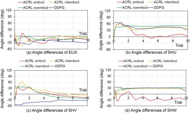
130                                                                       M. Iwamoto and D. Kato

                    1 Introduction

                    Humans exist in an environment controlled by gravity. Without muscle ac-
                    tivity, we cannot stand or perform activities of daily living. How humans
                    control their muscles for posture stabilization and intentional motions is
                    one of the major questions in neurology and robotics. In particular, pos-
                    ture stabilization is critical for understanding the mechanisms of human
                    motions, because human motions start from a determined posture that is
                    stabilized in a gravity-controlled environment. Many researchers have ex-
                    erted valuable efforts to understand how multiple muscles are controlled
                    to realize target postures or target motions. The linear feedback gain con-
                    trol method, such as the proportional integral derivative control law, and
                    optimal control algorithms with cost functions were applied to estimate the
                    activation levels of several muscles for posture stabilization and intentional
                    motions (Rooij, 2011; Kato, Nakahira, Atsumi, & Iwamoto, 2018; Thelen,
                    Anderson, & Delp, 2003). These methods are useful to estimate the acti-
                    vation of multiple muscles in order to hold a target posture, reach a final
                    goal, or follow a predetermined path under a given dynamic environment.
                    For these reasons, these methods cannot be used to achieve robust motion
                    control under unexpected dynamic environments, different from a given
                    dynamic environment.
                       Reinforcement learning (RL) has recently become attractive as a method
                    that performs action selection by interacting with unknown environments.
                    Among the many methods in RL, the actor-critic model (Barto, 1995), which
                    is presumed to reflect RL in the basal ganglia (Barto, 1995; Doya, 2000b;
                    Morimoto & Doya, 2005), has been used to realize target postures or target
                    motions in expected or unexpected dynamic environments (Kambara, Kim,
                    Sato, & Koike, 2004; Kambara, Kim, Shin, Sato, & Koike, 2009; Iwamoto,
                    Nakahira, Kimpara, Sugiyama, & Min, 2012; Min, Iwamoto, Kakei, & Kim-
                    para, 2018). Kambara et al. (2004) proposed a computational model of
                    feedback-error-learning with actor-critic RL (ACRL) for arm posture control
                    and learning. Their model realized posture stabilization of a human hand
                    after learning from 22,500 trials (each trial continues up to 2 s), but they
                    used a two-link arm model of two joints and six muscles, and no gravity
                    effect was implemented, which enabled easier simulation of realistic mo-
                    tions of the human arm with multiple muscles under dynamic environ-
                    ments, including an environment controlled by gravity. By contrast, Min
                    et al. (2018) proposed a musculoskeletal finite element (FE) model of the
                    human right upper extremity and a muscle control system that consists of
                    ACRL and muscle synergy control strategy. They successfully reproduced
                    arm posture stabilization in unexpected dynamic environments in which
                    a weight was suddenly loaded on the hand under gravity after learning
                    from approximately 700 trials (each trial continued for 2 s). However, be-
                    cause the FE model contained the elastic part of each muscle, including
                    multiple nodes of 6 degrees of freedom and contact definitions between

Downloaded from http://www.mitpressjournals.org/doi/pdf/10.1162/neco_a_01333 by guest on 16 March 2021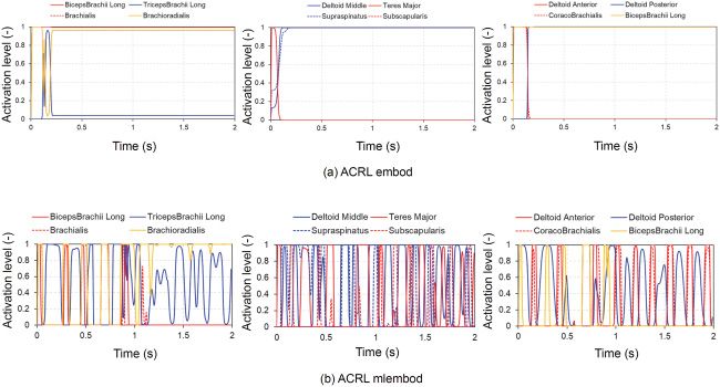
ACRL With Embodiment for Arm Stabilization                                            131

                   muscles and rigid wrapping shell elements implemented due to reproduc-
                   tion of the muscular action line, iterative calculation of learning took time.
                   In these previous studies on ACRL, very high computational costs, de-
                   pending on the biofidelity of the human arm model, were needed to ob-
                   tain simulation results, including those for muscle control strategies for arm
                   posture stabilization. Although ACRL can be used for posture stabilization
                   of computational human body models with multiple muscles or humanoid
                   robots including muscular structures, especially for posture stabilization of
                   a humanoid robot, efficient ACRL is critical to achieve high performance in
                   robots with motion controls with an online learning process.
                      Some studies have recently been conducted to reduce computational
                   costs in RL (Silver et al., 2014; Popov et al., 2018; Andrychowicz et al., 2017).
                   Silver et al. (2014) proposed a deep deterministic policy gradient algorithm
                   (DDPG) for efficient ACRL with continuous actions and applied it to an oc-
                   topus arm task, the goal of which was to strike a target with any part of the
                   arm consisting of six segments and attached to a rotating base. DDPG suc-
                   cessfully realized efficient learning with 50 continuous state variables and
                   20 action variables and controlled three muscles in each segment, as well
                   as rotations of the base. Popov et al. (2018) used DDPG with a model-free
                   Q-learning-based method to design reward function and realized dexter-
                   ous manipulations of robot hands with a small number of trials as intended
                   by designers. Andrychowicz et al. (2017) proposed DDPG with a method
                   called hindsight experience replay that increases teaching signal using fail-
                   ure experiences for learning and then achieved complicated behaviors of a
                   robot arm in a small number of trials. In these previous studies (Popov et al.,
                   2018; Andrychowicz et al., 2017), robot arms with 7 or 9 degrees of freedom
                   were used for manipulating objects in the MuJoCo physics engine (Todorov,
                   Erez, & Tassa, 2012), for example, picking up a ball or a Lego brick and
                   moving it to a goal position. Although the controllers using RL and an oc-
                   topus arm or robot arms interacted in a dynamic environment, the method-
                   ology to realize efficient learning was focused on the internal control sys-
                   tem with RL, corresponding to the brain. By contrast, there is increasing
                   interest in the effects of embodiment on intelligent behavior and cognition
                   (Pfeifer, Lungarella, & Iida, 2007; Hoffmann & Pfeifer, 2012). Hoffmann and
                   Pfeifer (2012) argued that embodiment can improve the cognitive functions
                   of artificial intelligence. For example, passive dynamic walkers are capable
                   of walking down an incline path without any actuation and without con-
                   trol. Without any motors and any sensors, the walker with mainly leg seg-
                   ment lengths, mass distribution, and foot shape can realize walking with the
                   influence of gravity as the only power source. This indicates that embodi-
                   ment can achieve efficient control of walking or balancing in dynamic en-
                   vironments. Therefore, to identify an efficient RL method for human arm
                   posture stabilization under gravity, we developed an ACRL model to the
                   control activation of multiple muscles for human arm posture stabilization
                   under gravity, in which we introduced a musculoskeletal model of a human

Downloaded from http://www.mitpressjournals.org/doi/pdf/10.1162/neco_a_01333 by guest on 16 March 2021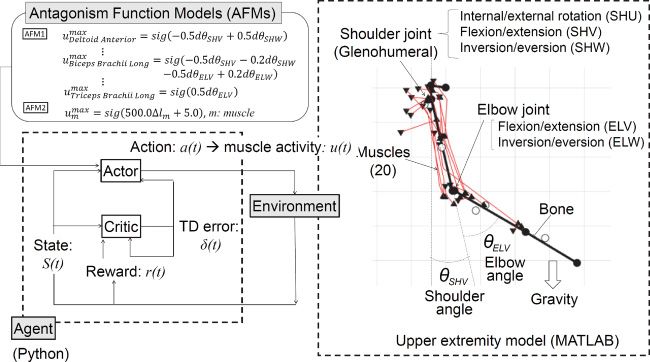
132                                                                       M. Iwamoto and D. Kato

                    Figure 1: Architecture of actor-critic reinforcement learning (ACRL).

                    upper extremity and antagonism function models (AFMs) for embodiment
                    to achieve efficient learning for human arm posture stabilization.

                    2 Method

                    In a previous study, Min et al. (2018) developed a muscle control system that
                    consisted of ACRL and muscle synergy control strategy and reproduced
                    arm posture stabilization using a musculoskeletal FE model. In this study,
                    we also used ACRL for posture stabilization of a computational human arm
                    model under gravity. Figure 1 shows the architecture of ACRL and a mus-
                    culoskeletal model of the human right upper extremity used in this study.

                        2.1 Musculoskeletal Model of the Human Right Upper Extremity. In
                    this study, we developed a musculoskeletal model of the right upper ex-
                    tremity of a human adult male using Matlab (MathWorks, U.S.A.) as shown
                    on the right side of Figure 1. The skeletal parts of the upper extremity
                    model were divided into five parts—the scapula, humerus, ulna, radius,
                    and hand—which were modeled using rigid bodies. The inertia properties
                    of Ixx , Iyy , and Izz and masses of rigid bodies simulating skeletal parts of the
                    upper extremity model are listed in Table 1. These data were obtained from
                    an FE model of the human body that we developed previously (Iwamoto
                    et al., 2012). Inertia properties of Ixy , Iyz , and Izx were set to 0.0 for all rigid
                    bodies. The elbow joint was modeled using a mechanical joint that can rep-
                    resent two elbow joint motions, namely, flexion-extension and inversion-
                    eversion, whereas the shoulder joint was modeled using the same kind of
                    mechanical joint that can represent three shoulder joint motions, namely,

Downloaded from http://www.mitpressjournals.org/doi/pdf/10.1162/neco_a_01333 by guest on 16 March 2021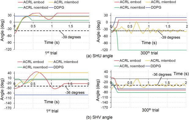
ACRL With Embodiment for Arm Stabilization                                                    133

                   Table 1: Inertia Properties and Masses of Rigid Bodies Simulating Skeletal Parts
                   of the Human Right Arm Used in This Study.

                                                          Ixx             Iyy               Izz          Mass
                                    Rigid Body         [kg∗mm2 ]       [kg∗mm2 ]        [kg∗mm2 ]        [kg]
                                    Scapula               3.432            4.166            5.097        1.27
                                    Humerus               2.496           16.393           17.228        1.69
                                    Ulna                  0.028            0.628            0.639        0.14
                                    Radius                0.598            2.625            2.722        0.65
                                    Hand                  0.575            1.206            1.351        0.54

                                    Source: Iwamoto et al. (2012).

                   internal-external rotation, flexion-extension, and inversion-eversion. The
                   musculoskeletal model has 20 muscles: deltoid anterior, deltoid middle,
                   deltoid posterior, teres major, teres minor, supraspinatus, infraspinatus,
                   subscapularis, coraco brachialis, biceps brachii (long head and short head),
                   triceps brachii (long head, lateral head, medial head), brachialis, brachio-
                   radialis, pronator teres, anconeus, supinator, and pronator quadratus. Each
                   muscle was modeled using the Hill-type muscle model that includes a con-
                   tractile element and a parallel elastic element according to Zajac (1989). The
                   muscle activation level u was associated with the muscular force of a muscle
                   m, fm using the following equation:

                             fm = fmax (u fL fV + fPE ) cos α,                                                  (2.1)
                                        ¯
                                            (lm − 1)2
                              fL = exp −                 ,                                                      (2.2)
                                                SL
                                   ⎧
                                   ⎪
                                   ⎪ 0                                    (v̄ m < −1),
                                   ⎪
                                   ⎪
                                   ⎪
                                   ⎪
                                   ⎨ 1 + v̄ m                             (−1 ≤ v̄ m < 0),
                             fV = 1 − v̄ m /A f                                                                 (2.3)
                                   ⎪
                                   ⎪
                                   ⎪
                                   ⎪ (B f − 1) + v̄ m (2 + 2/A f )B f
                                   ⎪
                                   ⎪
                                   ⎩                                      (0 ≤ v̄ m ),
                                       (B f − 1) + v̄ m (2 + 2/A f )
                                   ⎧
                                   ⎪
                                   ⎨0                                (l¯m < 1),
                            fPE = exp(kPE (l¯m − 1)/e0 ) − 1                                                    (2.4)
                                   ⎪
                                   ⎩                                 (1 ≤ l¯m )
                                            exp(kPE ) − 1

                   where l¯m = lm /lm0 , v̄ m = l˙m /v max are the normalized length and normal-
                   ized contractile velocity of a muscle m, respectively. Parameters of
                   SL , A f , B f , kPE , and e0 were determined as SL = 0.45, A f = 0.25, B f =
                   1.4, kPE = 5.00, and e0 = 0.60 based on Thelen (2003). fmax (N), α (deg), lm0
                   (m), and v max (m/s) are the maximum contractile force, pennation angle,

Downloaded from http://www.mitpressjournals.org/doi/pdf/10.1162/neco_a_01333 by guest on 16 March 2021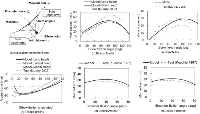
134                                                                       M. Iwamoto and D. Kato

                    Table 2: Parameters of Human Arm Musculoskeletal Model Used in This Study.

                                                              PCSA        Pennation Angle          Optimal Fiber Length
                       Muscle                                 [mm2 ]           [deg]                      [mm]
                       Deltoid anterior                        546                22.0                    193.5
                       Deltoid middle                         1000                15.0                    165.1
                       Deltoid posterior                       469                18.0                    190.5
                       Teres major                             497                16.0                    121.9
                       Teres minor                             244                24.0                    104.1
                       Supraspinatus                           770                 9.0                    120.0
                       Infraspinatus                          1200                11.5                    135.0
                       Subscapularis                          2000                12.9                    126.0
                       Coraco brachialis                       167                27.0                    185.4
                       Biceps brachii long head                413                 0.0                    270.0
                       Biceps brachii short head               396                 2.5                    230.0
                       Triceps brachii long head               800                10.0                    312.4
                       Triceps brachii lateral head           1050                10.0                    246.4
                       Triceps brachii medial head             610                17.0                    213.4
                       Brachialis                              948                 4.0                    199.0
                       Brachioradialis                         293                 2.0                    250.0
                       Pronator teres                          437                10.0                    160.0
                       Anconeus                                200                 0.0                     58.0
                       Supinator                               395                 0.0                     57.0
                       Pronator quadratus                      260                10.0                     39.3

                       Source: Winters (1990); Murray et al. (2000).

                    optimal fiber length, and maximum contractile velocity, respectively. fmax
                    was determined by fmax = σm kg. σm represents the physiological cross-
                    sectional area (PCSA) of a muscle m, a coefficient k = 5.5 (kg/cm2 ) accord-
                    ing to Gans (1982), and g = 9.8 (m/s2 ) of gravitational acceleration. v max
                    was determined by v max = 10lm0 according to Thelen (2003). The PCSA of
                    each muscle was determined based on the study by Winters (1990). α and
                    lm0 were determined based on the methods of Murray, Buchanan, and Delp
                    (2000). Parameters of PCSA, pennation angle, and optimal fiber length used
                    in the musculoskeletal model of human arm are listed in Table 2.
                       The moment arm of a muscle was determined by the muscle’s line of ac-
                    tion for the joint position and represents the relationship between muscular
                    force and joint motion. The biofidelity of the musculoskeletal model was
                    validated by comparisons between the moment arm of each muscle pre-
                    dicted by the model and that obtained from experimental test data using
                    human subjects. In this study, we created the lines of action of the 20 mus-
                    cles by referring to the surface data of the muscles obtained from anatomi-
                    cal models of ZygoteBody (Zygote Media Group, U.S.A.). The moment arm
                    vector of a muscle m was defined as a normal vector from the center of the
                    elbow or shoulder joint to the line of action of the muscular force using rm
                    as shown in Figure 2a, and the moment around the elbow or shoulder joint

Downloaded from http://www.mitpressjournals.org/doi/pdf/10.1162/neco_a_01333 by guest on 16 March 2021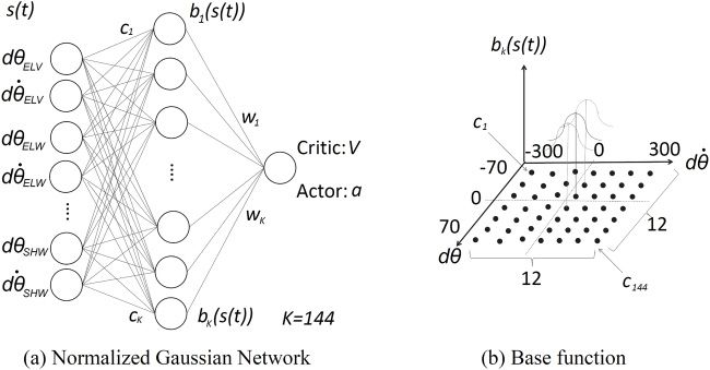
ACRL With Embodiment for Arm Stabilization                                             135

                   Figure 2: Comparisons of moment arm versus elbow or shoulder flexion angles
                   between model prediction and test data.

                   τ was calculated using the contractile force of a muscle m, fm , as follows:

                            τ = rm × f m ,                                                               (2.5)

                   where × represents the outer product of the vectors. According to the prin-
                   ciple of virtual work, the moment arm |rm | can be calculated using the fol-
                   lowing equation:

                            |rm | = lm /θ ,                                                            (2.6)

                   where θ is the differential of joint angle θ and lm is the differential of
                   muscle length.
                       In this study, the moment arms of 17 muscles-deltoid anterior, del-
                   toid middle, deltoid posterior, teres major, teres minor, supraspinatus,
                   infraspinatus, subscapularis, biceps brachii (long head and short head),
                   triceps brachii (long head, lateral head, medial head), brachialis, brachio-
                   radialis, pronator teres, and anconeus—were validated against the exper-
                   imental test data obtained from Kuechle, Newman, Itoi, Morrey, and An
                   (1997, 2000); Amis, Dowson, and Wright (1979); An, Hui, Morrey, Lin-
                   scheid, and Chao (1981); Murray, Delp, and Buchanan (1995); and Mur-
                   ray, Buchanan, and Delp (2002), and the predicted moment arms of each
                   muscle agreed with the test data. In this paper, validation results for only
                   the muscles related to flexion-extensions of the elbow and shoulder joints
                   are shown. Figures 2b to 2d show comparisons of the moment arm-elbow

Downloaded from http://www.mitpressjournals.org/doi/pdf/10.1162/neco_a_01333 by guest on 16 March 2021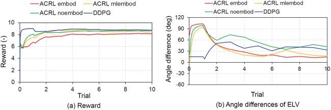
136                                                                       M. Iwamoto and D. Kato

                    flexion angle relationship between model prediction using equation 2.6 and
                    experimental test data obtained from Murray et al. (2002). Figures 2b to 2d
                    show the results of the biceps brachii (long head and short head), brachialis,
                    and triceps brachii (long head, lateral head, and medial head), respectively.
                    Figures 2e and 2f show comparisons of the moment arm-shoulder flexion
                    angle relationship between model prediction data using equation 2.6 and
                    experimental test data obtained from Kuechle et al. (1997). These figures in-
                    dicate that a moment arm of each muscle predicted by the developed mus-
                    culoskeletal model almost fell within the test data corridor or almost agreed
                    with the test data. This suggests that the developed musculoskeletal model
                    has good biofidelity to simulate the elbow or shoulder joint motion with
                    muscle activity.
                       The elbow and shoulder joint motions can be calculated using a for-
                    ward dynamic method that solves an equation of motion in the muscu-
                    loskeletal model representing the following differential algebraic equation
                    (Nikravesh, 1988)
                            ⎡                   ⎤⎡ ⎤ ⎡                            ⎤
                                M     PT     BT     q̈            g−b
                            ⎢                   ⎥⎢ ⎥ ⎢               ˙ − β ∗2  , ⎥
                            ⎣P         0      0 ⎦ ⎣ σ ⎦ = ⎣ c − 2α ∗             ⎦                            (2.7)
                                B      0      0     λ                ˙
                                                             γ − 2α  − β 2

                    where q̈ is the generalized acceleration and the generalized coordinate of
                    the rigid body i is represented by qi = [xTi pTi ]T (T:Transpose) including a
                    coordinate system of each rigid body position xi that has principal axes of
                    the inertia as coordinate axes, a center of gravity of each rigid body as an
                    origin of the coordinate, and a posture expression pi using Euler parame-
                    ters that represent rotating postures with four variables (Nikravesh, 1988).
                    M is an inertia matrix based on the inertial property of rigid bodies repre-
                    senting skeletal parts. g represents generalized forces including muscular
                    forces obtained from equation 2.1 of each muscle m and gravity force calcu-
                    lated as gravitational acceleration multiplied by a mass of each rigid body.
                    b indicates centrifugal forces and Coriolis forces. P and c are a coefficient
                    matrix and a constant term obtained by second-order time derivatives of
                    constraint conditions of Euler parameters, respectively, whereas B and γ
                    are a coefficient matrix and a constant term obtained by second-order time
                    derivatives of constraint conditions based on the joint location and its de-
                    gree of freedom, respectively. σ and λ are Lagrange multipliers.  and          ˙
                    are constraint conditions of Euler parameters and velocity constraint con-
                    ditions by its time derivative, respectively, while  and        ˙ are constraint
                    conditions of the joint and its velocity constraint conditions, respectively.
                    α ∗ , β ∗ , α, and β are weight coefficients adjusting the specific weight of each
                    constraint condition.
                         In the forward dynamic calculation, coefficient matrices, P and B, on the
                    left side of equation 2.7 and constant terms, c and γ, on the right side of

Downloaded from http://www.mitpressjournals.org/doi/pdf/10.1162/neco_a_01333 by guest on 16 March 2021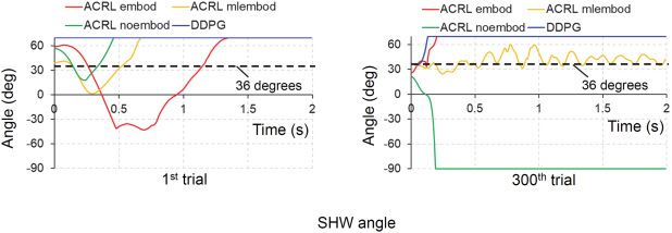
ACRL With Embodiment for Arm Stabilization                                            137

                   Figure 3: Normalized gaussian network and base function.

                   the equation are calculated using the generalized coordinate and velocity,
                   qt , q̇t at each input time t for each muscular force and gravity force of each
                   rigid body, with reference to the study of Nikravesh (1988). Then the gener-
                   alized acceleration q̈t is obtained by solving equation 2.7 using the mldivide
                   function of Matlab. The elbow joint motion can be obtained by calculating
                   the generalized velocity and coordinate, q̇t+t , qt+t sequentially at the next
                   time t + t using a solver of the ordinary differential equation of Matlab,
                   ode113. In the simulation, initial values of the generalized coordinate are
                   given by inputting the joint angle at the initial time, and the initial value
                   of the generalized velocity is given as zero in case of a static situation. The
                   joint angle is obtained as a Euler angle by calculating a homogeneous trans-
                   formation matrix of the generalized coordinates qt of two rigid bodies con-
                   nected via the joint.

                       2.2 ACRL Method. In this study, we implemented ACRL, one of the
                   methods using temporal difference (TD) learning, to acquire a muscle con-
                   trol policy for posture stabilization under unknown environments. A con-
                   trol network, called actor, and an evaluation network, called critic, are used
                   in the actor-critic method as shown in Figure 1. Each network is constructed
                   using a three-layer neural network including the input layer that consists
                   of a state variable s(t) as shown in Figure 3a. The critic network predicts
                   value function V (s(t)), and the actor network acquires control policy a(t)
                   that maximizes the value function V (s(t)) through learning trials using the
                   critic and actor networks, respectively. In this study, the critic and actor net-
                   works were implemented using the normalized gaussian network (NGnet)
                   and a continuous-time formulation of RL (Doya, 2000a) because we target
                   posture stabilization of the human arm with multidimensional degrees of

Downloaded from http://www.mitpressjournals.org/doi/pdf/10.1162/neco_a_01333 by guest on 16 March 2021
138 M. Iwamoto and D. Kato
freedom, and the state variable s(t) should be defined in continuous and
multidimensional state spaces. In the NGnet, the continuous state space
was modeled using the gaussian soft-max network that can generalize the
state space by extrapolation even out of range in a base function of the radial
basis function network (Shibata & Ito, 1999).
We set the 10 state spaces using the difference dθ (t) between current
angle θ (t) and target angle θtrg and the difference dθ˙ (t) between current
angular velocity θ˙ (t) and target angular velocity θ˙trg as s(t) = (dθELV (t),
dθ˙ELV (t), dθELW (t), dθ˙ELW (t), dθSHU (t), dθ˙SHU (t), dθSHV (t), dθ˙SHV (t), dθSHW (t),
dθ˙SHW (t)). ELV, ELW, SHU, SHV, and SHW represent flexion-extension of
the elbow joint, inversion-eversion of the elbow joint, internal-external
rotation of the shoulder joint, flexion-extension of the shoulder joint,
and inversion-eversion of the shoulder joint, respectively. According to
anatomical text (Neumann, 2010), angle ranges of ELV, ELW, SHU, SHV,
and SHW were set from −135 to 17 degrees, from 0 to 180 degrees, from
−120 to 40 degrees, from −170 to 50 degrees, and from −90 to 70 degrees,
respectively. Using NGnet, the state value function V (s(t)) in the critic
and the action value function am (s(t)) for the mth muscle in the actor are
represented as follows:
K
V (s(t)) = wV
k bk (s(t)), (2.8)
k=1
K
am (s(t)) = wka bk (s(t)), (2.9)
k=1
where bk (s(t)) denotes base function and is represented by the following
equations:
⎡ 2 ⎤
Bk (s(t)) n
s (t) − c
, Bk (s(t)) = exp ⎣− ⎦ , (2.10)
i i
bk (s(t)) = K
l=1 Bl (s(t)) i=1
σbi
where ci denotes the coordinates (dθ , dθ˙ ) of the center of activation function,
and σbi , K, and n represent a constant, the number of base functions, and the
number of states s(t), respectively.
In this study, we treated five joint motions of the human arm, including
elbow joint motions with 2 degrees of freedom and shoulder joint motions
with 3 degrees of freedom and set the neutral angles of ELV, ELW, SHU,
SHV, and SHW to −58, 54, −39, −36, and 36 degrees, respectively by re-
ferring to space attitude reported by NASA (Tengwall et al., 1982), because
each muscle is supposed to have its equilibrium length in the space atti-
tude. However, because the musculoskeletal model had −30 degrees of the
ELV angle initially, the neutral angle of ELV was modified to −88 degrees
Downloaded from http://www.mitpressjournals.org/doi/pdf/10.1162/neco_a_01333 by guest on 16 March 2021ACRL With Embodiment for Arm Stabilization 139
to achieve the space attitude in this study. In addition, the angle difference
dθ (t) between the current angle and target angle ranged from −70 degrees
to 70 degrees, and the angular velocity difference dθ˙ (t) between the current
angular velocity and target angular velocity ranged from −300 degrees/sec
to 300 degrees/sec, as shown in Figure 3b. Twelve centers of activation func-
tion that were indicated as black circles in Figure 3b were set in each axis of
the angle difference dθ (t) and angular velocity difference dθ˙ , and the num-
ber of base functions was set to 144.
In the environment in which elbow joint motions with 2 degrees of free-
dom and shoulder joint motions with 3 degrees of freedom can be per-
formed under gravity using the musculoskeletal model of the right upper
extremity developed using Matlab, the agent observes the current state s(t),
that is, the angle and angular velocity differences of five joint motions of the
arm and determines the activation level u(t) input for each muscle of the
musculoskeletal model to stabilize the posture at the predetermined tar-
get joint angles. The target angles of five joint motions were determined
using the space attitude, in which θELV trg = −88.0, θELW trg = 54.0, θSHU trg =
−39.0, θSHV trg = −36.0, θSHV trg = 36.0, and the target angular velocities of
the five joint motions were set to zero for posture stabilization. Then, the
agent obtains reward r(t) described by equations 2.11 to 2.13 from the
environment:
r(s(t)) = r p (s(t)) − cru (t), (2.11)
⎛ 2 ⎞
dθELV 2 d θ˙ELV
r p (s(t)) = exp − + exp ⎝− ⎠
σr σr
⎛ 2 ⎞
dθELW 2 d θ˙ELW
+ exp − + exp ⎝− ⎠
σr σr
⎛ 2 ⎞
dθSHU 2 d θ˙SHU
+ exp − + exp ⎝− ⎠
σr σr
⎛ 2 ⎞
dθSHV 2 d θ˙SHV
+ exp − + exp ⎝− ⎠
σr σr
⎛ 2 ⎞
dθSHW 2 d θ˙SHW
+ exp − + exp ⎝− ⎠, (2.12)
σr σr
N
ru (t) = um (t)2 , (2.13)
m=1
Downloaded from http://www.mitpressjournals.org/doi/pdf/10.1162/neco_a_01333 by guest on 16 March 2021140 M. Iwamoto and D. Kato
where c, σr , um (t), and N denote the weight of ru (t), a constant, muscle ac-
tivation level of the mth muscle, and the total number of muscles, respec-
tively. The reward function r(s(t)) is represented by the first term r p (s(t))
that is set to minimize dθ and dθ˙ of each joint motion and the second term
ru (t) that is set to minimize the activation level u(t), according to Kambara
et al. (2004) and Min et al. (2018).
The critic network outputs the value function V (s(t)) from the current
state s(t) using equation 2.8 and learns to zeronize the prediction error, that
is, the TD error δ(t) described by equation 2.14,
δ(t) = r(s(t)) + γ V (s(t + 1)) − V (s(t))
t
= r(s(t)) + 1 − V (s(t + 1)) − V (s(t)), (2.14)
τ
where γ denotes the discount factor that ranges from 0 to 1 and τ denotes
a time constant of evaluation. In the calculation of the TD error δ(t) using
equation 2.14 with the online learning that sequentially learns at every time
step, an approach of the backward Euler approximation of time derivative
V̇ (s(t)) using eligibility trace ek (t) updated by equation 2.15 is often utilized
(Doya, 2000a),
1 ∂V (s(t))
ėk (t) = − ek (t) + , (2.15)
κ ∂wV k
where the symbol κ denotes a time constant of the eligibility trace. The value
function V (s(t)) is updated by equation 2.16 including the eligibility trace
ek (t),
V (s(t)) = αV δ(t)ek (t), (2.16)
where αV denotes the learning rate of the critic. Then the TD error δ(t) is
calculated using equation 2.14.
The actor network outputs the action value function am (s(t)) for the mth
muscle from the current state s(t) using equation 2.9 and learns to increase
the value function V (s(t)) and maximize the expected value of cumulative
reward function. In the calculation of the action value function am (s(t)) in
equation 2.9, the weight of the actor value function wka is updated by equa-
tion 2.19 including the TD error δ(t). The activation level of the mth muscle
um (t) is obtained using equation 2.17, including the weight of the action
value function am (s(t)), that is, wka according to Min et al. (2018),
K
um (t) = umax
m sig −A (wka )m bk (s(t)) + σ (s(t))nm (t) − B , (2.17)
k=1
Downloaded from http://www.mitpressjournals.org/doi/pdf/10.1162/neco_a_01333 by guest on 16 March 2021ACRL With Embodiment for Arm Stabilization 141
umax
m = 1.0, σ (s(t)) = exp(−0.5V (s(t))), (2.18)
∂am (s(t))
(wka )m = αa δ(t)nIG (t)σ (V (s(t)) , (2.19)
∂ (wka )m
nIG (t) = ν I nI (t) + ν G nG (t), ν G = σ (s(t)), ν I = 1 − ν G , (2.20)
where umaxm is the maximum value of the activation level of the mth muscle,
sig() denotes the sigmoid function, and A and B are constants of the sig-
moid function. Moreover, αa denotes the learning rate of the actor. nm (t) is
the white noise function, which is randomly determined for each muscle
m from 0 to 1 at every time step to explore the control output. nIG (t) is the
white noise function to allocate the weight variation (wka )m to um (t) of the
individual muscles, which were introduced by Min et al. (2018) as equations
2.20 with two white noise functions nI (t) and nG (t) to simulate the muscle
synergy strategy. The musculoskeletal model of the upper extremity has 20
muscles that control the elbow and shoulder joints. According to Neumann
(2010), these muscles were classified into 12 groups based on the innerva-
tion of the peripheral nervous system and roles of each muscle. The deltoid
anterior was assigned to group 1, deltoid posterior to group 2, and deltoid
middle and teres minor to group 3, which are related to the axillary nerve.
The teres major and subscapularis were assigned to group 4, supraspina-
tus and infraspinatus to group 5, which are related to subscapular nerve.
The coracobrachialis was assigned to group 6, and the long head and short
head of biceps brachii and brachialis were assigned to group 8, which are
related to the musculocutaneous nerve. The brachioradialis was assigned
to group 7, the triceps brachii long head, lateral head, and medial head and
anconeus to group 10, and the supinator to group 11, which are related to
the radial nerve. The pronator teres was assigned to group 9 and pronator
quadratus to group 12, which are related to the medial nerve. For individ-
ual control, nI (t) were randomly determined for each muscle m from 0 to 1
at every gaussian base function and every time step while nG (t) were ran-
domly determined for each group from 0 to 1 at every time step. According
to Min et al. (2018), we introduced nIG (t) in equations 2.19 and 2.20, where
ν I and ν G indicate the individual control signal and group control signal,
respectively, to represent muscle synergy. The learning of synergy between
ν I and ν G is processed with the assumption that the sum of the two compo-
nents is 1.0. At the initial learning stage, ν G and ν I start individually at 1.0
and 0.0, respectively. Then ν G decreases, while ν I increases along with the
learning process.
2.3 Antagonism Function Models. ACRL can realize posture stabiliza-
tion of the human arm under gravity. Actually, the muscle control system
developed by Min et al. (2018) almost returned to the initial elbow joint an-
gle and held the posture after the weight was put on the hand. However, the
Downloaded from http://www.mitpressjournals.org/doi/pdf/10.1162/neco_a_01333 by guest on 16 March 2021142 M. Iwamoto and D. Kato
system requires longer computational time to acquire muscle control policy
for posture stabilization by learning approximately 700 trials. Because they
aimed to simulate how a baby acquires muscle control policy in the learning
process of the baby’s growth, they classified muscles into four groups; the
brachioradialis were assigned to group 1, the long head and short head of
biceps brachii and brachialis to group 2, the pronator teres to group 3, and
the triceps brachii long head, lateral head, and medial head and anconeus
to group 4 based on the innervation of the peripheral nervous system in
their representation of the actor value function, but did not consider how
the flexors or extensors work for posture stabilization at the current joint
angle and did not use any functional expression of the flexors or extensors.
However, mutually antagonizing muscles such as the flexors and extensors
have fundamental functions to stabilize the posture at a target angle. When
the joint angle is extended more than the target angle, the flexors increase
the muscle activation level and the extensors decrease it to stabilize the pos-
ture on the target angle. By contrast, when the joint angle is flexed more
than the target angle, the flexors decrease the muscle activation level and
the extensors increase it.
By referring to a series of neurophysiological experimental studies us-
ing decerebrate cats, Takakusaki (2017) reported the presence of GABAer-
gic output pathways from the substantia nigra reticulate (SNr) of the basal
ganglia to the pedunculopontine tegmental nucleus (PPTn) and the mid-
brain locomotor region (MLR) in the brain stem, in which the lateral part
of the SNr blocks the PPTn-induced muscle tone suppression, whereas the
medial part of the SNr suppresses the MLR-induced locomotion or mus-
cle tone promotion. Takakusaki (2017) also suggested that the muscle tone
suppression in the PPTn and the muscle tone promotion in the MLR are
induced in both flexors and extensors.
By contrast, Doya (2000b) depicted a schematic diagram of the cortico-
basal ganglia loop and the possible roles of its components in an RL model
(see Figure 4). The neurons in the striatum predict the future reward for
the current state and possible actions. The error in the prediction of future
reward, that is, TD error, is encoded in the activity of dopamine neurons and
is used for the learning of cortico-striatal synapses. Doya (2000b) suggested
that one of the candidate actions is selected in the pathway through the SNr
and globus pallidus to the thalamus and the cerebral cortex as a result of the
competition of predicted future rewards.
Based on these two studies, we hypothesized that both PPTn and MLR
modulate the maximum values of the activation levels of mutually antago-
nizing muscles such as the flexors and extensors, adductors and abductors,
and invertors and evertors, in which the activation levels are signals from
the SNr to the brain stem, that is, the output of an actor of ACRL, as shown in
Figure 4. Using the maximum value of the activation level of the mth muscle
umax
m in equation 2.17, we introduced two types of antagonism function
models (AFMs) of PPTn and MLR for mutually antagonizing muscles,
Downloaded from http://www.mitpressjournals.org/doi/pdf/10.1162/neco_a_01333 by guest on 16 March 2021ACRL With Embodiment for Arm Stabilization 143
Figure 4: A schematic diagram of the cortico-basal ganglia-brain stem path-
ways in motor function and the possible roles of its components in a rein-
forcement learning model. This schematic diagram was created by modifying a
schematic diagram originally depicted by Doya (2000b).
representing the hypothesis into the process to determine the activation
level of each muscle based on the output of the actor in ACRL.
The first AFM was described based on the angle differences of the five
joint motions by equations 2.21 to 2.40 by referring to anatomical texts (e.g.,
Neumann, 2010):
1:Deltoidanterior = sig(−0.5dθSHV + 0.5dθSHW ),
umax (2.21)
umax
2:Deltoidmiddle = sig(−0.5dθSHU ), (2.22)
umax
3:Deltoidposterior = sig(0.2dθSHV − 0.2dθSHW ), (2.23)
4:Teresmajor = sig(0.5dθSHU + 0.5dθSHW ),
umax (2.24)
5:Teresminor = sig(−0.5dθSHW ),
umax (2.25)
umax
6:Supraspinatus = sig(−0.2dθSHU ), (2.26)
7:Infraspinatus = sig(−0.5dθSHW ),
umax (2.27)
Downloaded from http://www.mitpressjournals.org/doi/pdf/10.1162/neco_a_01333 by guest on 16 March 2021144 M. Iwamoto and D. Kato
8:Subscapularis = sig(0.5dθSHU + 0.5dθSHW ),
umax (2.28)
9:Coracobrachialis = sig(−0.2dθSHV + 0.2dθSHW ),
umax (2.29)
umax
10:Bicepsbrachiilong = sig(−0.5dθSHV − 0.2dθSHW − 0.5dθELV
+ 0.2dθELW ), (2.30)
umax
11:Bicepsbrachiishort = sig(−0.5dθSHV − 0.2dθSHW − 0.5dθELV
+ 0.2dθELW ), (2.31)
umax
12:Tricepsbrachiilong = sig(0.5dθELV ), (2.32)
13:Tricepsbrachiilateral = sig(0.5dθELV ),
umax (2.33)
14:Tricepsbrachiimedial = sig(0.5dθELV ),
umax (2.34)
15:Brachialis = sig(−0.5dθELV ),
umax (2.35)
16:Brachioradialis = sig(−0.5dθELV ),
umax (2.36)
umax
17:Pronatorteres = sig(−0.2dθELV − 0.5dθELW ), (2.37)
umax
18:Anconeus = sig(0.2dθELV − 0.2dθELW ), (2.38)
19:Supinator = sig(0.5dθELW ),
umax (2.39)
umax
20:Pronatorquadratus = sig(−0.5dθELW ). (2.40)
The constants of the sigmoid function sig() were set to 0.5 and 0.2 for the
agonist muscles and synergist muscles, respectively. The value of 0.5 was
determined based on the volunteer test data on muscle strength and mus-
cle activations of flexors and extensors of the elbow joint motion during
the performance of isometric exercise as reported by Yang et al. (2014). The
value of 0.2 was determined by considering the ratios of activation levels of
synergist muscles to those of agonist muscles obtained from experimental
test data using electromyography (Iwamoto et al., 2012).
The second AFM was described based on the length rate lm = (lm −
lm0 )/lm0 of each muscle m by the following equation:
umax
m = sig(−500.0lm + 5.0). (2.41)
The lm and lm0 are the current length and the equilibrium length of each
muscle m, respectively. In this study, the equilibrium length of each muscle
was determined as the length of each muscle when the right arm had the
space attitude. The constants of the sigmoid function sig() were determined
to be 500.0 and 5.0 to simulate quick activation of each muscle extending
more than the equilibrium length and simulating zero forces when each
muscle contracts less than the equilibrium length, respectively.
Downloaded from http://www.mitpressjournals.org/doi/pdf/10.1162/neco_a_01333 by guest on 16 March 2021ACRL With Embodiment for Arm Stabilization 145
2.4 Simulation Conditions. We implemented the algorithm of ACRL
using Python 3.7 to perform parametric simulations on posture stabiliza-
tion of five joint motions of the human arm under gravity. In this study,
degrees of freedom of the wrist joints of the musculoskeletal model were
constrained, and the five joint motion angles calculated using Matlab were
output. The time step of the calculation was 0.01 s. For robust RL in a model-
free fashion, the initial joint angles of flexion-extension and inversion-
eversion of the elbow joint are determined randomly from −110 degrees to
−10 degrees and from 10 degrees to 90 degrees, respectively, while those of
internal-external rotation, flexion-extension, and inversion-eversion of the
shoulder joint are determined randomly from −60 degrees to −20 degrees,
from −90 degrees to 10 degrees, and from 10 degrees to 60 degrees, respec-
tively. In each trial of learning, the arm motion was calculated on Matlab
under gravity using a musculoskeletal model with the determined initial
angles. The muscle activation level of each muscle um (t) provided by the
actor at time t is input to the corresponding muscle of the musculoskeletal
model of the right upper extremity, and the five joint motion angles and
the length of each muscle are then calculated on Matlab. Based on the state
s(t) that consists of dθ and dθ˙ of each joint motion obtained from Matlab,
the value function V (s(t)) and reward function r(s(t)) are calculated, and
the activation level of each muscle at the next time t + 1 is then calculated,
which is repeated until the predetermined end condition is satisfied. In this
study, one trial was finished at 2.0 s, which was the termination time of the
arm motion simulation and was defined as the end condition. This learning
process was repeated until the predetermined total number of initial angles,
which was set to 300 in this study, was attained.
We performed the learning method under four simulation conditions:
case 1 used ACRL with the first AFM of equations 2.21 to 2.40 (hereafter
called ACRL embod); case 2 used ACRL with the second AFM of equa-
tion 2.41 (hereafter called ACRL mlembod); case 3 used ACRL without any
AFMs (hereafter called ACRL noembod); and case 4 used the DDPG al-
gorithm proposed by Silver et al. (2014) (hereafter called DDPG). In case
4, we used a DDPG algorithm with the actor-critic method implemented
by modifying a Python code of Morvanzhou (http://morvanzhou.github
.io/tutorials/). The learning rates of the actor and critic were set to 0.001,
while the τ was set to 0.01. Although the muscle activation levels of 20 mus-
cles were randomly determined within the range from 0.0 to 1.0, the same
10 state spaces as in cases 1 through 3 were used, but the DDPG algorithm
did not include any AFMs.
In each simulation condition, average values of the reward function
r(s(t)) and the difference dθ between the current joint angle and the target
joint angle for each joint motion were calculated by dividing the summation
of each by the number of iterations. In addition, time-history curves of joint
angles of elbow flexion-extension (ELV) and inversion-eversion (ELW), and
shoulder internal-external rotation (SHU), flexion-extension (SHV), and
Downloaded from http://www.mitpressjournals.org/doi/pdf/10.1162/neco_a_01333 by guest on 16 March 2021146 M. Iwamoto and D. Kato
Table 3: Parameters of ACRL Used in This Study.
Symbol Equation Value Symbol Equation Value
τ 2.14 0.05 κ 2.15 0.05
σb1,3,5,7,9 2.10 26.5 αV 2.16 0.3
σb2,4,6,8,10 2.10 163.6 αa 2.19 0.11
c 2.11 0.01 A 2.17 1.0
σr 2.12 100.0 B 2.17 −4.0
Figure 5: Comparisons of average values of reward functions and angle dif-
ferences of ELV among the four models: ACRL embod, ACRL mlembod, ACRL
noembod, and DDPG. (a) Reward functions. (b) Angle differences of ELV. ACRL
embod, ACRL with an embodiment using equations 2.21 to 2.40; ACRL mlem-
bod, ACRL with an embodiment using an equation 2.41; ACRL noembod,
ACRL without any embodiments; DDPG, DDPG algorithm; ELV, elbow flexion-
extension.
inversion-eversion (SHW) and those of the activation levels of the flexors
and extensors and adductors and abductors were generated. The four sim-
ulation conditions were compared to investigate the effectiveness of AFMs
for efficient ACRL. Parameters of ACRL used in this study are listed on
Table 3.
3 Results
Figure 5 shows the comparisons of the reward functions and angle differ-
ences in ELV dθELV from the 1st trial to the 10th trial between the four cases
of ACRL embod, ACRL mlembod, ACRL noembod, and DDPG. In all cases
using ACRL, the values of TD gradually decreased and were approaching
zero with the learning process, and the value functions gradually increased
to approximately 6.0 at the 300th trial. In ACRL embod, the reward gradu-
ally increased to 8.6, and the value was retained until the 300th trial, while
in ACRL mlembod, the reward gradually increased to 8.5 but decreased to
8.2 at the 300th trial. In ACRL noembod, the reward gradually increased
Downloaded from http://www.mitpressjournals.org/doi/pdf/10.1162/neco_a_01333 by guest on 16 March 2021ACRL With Embodiment for Arm Stabilization 147
Figure 6: Comparisons of average values of angle differences of ELW, SHU,
SHV, and SHW among the four models: ACRL embod, ACRL mlembod, ACRL
noembod, and DDPG. (a) Angle differences of ELW. (b) Angle differences of
SHU. (c) Angle differences of SHV. (d) Angle differences of SHW. ELW, el-
bow inversion-eversion; SHU, shoulder internal-external rotation; SHV, shoul-
der flexion-extension; SHW, shoulder inversion-eversion.
to 8.7 but decreased to 8.5 at the 300th trial, while in DDPG, the reward
gradually increased to 9.0 but decreased to 8.5 at the 300th trial.
Figure 5b shows that in ACRL embod, the angle differences of ELV were
close to 0 degrees at the 300th trial, while the angle differences were about
9, 36, and 37 degrees at the 300th trial in ACRL mlembod, ACRL noembod,
and DDPG, respectively. Figure 6 shows the comparisons of the angle dif-
ferences of ELW, SHU, SHV, and SHW from the 1st trial to the 10th trial
between the four cases. Figure 6a shows that in ACRL mlembod, the angle
difference in ELW was −2 degrees at the 300th trial, while the angle differ-
ences became −20, −27, and −29 degrees in ACRL embod, ACRL noembod,
and DDPG, respectively. Figure 6b shows that in ACRL embod, the angle
difference of SHU became 12 degrees at the 300th trial, while the angle dif-
ferences became 25, 30, and 30 degrees in ACRL mlembod, ACRL noembod,
and DDPG, respectively. Figure 6c shows that the angle differences of SHV
became −40, −19, −31, and −29 degrees in ACRL embod, ACRL mlembod,
ACRL noembod, and DDPG, respectively. Figure 6d shows that the angle
differences of SHW became −13, 20, 3, and 3 degrees in ACRL embod, ACRL
mlembod, ACRL noembod, and DDPG, respectively.
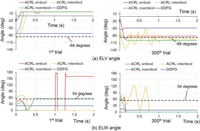
Figure 7a shows the comparisons of time histories of the ELV angle at
the 1st trial and 300th trial between the four cases. The vertical axis ranges
Downloaded from http://www.mitpressjournals.org/doi/pdf/10.1162/neco_a_01333 by guest on 16 March 2021148 M. Iwamoto and D. Kato
Figure 7: Comparisons of time histories of ELV and ELW angles among the four
models: ACRL embod, ACRL mlembod, ACRL noembod, and DDPG. (a) ELV
angle. (b) ELW angle. ELV, elbow flexion-extension; ELW, elbow inversion-
eversion.
of ELV in Figure 7a and ELW, SHU, SHV, and SHW in Figures 7b, 8, and
9 correspond to the angle rangles of ELV, ELW, SHU, SHV, and SHW de-
fined in section 2.2, respectively. ACRL embod and ACRL mlembod held
the joint angle of elbow flexion-extension on the target angle of −88 de-
grees at the 300th trial. ACRL noembod was close to the target angle at the
300th trial, but DDPG did not achieve it. Figure 7b shows the comparisons
of time histories of the ELW angle at the 1st and 300th trials between the
four cases. ACRL noembod held the joint angle of elbow inversion-eversion
on the target angle of 54 degrees at the 1st trial, but it did not achieve the
target angle at the 300th trial. ACRL embod and ACRL mlembod tended
to achieve the target in the initial period from 0 to 0.2 s at the 300th trial.
However, the other cases did not achieve the target angle. Figure 8a shows
the comparisons of time histories of the SHU angle at the 1st and 300th tri-
als between the four cases. ACRL mlembod held the joint angle of shoulder
internal-external rotation on the target angle of −39 degrees at the 300th
trial. The other cases did not achieve the target angle. Figure 8b shows the
comparisons of time histories of the SHV angle at the 1st and 300th trials
between the four cases. ACRL mlembod held the joint angle of shoulder
flexion-extension on the target angle of −36 degrees at the 300th trial. The
other cases did not achieve the target angle. Figure 9 shows the compar-
isons of time histories of the SHW angle at the 1st and 300th trials between
Downloaded from http://www.mitpressjournals.org/doi/pdf/10.1162/neco_a_01333 by guest on 16 March 2021ACRL With Embodiment for Arm Stabilization 149
Figure 8: Comparisons of time histories of SHU and SHV angles among the four
models: ACRL embod, ACRL mlembod, ACRL noembod, and DDPG. (a) SHU
angle. (b) SHV angle. SHU, shoulder internal-external rotation; SHV, shoulder
flexion-extension.
Figure 9: Comparisons of time histories of SHW angle among the four mod-
els: ACRL embod, ACRL mlembod, ACRL noembod, and DDPG. (a) First trial.
(b) Three-hundredth trial. SHW, shoulder inversion-eversion.
the four cases. ACRL mlembod held the joint angle of shoulder inversion-
eversion on the target angle of 36 degrees at the 300th trial. The other cases
did not achieve the target angle.
Figure 10 shows time-history curves of the muscle activation levels of
flexors and extensors of the elbow joint and flexors and extensors and ad-
ductors and abductors of the shoulder joint at the 300th trial in ACRL em-
bod and ACRL mlembod, which tended to realize posture stabilization at
target angles. The biceps brachii long head, brachialis, and brachioradialis
are the flexors of the elbow joint, while the triceps brachii long head is an
Downloaded from http://www.mitpressjournals.org/doi/pdf/10.1162/neco_a_01333 by guest on 16 March 2021150 M. Iwamoto and D. Kato
Figure 10: Time histories of muscle activation levels of flexors and extensors of
the elbow joint and flexors and extensors and adductors and abductors of the
shoulder joint at the 300th trial in ACRL embod and ACRL mlembod. (a) ACRL
embod. (b) ACRL mlembod. The biceps brachii long head, brachialis, and bra-
chioradialis are flexors of the elbow joint, while the triceps brachii long head is
an extensor of the elbow joint. The deltoid anterior, coracobrachialis, and biceps-
brachii long head are flexors of the shoulder joint, while the deltoid posterior
is an extensor of the shoulder joint. The teres major and subscapularis are ad-
ductors of the shoulder joint, while the deltoid middle and supraspinatus are
abductors of the shoulder joint. ACRL embod, ACRL with an embodiment us-
ing equations 2.21 to 2.40; ACRL mlembod, ACRL with an embodiment using
equation 2.41.
extensor of the elbow joint. The deltoid anterior, coracobrachialis, and bi-
ceps brachii long head are flexors of the shoulder joint, while the deltoid
posterior is an extensor of the shoulder joint. The teres major and sub-
scapularis are adductors of the shoulder joint, while the deltoid middle and
supraspinatus are abductors of the shoulder joint. Figure 7a shows that in
ACRL embod, the initial angle of ELV was −20 degrees, and ACRL embod
held the angle at −82 degrees, close to the target angle of −88 degrees, at
the 300th trial. Activation levels of the brachialis and brachioradialis ini-
tially increased to flex the elbow joint to the target angle. However, because
the elbow joint angle exceeded the target angle, the triceps brachii long head
muscle increased to extend the elbow joint, and the flexors and extensors
were then mutually antagonized to hold the posture (see Figure 10a). In
ACRL mlembod, the initial angle of ELV was −61 degrees, and the angle
then approached the target angle with some fluctuations around the target
angle at the 300th trial. The flexors and extensors of the elbow joint were
mutually antagonized to hold the posture (see Figure 10b). Figure 8a shows
Downloaded from http://www.mitpressjournals.org/doi/pdf/10.1162/neco_a_01333 by guest on 16 March 2021ACRL With Embodiment for Arm Stabilization 151
that in ACRL mlembod, the initial angle of SHU was −24 degrees, and the
angle then tended to hold the posture with some fluctuation around the tar-
get angle at the 300th trial. Activation levels of adductors and abductors of
the shoulder joint were mutually antagonized to hold the posture (see Fig-
ure 10b). In ACRL embod, the initial angle of SHU was −43 degrees, and the
adductors of the shoulder joint were activated to achieve the target angle of
−39 degrees; however, the shoulder joint angle had extensive internal rota-
tions to 10 degrees, and the abductors could not return to the target angle at
the 300th trial. Figure 8b shows that in ACRL mlembod, the initial angle of
SHV was −64 degrees, and the angle then approached the target angle of
−36 degrees with some fluctuations around the target angle at the 300th
trial. Activation levels of flexors and extensors of the shoulder joint were
mutually antagonized to hold the posture (see Figure 10b). In ACRL em-
bod, the initial angle of SHV was 5 degrees, and the flexors of the shoulder
joint were activated to achieve the target angle of −36 degrees; however, the
shoulder joint angle had extensive flexion to −67 degrees, and the extensors
could not return to the target angle at the 300th trial.
4 Discussion
In this study, we developed a novel muscle controller in which the ACRL
method can produce the muscle activation level of each muscle in a mus-
culoskeletal model of the right upper extremity of a human adult male and
acquire better activation control policy for posture stabilization of the five
joint motions of the human arm under gravity. Previous studies (Min et al.,
2018; Kambara et al., 2004) have successfully obtained activation control
policy for posture stabilization of the elbow joint or both the elbow and
shoulder joints under gravity. The control policy obtained by the ACRL
model of Min et al. (2018) demonstrated posture stabilization of the flexion-
extension of the elbow joint even when a weight was loaded on the hand.
However, the computational costs for learning were too high, and 700 trials
were needed. The control policy obtained by the ACRL model of Kambara
et al. (2004) also demonstrated posture stabilization of the flexion-extension
motions of the elbow and shoulder joints; however, the computational costs
for learning were too high: 22,500 trials were needed.
There are some limitations regarding the lower computational efficiency
of the application of RL to real-world problems, including robot controls.
That is, sufficient learning is not achieved with an insufficient number of
trials, and the value of reward function does not increase. Thus, some coun-
termeasures have been proposed by some researchers (Silver et al., 2014;
Popov et al., 2018; Andrychowicz et al., 2017). As mentioned in section
1, their methodology to realize efficient learning is focused on the inter-
nal control system with RL, which corresponds to the brain. In this study,
we focused on embodiment that can efficiently control walking or balanc-
ing in dynamic environments, as Hoffmann and Pfeifer (2012) suggested,
Downloaded from http://www.mitpressjournals.org/doi/pdf/10.1162/neco_a_01333 by guest on 16 March 2021152 M. Iwamoto and D. Kato
and introduced two types of AFMs that control muscle tone for mutually
antagonizing muscles such as flexors and extensors, adductors and abduc-
tors, and invertors and evertors into the output of the actor in the actor-
critic method as information on the embodiment of a human being. The first
AFM, which corresponds to ACRL embod, is described based on the differ-
ences in the five joint motions, while the second AFM, which corresponds
to ACRL mlembod, is described based on the length rate of each muscle.
We compared simulation results between the learning methods with AFMs
and those without AFMs. We found that in ACRL embod, the reward grad-
ually increased to 8.6, and the value was maintained until the 300th trial;
furthermore, the posture of flexion-extension (ELV) of the elbow joint was
stabilized at their corresponding target angles at the 300th trial. In ACRL
mlembod, the reward gradually increased to 8.5 but decreased to 8.2 at the
300th trial. However, the postures of the five joint motions were almost sta-
bilized at the corresponding target angles at the 300th trial, although the
postures had some fluctuations around the target angles. In contrast, in the
learning methods without any AFMs, ACRL noembod, and DDPG, the pos-
tures of the five joint motions were not stabilized at the target angles at the
300th trial. These simulation results suggest that the proposed method with
AFMs realized posture stabilization at the predetermined target angles of
the five joint motions of the human arm at a relatively earlier period of learn-
ing. These results suggest that the introduction of AFMs as embodiment of
muscle tone can stabilize the posture of human musculoskeletal models and
stabilize the joint motions of a humanoid robot, including muscular struc-
ture under gravity, with efficient learning costs.
The AFMs proposed in this study represent functions of the PPTn and
MLR for mutually antagonizing muscles such as flexors and extensors, ad-
ductors and abductors, and invertors and evertors, and modulate the max-
imum values of the activation levels of the mutually antagonizing muscles,
in which the activation levels are signals from the SNr, that is, an actor of
ACRL. In our proposed models, we hypothesized that changes in each joint
angle from each neutral angle, which was determined as space attitude in
this study, can control the activation levels of each muscle. For example,
in the case of elbow flexion-extension, the change in the flexed elbow joint
angle from the neutral angle can increase the activation levels of extensors
and decrease those of the flexors, whereas the change in the extended joint
angle from the neutral angle can increase the activation levels of flexors and
decrease those of extensors in posture stabilization; the same holds in the
other joint motions.
We implemented the feature in two types of AFMs corresponding to
ACRL embod and ACRL mlembod. In ACRL embod, the postures were sta-
bilized for ELV; however, the postures were not stabilized for ELW, SHU,
SHV, and SHW. The reason SHU and SHV were not stabilized on the tar-
get angles are probably because the musculoskeletal model did not include
sufficient abductors and extensors of the shoulder joint to control SHU and
Downloaded from http://www.mitpressjournals.org/doi/pdf/10.1162/neco_a_01333 by guest on 16 March 2021You can also read