Learning Bijective Feature Maps for Linear ICA
←
→
Page content transcription
If your browser does not render page correctly, please read the page content below
Learning Bijective Feature Maps for Linear ICA

                        Alexander Camuto*,1,3                  Matthew Willetts*,1,3
                  Brooks Paige   2,3
                                          Chris Holmes     1,3
                                                                     Stephen Roberts1,3
                1
                  University of Oxford 2
                                         University College London    3
                                                                        Alan Turing Institute

                      Abstract                                In particular, flow-based models have been proposed as
                                                              a non-linear approach to square ICA, where we assume
     Separating high-dimensional data like images             the dimensionality of our latent source space is the same
     into independent latent factors, i.e indepen-            as that of our data (Deco & Brauer, 1995; Dinh et al.,
     dent component analysis (ICA), remains an                2015). Flows parameterise a bijective mapping between
     open research problem. As we show, existing              data and a feature space of the same dimension and can
     probabilistic deep generative models (DGMs),             be trained via maximum likelihood for a chosen base
     which are tailor-made for image data, under-             distribution in that space. While these are powerful
     perform on non-linear ICA tasks. To address              generative models, for image data one typically wants
     this, we propose a DGM which combines bijec-             fewer latent variables than the number of pixels in an
     tive feature maps with a linear ICA model to             image. In such situations, we wish to learn a non-square
     learn interpretable latent structures for high-          (dimensionality-reducing) ICA representation.
     dimensional data. Given the complexities of
     jointly training such a hybrid model, we in-             In this work, we highlight the fact that existing proba-
     troduce novel theory that constrains linear              bilistic deep generative models (DGMs), in particular
     ICA to lie close to the manifold of orthogo-             Variational Autoencoders (VAEs), underperform on
     nal rectangular matrices, the Stiefel manifold.          non-linear ICA tasks. As such there is a real need
     By doing so we create models that converge               for a probabilistic DGM that can perform these tasks.
     quickly, are easy to train, and achieve better           To address this we propose a novel methodology for
     unsupervised latent factor discovery than flow-          performing non-square non-linear ICA using a model,
     based models, linear ICA, and Variational                termed Bijecta, with two jointly trained parts: a highly-
     Autoencoders on images.                                  constrained non-square linear ICA model, operating on
                                                              a feature space output by a bijective flow. The bijective
1    Introduction                                             flow is tasked with learning a representation for which
                                                              linear ICA is a good model. It is as if we are learning
In linear Independent Component Analysis (ICA), data
                                                              the data for our ICA model.
is modelled as having been created from a linear mixing
of independent latent sources (Cardoso, 1989a,b, 1997;        We find that such a model fails to converge when trained
Comon, 1994). The canonical problem is blind source           naively with no constraints. To ensure convergence,
separation; the aim is to estimate the original sources of    we introduce novel theory for the parameterisation of
a mixed set of signals by learning an unmixing matrix,        decorrelating, non-square ICA matrices that lie close
which when multiplied with data recovers the values of        to the Stiefel manifold (Stiefel, 1935), the space of or-
these sources. While linear ICA is a powerful approach        thonormal rectangular matrices. We use this result to
to unmix signals like sound (Everson & Roberts, 2001),        introduce a novel non-square linear ICA model that
it has not been as effectively developed for learning          uses Johnson-Lidenstrauss projections (a family of ran-
compact representations of high-dimensional data like         domly generated matrices). Using these projections,
images, where assuming linearity is limiting. Non-            Bijecta successfully induces dimensionality reduction
linear ICA methods, which assume non-linear mixing            in flow-based models and scales non-square non-linear
of latents, offer better performance on such data.             ICA methods to high-dimensional image data. Further
                                                              we show that it is better able to learn independent la-
*Equal Contribution.
                                                              tent factors than each of its constituent components in
Proceedings of the 24th International Conference on Artifi-
cial Intelligence and Statistics (AISTATS) 2021, San Diego,   isolation and than VAEs. For a preliminary demonstra-
California, USA. PMLR: Volume 130. Copyright 2021 by          tion of the inability of VAEs and the ability of Bijecta
the author(s).                                                to discover ICA sources see Fig 1.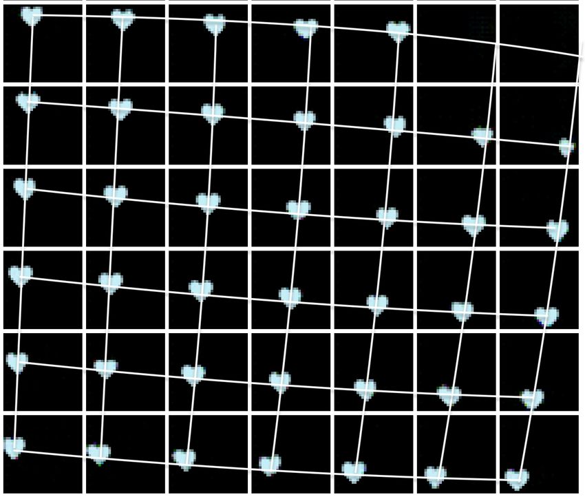
Learning Bijective Feature Maps for Linear ICA
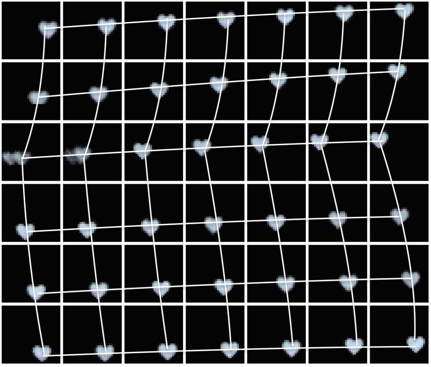
(a) Sample Images
(b) VAE Sources (c) Bijecta Sources
Figure 1: Here we take a dSprites heart and, using a randomly sampled affine transformation, move it around a
black background (a). The underlying sources of the dataset are affine transformations of the heart. In (b-c)
images in the center correspond to the origin of the learnt source space. Images on either side correspond to
linearly increasing values along one of the learnt latent sources whilst the other source remains fixed. Bijecta (c)
has learned affine transformations as sources (white diagonals), whereas a VAE (with ICA-appropriate prior) (b)
has learned non linear transforms (white curves). The VAE has not discovered the underlying latent sources.
2 Background priors as it allows for the specification of a sub or super
Gaussian distribution by way of a single parameter: ⇢.
2.1 Independent Component Analysis
The goal of ICA is to learn a set of statistically in- 2.2 Manifolds for the unmixing matrix A+
dependent sources that ‘explain’ our data. ICA is a In linear ICA we want to find the linear mapping A+
highly diverse modelling paradigm with numerous vari- resulting in maximally independent sources. This is
ants: learning a mapping vs learning a model, linear more onerous than merely finding decorrelated sources,
vs non-linear, different loss functions, different genera- as found by principal component analysis (PCA).
tive models, and a wide array of methods of inference
When learning a linear ICA model we typically have
(Cardoso, 1989a; Mackay, 1996; Lee et al., 2000).
the mixing matrix A as the (pseudo)inverse of the
Here, we specify a generative model and find point-wise unmixing matrix A+ and focus on the properties of
maximum likelihood estimates of model parameters in A+ to improve convergence. A+ linearly maps from
the manner of (Mackay, 1996; Cardoso, 1997). Con- the data-space X to the source space S. It can be
cretely, we have a model with latent sources s 2 S = decomposed into two linear operations. First we whiten
Rds generating data x 2 X = Rdx , with ds dx . The the data such that each component has unit variance
linear ICA generative model factorises as and these components are mutually uncorrelated. We
ds
Y then apply an orthogonal transformation and a scaling
p(x, s) = p(x|s)p(s), p(s) = p(si ), operation (Hyvärinen et al., 2001, §6.34) to ‘rotate’
i=1 the whitened data into a set of coordinates where the
where p(s) is a set of independent distributions appro- sources are independent and decorrelated. Whitening
priate for ICA. In linear ICA, where all mappings are on its own is not sufficient for ICA — two sources can
simple matrix multiplications, the sources cannot be be uncorrelated and dependent (see Appendix A).
Gaussian distributions. Recall that we are mixing our
sources to generate our data: A linear mixing of Gaus- Thus we can write the linear ICA unixing matrix as
sian random variables is itself Gaussian, so unmixing A+ = RW (2)
is impossible (Lawrence & Bishop, 2000). To be able
where W 2 Rds ⇥dx is our whitening matrix, R 2
to unmix, to break this symmetry, we can choose any
Rds ⇥ds is an orthogonal matrix and 2 Rds is a
heavy-tailed or light-tailed non-Gaussian distribution
diagonal matrix. Matrices that factorise this way
as our prior p(s) that gives us axis alignment and in-
are known as the decorrelating matrices (Everson &
dependence between sources. A common choice is the
Roberts, 1999): members of this family decorrelate
family of generalised Gaussian distributions,
through W, and R ensures that sources are statisti-
p(si ) = GG(si |µ, ↵, ⇢) cally independent, not merely uncorrelated. The opti-
✓ ◆⇢ mal ICA unmixing matrix is the decorrelating matrix
⇢ |si µ|
p(si ) = exp (1) that decorrelates and gives independence.
2↵ (1/⇢) ↵
with mean µ, scale ↵ and shape ⇢. For ⇢ = 2 we recover 2.3 Flows
the Normal distribution, and for ⇢ = 1 we have the Flows are models that stack numerous invertible
(heavy-tailed) Laplace. As ⇢ ! 1 the distribution changes of variables. One specifies a simple base distri-
becomes increasingly sub-Gaussian, tending to a uni- bution and learns a sequence of (invertible) transforms
form distribution. As such, the generalised Gaussian to construct new distributions that assign high proba-
is a flexible framework for specifying ICA-appropriate bility to observed data. Given a variable z 2 Z = Rdx ,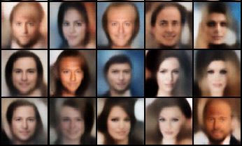
Alexander Camuto*, Matthew Willetts*, Brooks Paige, Chris Holmes Stephen Roberts

we specify the distribution over data x as                   soft supervision, is key to getting appropriate repre-
                                          1                  sentations (Rolinek et al., 2019; Locatello et al., 2019).
                                    @f
                p(x) = p(z) det               ,      (3)     Stühmer et al. (2019) obtains a variety of non-linear
                                     @z
                                                             ICA using VAEs with sets of Generalised Gaussian pri-
where f is a bijection from Z ! X , ie Rdx ! Rdx , and       ors, but even then penalisation is required to obtain
p(z) is the base distribution over the latent z (Rezende    ’disentangled’ representations.
& Mohamed, 2015; Papamakarios et al., 2019).                As such there is a need for probabilistic DGMs that can
For more flexible distributions for x, we specify x         separate sources without added hyperparameter tuning
through a series of composed functions, from our sim-       and that can do so by matching ICA-appropriate priors.
ple initial p into a more complex multi-modal distri-       Our solution combines linear ICA with a dimensionality-
bution; for example for a series of K + 1 mappings,         preserving invertible flow f✓ . The flow acts between our
z = fK ... f0 (x). By the properties of determinants        data space of dimensionality and the representation
under function composition                                  fed to the linear ICA generative model; learning a
                             K
                                                            representation that is well fit by the simple, linear ICA
                             Y           @fi 1              model. As we demonstrate in experiments (§5), this
             p(x) = p(zK )         det         ,     (4)
                             i=0
                                         @zi+1              hybrid model, which we call Bijecta, succeeds where
                                                            VAEs fail: it can match non-Gaussian priors and is
where zi+1 denotes the variable resulting from the          able to discover independent latent sources on image
transformation fi (zi ), p(zK ) defines a density on the    datasets.
K th , and the bottom most variable is our data (z0 = x).
                                                      1     3.1   A Linear ICA base distribution for flows
Computing the determinant of the Jacobian (det @f@z )
                                                            Our aim here is to develop a non-square ICA method
in Eq. (3) can be prohibitively costly, especially when
                                                            that is both end-to-end differentiable and computation-
composing multiple functions as in Eq. (4). To address
                                                            ally efficient, such that it can be trained jointly with
this, flows use coupling layers that enforce a lower
                                                            a flow via stochastic gradient descent. We begin by
triangular Jacobian such that the determinant of the
                                                            choosing our base ICA source distribution to be a set of
Jacobian is simply the product of its diagonal elements.
                                                            independent generalised Gaussian distributions, Eq (1)
We use recently proposed coupling layers based on ra-
                                                            with µ = 0, ↵ = 1 and ⇢ varying per experiment; and
tional quadratic splines (RQS) to enforce this lower
                                                            the ICA model’s likelihood to a be a Gaussian.
triangular structure (Durkan et al., 2019). They form
highly flexible flows that typically require fewer com-       p(si ) = GG(si |µ = 0, ↵ = 1, ⇢), for i 2 {1, . . . , ds },
posed mappings to achieve good performance relative           p(z|s) = N (x|As, ⌃✓ ),
to other coupling layers. See Appendix H for details.
                                                            where A 2 Rdx ⇥ds is our (unknown) ICA mixing ma-
3   Non-Square ICA using Flows                              trix, which acts on the sources to produce a linear mix-
                                                            ture; and ⌃✓ is a learnt or fixed diagonal covariance.
Variational Autoencoders seem like a natural fit for
                                                            This linear mixing of sources yields an intermediate
learning a compressed set of statistically independent
                                                            representation z that is then mapped to the data by
latent variables (Kingma & Welling, 2014; Rezende
                                                            a flow. Our model has three sets of variables: the
et al., 2014). It seems natural to train a VAE with
                                                            observed data x, the flow representation z = f 1 (x),
an appropriate non-Gaussian prior, and expect that
                                                            and ICA latent sources s. It can be factorised as
it would learn an appropriate ICA model. However,
this is not the case. In Khemakhem et al. (2020) some                                                        @f✓ 1
                                                               p✓ (x, s) = p✓ (x|s)p(s) = p(z|s)p(s) det                (5)
experiments suggest that VAEs with ICA-appropriate                                                            @z
priors are unsuited to performing non-linear ICA. In our
experiments (§5) we further verify this line of inquiry     While it is simple to train a flow by maximum likelihood
and show that VAEs struggle to match their aggregate        method when we have a simple base distribution in
posteriors to non-Gaussian priors and thus are unable       Z, here to obtain a maximum likelihood objective we
to discover independent latent sources.                     would have to marginalise out s to obtain the evidence
                                                            in Z; a computationally intractable procedure:
Though source separation can be achieved by ‘disen-                                  Z
tangling’ methods such as the -VAE (Higgins et al.,                 p(z; A, ⌃✓ ) = ds p(z|s; A, , ⌃✓ )p(s).       (6)
2017) and -TCVAE (Chen et al., 2018), these meth-
ods require post-hoc penalisation of certain terms of       A contemporary approach is to use amortised varia-
the VAE objective, at times inducing improper priors        tional inference for the linear ICA part of our model.
(in the -TCVAE in particular (Mathieu et al., 2019)).       This means we introduce an approximate amortised
Further, precise tuning of this penalisation, a form of     posterior for s and perform importance sampling on
Learning Bijective Feature Maps for Linear ICA
ing a linear model with a powerful flow was not trivial
A ⌃✓ ✓ A+ b ✓ and models failed to converge when naively optimising
Eq (8). We found it crucial to appropriately constrain
s z x s z x the unmixing matrix to get models to converge. We
detail these constraints in the next section.
N N
(a) Generative Model (b) Variational Posterior 4 Whitening in A+ , without SVD
Figure 2: The generative model (a) and variational What are good choices for the mixing and unmixing
posterior (b), as defined in Eq (8). matrices? Recall in Sec 2.2 we discussed various tradi-
tional approaches to constraining the unmixing matrix.
For our flow-based model, design choices as to the pa-
Eq (6), taking gradients through our samples using rameterisation of A+ stabilise and accelerate training.
the reparameterisation trick (Kingma & Welling, 2014; As before, the mixing matrix A is unconstrained during
Rezende et al., 2014). Amortised stochastic variational optimisation. However, without the constraints on A+
inference offers numerous benefits: it scales training to we describe in this section, we found that joint training
large datasets by using stochastic gradient descent, our of a flow with linear ICA did not converge.
trained model can be applied to new data with a simple
forward pass, and we are free to choose the functional Recall Eq (2) — linear ICA methods carry out whiten-
& probabilistic form of our approximate posterior. Fur- ing W, performing dimensionality reduction projecting
ther our ICA model is end-to-end differentiable, making from a dx -dimensional space to a ds -dimensional space,
it optimal for jointly training with a flow. and the remaining rotation and scaling operations are
square. When training with a flow the powerful splines
We choose a linear mapping in our posterior, with we are learning can fulfill the role of the square matrices
q (s|z) = Laplace(s|A+ z, b ), where we have intro- R and , but doing this ahead of the whitening itself.
duced variational parameters = {A+ , b } corre- Put another way, the outputs from the flow can be
sponding to an unmixing matrix and a diagonal diver- learnt such that they are simply a whitening operation
sity. Using samples from this posterior we can define a away from being effective ICA representations in S.
lower bound L on the evidence in Z Thus, to minimise the complexities of jointly training a
log p(z; A,⌃✓ ) L(z; , A, ⌃✓ ) powerful flow with a small linear model, we can simply
= Es⇠q [log p(z|s) KL(q (s|z)||p(s)) (7) set A+ = W, such that the unmixing matrix projects
Using the change of variables equation, Eq (3), and the from dz to ds and is decorrelating. Statistical indepen-
lower bound on the evidence for ICA in (7) for Z, we dence will come from the presence of the KL term in
can obtain a variational lower bound on the evidence Eq (7): the flow will learn to give z representations
for our data x as the sum of the ICA model’s ELBO that, when whitened, are good ICA representations in
(acting on z) and the log determinant of the flow: S. See Fig 3 for a visual illustration of this process and
a comparison with the steps involved in linear ICA.
log p✓ (x; A,⌃✓ ) L(x; ✓, , A, ⌃✓ )
@f✓ 1 In previous linear ICA methods, the whitening pro-
= L(z; , A, ⌃✓ ) + log det (8) cedure W has been derived in some data-aware way.
@z
A common choice is to whiten via the Singular Value
As such our model is akin to a flow model, but with
Decomposition (SVD) of the data matrix, where W =
an additional latent variable s; the base distribution
⌃UT , ⌃ is the rectangular diagonal matrix of singular
p(z) of the flow is defined through marginalizing out
values of X, and the columns of U are the left-singular
the linear mixing of the sources. We refer to a model
vectors. Computing the SVD of the whole dataset is
with n non-linear splines mapping from X to Z as an
expensive for large datasets; for us, in the context of
n-layer Bijecta model.
Bijecta, we would be re-calculating the SVD of the
In the case of non-square ICA, where our ICA model representations Z = f 1 (X) of the entire dataset after
is not perfectly invertible, errors when reconstructing every training step. One route around this would be
a mapping from S to Z may amplify when mapping online calculation of the whitening matrix (Cardoso &
back to X . To mitigate this we add an additional reg- Laheld, 1996; Hyvärinen et al., 2001). This introduces
ularisation term in our loss that penalises the L1 error an extra optimisation process that also has to be tuned,
of each point when reconstructed into X . This penali- and would interact with the training of the flow.
sation can be weighted according to the importance of
To tackle these shortcomings of existing whitening
high-fidelity reconstructions for a given application.
methods, we propose a new method for linear non-
We attempted to train Bijecta with unconstrained mix- square ICA that uses Johnson–Lindenstrauss (JL)
ing and unmixing matrices, but found that jointly train- transforms (also known as sketching) (Woodruff, 2014),Alexander Camuto*, Matthew Willetts*, Brooks Paige, Chris Holmes Stephen Roberts
(a) Linear ICA (b) Bijecta
Figure 3: (a) Sequence of actions that are performed by the elements of A+ , the unmixing matrix of linear ICA.
W whitens the correlated data and R then ensures that the whitened (decorrelated) data is also independent.
(b) Sequence of actions that are performed by the elements of Bijecta. f 1 maps data to a representation for which
the whitening matrix is the ICA matrix. W now whitens f 1 (x) and the result is also statistically independent.
which not only works effectively as a linear ICA method, the Stiefel manifold V(r, c) the off-diagonal elements of
but also works in conjunction with a flow model. These the cross-correlation matrix of the projection GX are
JL transforms have favourable properties for ICA, as ever smaller, so G is ever more decorrelating. Given
we demonstrate in theoretical results. Further, this these properties we want our whitening matrix to lie
method samples part of the whitening matrix at initial- close to the Stiefel manifold.
isation and leaves it fixed for the remainder of training,
requiring no hyper-parameter tuning and making it 4.1.1 Johnson-Lindenstrauss projections
extremely computationally efficient. This method is By Theorem 1 we know that we want our whitening
novel and efficient when used as a whitening method matrix to be close to V(ds , dx ). How might we enforce
within linear ICA, and when combined with a flow as this closeness? By the definition of the Stiefel manifold,
in Bijecta is a powerful method for non-linear ICA as we can intuit that a matrix G will lie close to this
we demonstrate in experiments. manifold if GGT ⇡ I. We formalise this as:
4.1 Approximately-Stiefel matrices Theorem 2. Let G 2 Rds ⇥dx and let G̃ be its
We have set A+ = W, the whitening matrix. W has projection onto V(ds , dx ). As the Frobenius norm
two aims in non-square ICA. The first is dimensional- kGGT Ik ! 0, we also have kG̃ Gk ! 0.
ity reduction, projecting from a dx -dimensional space The proof for this is presented in Appendix D. Us-
to a ds -dimensional space. The second is to decorre- ing this theorem, we now propose an alternative to
late the data it transforms, meaning that the resulting SVD-based whitening. Instead of having W = ⌃ 1 UT
projection will have unit variance and mutually uncor- be the result of SVD on the data matrix, we define
related components. More formally we wish for W of our whitening matrix as a data-independent John-
dimensionality ds ⇥ dx to be decorrelating. son–Lindenstrauss transform. We must ensure that W,
The set of orthogonal decorrelating rectangular matri- our rectangular matrix, is approximately orthogonal,
ces lie on the Stiefel Manifold (Stiefel, 1935) denoted lying close to the manifold V(ds , dx ). More formally
V. For matrices with r rows and c columns, a matrix by Theorem 2, our goal is to construct a rectangular
G 2 V(r, c) iff GG⇤ = I (G⇤ the conjugate transpose matrix W such that WWT ⇡ I.
of G). Constraining the optimisation of W to this man- We construct approximately orthogonal matrices for
ifold can be computationally expensive and complex W by way of Johnson-Lindenstrauss (JL) Projections
(Bakir et al., 2004; Harandi & Fernando, 2016; Siegel, (Johnson & Lindenstrauss, 1984). A JL projection W
2019) and instead we choose for W to be approximately for Rdx ! Rds is sampled at initialisation from a simple
Stiefel, that is to lie close to V(ds , dx ). This is justified binary distribution Achlioptas (2003):
by the following theorem, proved in Appendix A: ( p
+1/ ds , with probability 12
Theorem 1. Let G be a rectangular matrix and G̃ be Wi,j = p (9)
its projection onto V(r, c). As the Frobenius norm ||G 1/ ds , with probability 12
G̃|| ! 0 we have that ||GXXT GT || ! 0, where
This distribution satisfies E[WWT ] = I, and such
GXXT GT is the cross-correlation of the projection of
a draw has WWT ⇡ I. We choose to fix W after
data X by G, and is some diagonal matrix.
initialisation such that A+ = W never updates, greatly
Simply put, this shows that as a matrix G approaches simplifying optimisation.Learning Bijective Feature Maps for Linear ICA
(a) Source Images (b) Mixed (c) A FastICA (d) A JL-Cayley ICA
Figure 4: Here we run linear ICA on a pair of images (a) that are mixed linearly (mix = w1 ⇤ image1 + w2 ⇤ image2 )
(b) to form a dataset with 512 points. In both cases w1 and w2 are sampled from a uniform distribution. We plot
the mixing matrix A for our JL-Cayley model with a quasi-uniform GG prior with ⇢ = 10 (c) and for FastICA
(Hyvärinen & Oja, 1997) as a benchmark. A should recover the source images, which occurs for both models.
(a) Sample Images
(b) VAE Latent Traversals (c) Bijecta Latent Traversals
Figure 5: Here we demonstrate that Bijecta is capable of unmixing non-linearly mixed sources, better than VAEs
with ICA-appropriate priors. We take a dSprites heart and, using a randomly sampled affine transformation,
move it around a 32 by 32 background (a). With 2-D GG priors with ⇢ = 10 for a convolutional VAE (b) and for
Bijecta (c) we plot the generations resulting from traversing the 2-D latent-source space in a square around the
origin. We sketch the learnt axis of movement of the sprite with white lines. In (b) the VAE does not ascribe
consistent meaning to its latent dimensions. It has failed to discover consistent independent latent sources: it
has a sudden change in the learnt axes of movement along the second dimension, as seen by the kink in the
white vertical lines. In (c) Bijecta is able to learn a simple affine transformation along each latent dimension,
consistently spanning the space. In Fig B.2 we show the posterior distributions of both these models and show
that Bijecta is better able to match the GG prior than the VAE, supporting our findings here.
5 Experiments heart. First, in Fig B.2 we demonstrate that linear ICA
models are unable to uncover the true latent sources.
Here we show that our approach outperforms VAEs As expected non-linear mixing regimes motivate the
and flows with ICA-priors at discovering ICA sources use of flexible non-linear models.
in image data. But first, as a sanity check, we show
that a linear ICA model using JL projections to whiten We now demonstrate that Bijecta can uncover the la-
can successfully unmix linearly mixed sources in Fig tent sources underpinning these affine transformations,
4. For details on how to implement such a linear ICA whereas VAEs with ICA-appropriate priors fail to do
model, see Appendix E. We take a pair of images from so. For details of VAE architecture, see Appendix I.
dSprites and create linear mixtures of them. We see These VAEs are able to learn to reconstruct data well,
that linear ICA with JL projections can successfully but the learnt latent space does not correspond to the
discover the true sources, the images used to create the underlying statistically independent sources (see Figs
mixtures, in the columns of A. 1 and B.2). In fact for VAEs the effect of the latent
variables is not consistent throughout the latent space,
Affine Data Given that we have established that as seen in Fig 5. For Bijecta, the learnt latent space
our novel theory for decorrelating matrices can pro- corresponds to the underlying statistically independent
duce standalone linear ICA models, we now want to sources (see Figs 1 and B.2), and the meaning of the
ascertain that our hybrid model performs well in non- latent variables is consistent in Fig 5. Further in Fig 5
linear mixing situations. To do so we create a dataset the model seems able to extrapolate outside the train-
consisting of a subset of dSprites where we have a light- ing domain: it generates images where the heart is
blue heart randomly uniformly placed on a black field. partially rendered at the edges of the frame, even re-
The true latent sources behind these randomly sampled moving the heart entirely at times, even though such
affine transformations are simply the coordinates of the images are not in the training set.Alexander Camuto*, Matthew Willetts*, Brooks Paige, Chris Holmes Stephen Roberts
(a) Bijecta Factorised Posterior (b) Bijecta latent 5 traversal (c) RQS flow traversal
Figure 6: (a) shows decodings from an 8-layer Bijecta (ds = 32) trained on CelebA with a Laplace prior (GG
⇢ = 1) where we sample from the factorised approximation to Bijecta’s posterior. See Fig J.6 for more such
samples. (b) shows latent traversals for 3 different datapoints all along the same axis-aligned direction, for this
same model. (c) shows traversals for a single embedded training datapoint from CelebA moving along 3 latent
directions in an RQS flow with Laplace base distribution. Though we have selected 3 dimensions, all Z dimensions
had similar latent traversals. In (b-c) Images in the center correspond to the original latent space embedding, on
either side we move up to 6 standard deviations away along this direction with other dimensions remaining fixed.
The flow has not discovered axis-aligned transforms, whereas Bijecta has learned informative latent dimensions:
here the dimension encodes hair thickness. Note that identity is maintained throughout and that the transform is
consistent across different posterior samples. See Appendix J.3 for gallery of transforms for Bijecta.
Natural Images The previous experiments show In Table 1, we show that Bijecta learns an aggregate
that our model is capable of isolating independent posterior with significantly lower TC values than both
sources on toy data. We complement this finding with VAEs with Laplace priors, and -TCVAEs – which in
experiments on a more complex natural image dataset, their training objective penalise the TC by a factor
CelebA, and show that here too our model outperforms (Chen et al., 2018). Our model has learnt a better
VAEs in learning factorisable representations. ICA solution. We also include numerical results in
Appendix J.1 showing that Bijecta outperforms linear
An ersatz test of this can be done by synthesising im- ICA on a variety of natural image datasets.
ages where we sample from a factorised approximation
of Bijecta’s posterior. If the learned latent sources are Table 1: Total Correlation Results: We evaluate the
actually independent, then the posterior over latent source separation of different models on CelebA via
sources given the entire dataset should factorize
Q into the TC of the validation set embeddings in the 32-
a product across dimensions, i.e. q(s) = i q(si ). In D latent space of: Laplace prior VAEs, -TCVAEs
this case, we can fit an approximation to the posterior ( = 15), and Bijecta with a Laplace prior (± indicates
by fitting ds independent one-dimensional density es- the standard deviation over 2 runs). VAEs use the
timates on q(si ). If the sources are not independent, same architecture and training as Chen et al. (2018).
then this factorized approximation to the posterior will
be missing important correlations and dependencies. Laplace-VAE -TCVAE Laplace-Bijecta
In Fig 6a samples from this factorised approximation
look reasonable, suggesting that Bijecta has learnt rep- TC: 106.7 ± 0.9 55.7 ± 0.1 13.1 ± 0.4
resentations that are statistically independent.
Dimensionality reduction on flow models To
To quantify this source-separation numerically, we mea-
conclude, having shown that Bijecta outperforms VAEs
sure the total correlation (TC) of the aggregate pos-
on a variety of non-linear ICA tasks, we now contrast
teriors of Bijecta (q(s|z)) and VAEs (q(z|x)) as Chen
our model’s ability to automatically uncover sources
et al. (2018) do. Intuitively, the TC measures how well
relative to flow models with heavy-tailed base distribu-
a distribution is approximated by the product of its
tions. We do so by measuring the cumulative explained
marginals – or how much information is shared between
variance by the dimensions in Z for both models. If
variables due to dependence (Watanabe, 1960). It di-
a small number of dimensions explains most of Z’s
rectly measures how well an ICA model has learnt decor-
variance then the model has learnt a bijection which
related and independent latent representations (Ever-
only requires a small number of dimensions to be in-
son & Roberts, 2001). Formally, it is the KL divergence
vertible. It has in effect learnt the generating sources
between a distribution r(·) and a factorisedQ represen-
underpinning the data.
tation of the distribution: TC = KL(r(s)|| i r(si )),
where i indexes over (latent) dimensions. In Fig 7 we show that Bijecta induces better-Learning Bijective Feature Maps for Linear ICA
Figure 7: Explained variance plots for the embedding in Z, as measured by the sums of the eigenvalues of the
covariance matrix of the embeddings, for both our Bijecta model and for an RQS model of equivalent size trained
with a Laplace base distribution (GG distribution with ⇢ = 1). For both Fashion-MNIST (left) and CIFAR 10
(right) datasets we see that the Bijecta model has learned a compressive flow, where most of the variance can be
explained by only a few linear projections. The shaded region denotes the first 64 dimensions, corresponding to
the size of the target source embedding S.
compressed representations in Z than non-compressive non-linear ICA models have been specified with addi-
flows. We plot the eigenvalues of the covariance matrix tional structure to reduce the space of potential solu-
on the output of the flow, i.e. on Cov(f (X)), to see tions, such as putting priors on variables (Lappalainen
how much of the total variance in the learned feature & Honkela, 2000) or specifying the precise non-linear
space Z can be explained in a few dimensions. In doing functions involved (Lee & Koehler, 1997; Taleb, 2002),
so we see that a flow trained jointly with a linear ICA Recent work shows that conditioning the source distri-
model with ds = 64 effectively concentrates variation butions on some always-observed side information, say
into a small number of intrinsic dimensions; this is in time index, can be sufficient to induce identifiability in
stark contrast with the RQS flows trained with only non-linear ICA (Khemakhem et al., 2020).
a Laplace base distribution. This demonstrates that
Modern flows were first proposed as an approach to
our model is able to automatically detect relevant di-
non-linear square ICA (Dinh et al., 2015), but are
rections on a low dimensional manifold in Z, and that
also motivated by desires for more expressive priors
the bijective component of our model is better able to
and posteriors (Kingma et al., 2016; Papamakarios
isolate latent sources than a standard flow.
et al., 2019). Early approaches, known as symplec-
For a visual illustration of this source separation we tic maps (Deco & Brauer, 1995; Parra et al., 1995,
show the difference in generated images resulting from 1996), were also proposed for use with ICA. Flows offer
smoothly varying along each dimension in S for Bijecta expressive dimensionality-preserving (and sometimes
models and in Z for flows in Fig 6. Bijecta is clearly volume-preserving) bijective mappings (Dinh et al.,
able to discover latent sources, whereby it learns axis- 2017; Kingma & Dhariwal, 2018). Flows have been
aligned transformations of CelebA faces, whereas a flow used to provide feature extraction for linear discrim-
with equivalent computational budget and a heavy- inative models (Nalisnick et al., 2019). Orthogonal
tailed base distribution is not able to. transforms have been used in normalizing flows before,
to improve the optimisation properties of Sylvester
All flow-based baselines are trained using the objective
flows (Van Den Berg et al., 2018; Golinski et al., 2019).
in Eq (4), using Real-NVP style factoring-out (Durkan
Researchers have also looked at constraining neural net-
et al., 2019; Dinh et al., 2015), and are matched in size
work weights to the Stiefel-manifold (Li et al., 2020).
and neural network architectures to the flows of Bijecta
models. See Appendix I for more details. 7 Conclusion
6 Related Work We have developed a method for performing non-linear
ICA large high-dimensional image datasets which com-
One approach to extend ICA to non-linear settings is
bines state-of-the-art flow-based models and a novel
to have a non-linear mapping acting on the indepen-
theoretically grounded linear ICA method. This model
dent sources and data (Burel, 1992; Deco & Brauer,
succeeds where existing probabilistic deep generative
1995; Yang et al., 1998; Valpola et al., 2003). In gen-
models fail: its constituent flow is able to learn a rep-
eral, non-linear ICA models have been shown to be
resentation, lying in a low dimensional manifold in
hard to train, having problems of unidentifiability: the
Z, under which sources are separable by linear un-
model has numerous local minima it can reach under
mixing. In source space S, this model learns a low
its training objective, each with potentially different
dimensional, explanatory set of statistically indepen-
learnt sources (Hyvärinen & Pajunen, 1999; Karhunen,
dent latent sources.
2001; Almeida, 2003; Hyvarinen et al., 2019). SomeAlexander Camuto*, Matthew Willetts*, Brooks Paige, Chris Holmes Stephen Roberts
Acknowledgments Cayley, A. (1846). Sur quelques propriétés des détermi-
This research was directly funded by the Alan Turing nants gauches. Journal für die reine und angewandte
Institute under Engineering and Physical Sciences Re- Mathematik, 32, 119–123.
search Council (EPSRC) grant EP/N510129/1. AC Chen, R. T. Q., Li, X., Grosse, R., & Duvenaud, D.
was supported by an EPSRC Studentship. MW was (2018). Isolating Sources of Disentanglement in Vari-
supported by EPSRC grant EP/G03706X/1. CH was ational Autoencoders. In NeurIPS.
supported by the Medical Research Council, the Engi-
Choudrey, R. (2000). Variational Methods for Bayesian
neering and Physical Sciences Research Council, Health
Independent Component Analysis. PhD thesis, Uni-
Data Research UK, and the Li Ka Shing Foundation
versity of Oxford.
SR gratefully acknowledges support from the UK Royal
Academy of Engineering and the Oxford-Man Institute. Comon, P. (1994). Independent component analysis, A
new concept? Signal Processing, 36(3), 287–314.
We thank Tomas Lazauskas, Jim Madge and Oscar
Dasgupta, S. & Gupta, A. (2003). An Elementary
Giles from the Alan Turing Institute’s Research Engi-
Proof of a Theorem of Johnson and Lindenstrauss.
neering team for their help and support.
Random Structures and Algorithms, 22(1), 60–65.
References Deco, G. & Brauer, W. (1995). Higher Order Statistical
Decorrelation without Information Loss. In NeurIPS.
Absil, P. A. & Malick, J. (2012). Projection-like re-
tractions on matrix manifolds. SIAM Journal on Dinh, L., Krueger, D., & Bengio, Y. (2015). NICE:
Optimization, 22(1), 135–158. Non-linear Independent Components Estimation. In
ICLR.
Achlioptas, D. (2003). Database-friendly random pro-
jections: Johnson-Lindenstrauss with binary coins. Dinh, L., Sohl-Dickstein, J., & Bengio, S. (2017). Den-
In Journal of Computer and System Sciences, vol- sity estimation using Real NVP. In ICLR.
ume 66 (pp. 671–687). Durkan, C., Bekasov, A., Murray, I., & Papamakarios,
G. (2019). Neural Spline Flows. In NeurIPS.
Almeida, L. B. (2003). MISEP – Linear and Nonlin-
ear ICA Based on Mutual Information. Journal of Everson, R. & Roberts, S. J. (1999). Independent
Machine Learning Research, 4, 1297–1318. Component Analysis: A Flexible Nonlinearity and
Decorrelating Manifold Approach. Neural Computa-
Bakir, G. H., Gretton, A., Franz, M., & Schölkopf, B. tion, 11(8), 1957–83.
(2004). Multivariate regression via Stiefel manifold
constraints. In Joint Pattern Recognition Symposium Everson, R. & Roberts, S. J. (2001). Independent
(pp. 262–269). Component Analysis. Cambridge University Press.
Golinski, A., Rainforth, T., & Lezcano-Casado, M.
Bell, A. J. & Sejnowski, T. J. (1995). An information-
(2019). Improving Normalizing Flows via Better Or-
maximisation approach to blind separation and blind
thogonal Parameterizations. In ICML Workshop on
deconvolution. Neural Computation, 7(6), 1004–
Invertible Neural Networks and Normalizing Flows.
1034.
Harandi, M. & Fernando, B. (2016). Generalized Back-
Burel, G. (1992). Blind separation of sources: A non- Propagation, Etude De Cas: Orthogonality.
linear neural algorithm. Neural Networks, 5(6), 937–
947. Higgins, I., Matthey, L., Pal, A., Burgess, C., Glorot,
X., Botvinick, M., Mohamed, S., & Lerchner, A.
Cardoso, J. F. (1989a). Blind identification of inde- (2017). -VAE: Learning Basic Visual Concepts with
pendent components with higher-order statistics. In a Constrained Variational Framework. In ICLR.
IEEE Workshop on Higher-Order Spectral Analysis.
Hyvärinen, A., Karhunen, J., & Oja, E. (2001). Inde-
Cardoso, J. F. (1989b). Source separation using higher pendent Component Analysis. John Wiley.
order moments. In ICASSP, IEEE International Hyvärinen, A. & Oja, E. (1997). A fast fixed-point al-
Conference on Acoustics, Speech and Signal Process- gorithm for independent component analysis. Neural
ing - Proceedings, volume 4 (pp. 2109–2112). Computation, 9(7), 1483–1492.
Cardoso, J. F. (1997). Infomax and Maximum Likeli- Hyvärinen, A. & Pajunen, P. (1999). Nonlinear indepen-
hood for Blind Source Separation. IEEE Letters on dent component analysis: Existence and uniqueness
Signal Processing, 4, 112–114. results. Neural Networks, 12(3), 429–439.
Cardoso, J. F. & Laheld, B. H. (1996). Equivariant Hyvarinen, A., Sasaki, H., & Turner, R. E. (2019).
adaptive source separation. IEEE Transactions on Nonlinear ICA Using Auxiliary Variables and Gen-
Signal Processing, 44(12), 3017–3030. eralized Contrastive Learning. In AISTATS.Learning Bijective Feature Maps for Linear ICA Johnson, W. B. & Lindenstrauss, J. (1984). Extensions Mathieu, E., Rainforth, T., Siddharth, N., & Teh, Y. W. of Lipschitz mappings into a Hilbert space. Contem- (2019). Disentangling Disentanglement in Variational porary mathematics, 26(1), 189–206. Autoencoders. In ICML. Karhunen, J. (2001). Nonlinear Independent Com- Nalisnick, E., Matsukawa, A., Teh, Y. W., & Lakshmi- ponent Analysis. In R. Everson & S. J. Roberts narayanan, B. (2019). Detecting Out-of-Distribution (Eds.), ICA: Principles and Practive (pp. 113–134). Inputs to Deep Generative Models Using Typicality. Cambridge University Press. Papamakarios, G., Nalisnick, E., Rezende, D. J., Mo- Khemakhem, I., Kingma, D. P., Monti, R. P., & Hyväri- hamed, S., & Lakshminarayanan, B. (2019). Normal- nen, A. (2020). Variational Autoencoders and Non- izing Flows for Probabilistic Modeling and Inference. linear ICA: A Unifying Framework. In AISTATS. Technical report, DeepMind, London, UK. Kingma, D. P. & Dhariwal, P. (2018). Glow: Generative Parra, L., Deco, G., & Miesbach, S. (1995). Redun- flow with invertible 1x1 convolutions. NeurIPS. dancy reduction with information-preserving nonlin- Kingma, D. P. & Lei Ba, J. (2015). Adam: A Method ear maps. Network: Computation in Neural Systems, for Stochastic Optimisation. In ICLR. 6(1), 61–72. Kingma, D. P., Salimans, T., Jozefowicz, R., Chen, Parra, L., Deco, G., & Miesbach, S. (1996). Statistical X., Sutskever, I., & Welling, M. (2016). Improved Independence and Novelty Detection with Informa- Variational Inference with Inverse Autoregressive tion Preserving Nonlinear Maps. Neural Computa- Flow. In NeurIPS. tion, 8(2), 260–269. Kingma, D. P. & Welling, M. (2014). Auto-encoding Rezende, D. J. & Mohamed, S. (2015). Variational Variational Bayes. In ICLR. Inference with Normalizing Flows. In ICML. Lappalainen, H. & Honkela, A. (2000). Bayesian Non- Rezende, D. J., Mohamed, S., & Wierstra, D. (2014). Linear Independent Component Analysis by Multi- Stochastic Backpropagation and Approximate Infer- Layer Perceptrons. In M. Girolami (Ed.), Advances ence in Deep Generative Models. In ICML. in Independent Component Analysis (pp. 93–121). Rolinek, M., Zietlow, D., & Martius, G. (2019). Varia- Springer. tional autoencoders pursue pca directions (by acci- Lawrence, N. D. & Bishop, C. M. (2000). Variational dent). In Proceedings of the IEEE Computer Society Bayesian Independent Component Analysis. Techni- Conference on Computer Vision and Pattern Recog- cal report, University of Cambridge. nition, volume 2019-June (pp. 12398–12407). Lee, T.-W., Girolami, N., Bell, A. J., & Sejnowski, T. J. Roweis, S. & Ghahramani, Z. (1999). A unifying review (2000). A Unifying Information-Theoretic Framework of linear gaussian models. Neural Computation, 11(2), for Independent Component Analysis. Computers & 305–345. Mathematics with Applications, 39(11), 1–21. Siegel, J. W. (2019). Accelerated Optimization With Lee, T. W. & Koehler, B. U. (1997). Blind source Orthogonality Constraints. separation of nonlinear mixing models. Neural Net- Stiefel, E. (1935). Richtungsfelder und Fernparallelis- works for Signal Processing - Proceedings of the IEEE mus in n-dimensionalen Mannigfaltigkeiten. Com- Workshop, (pp. 406–415). mentarii mathematici Helvetici, 8, 305–353. Lee, T.-W. & Sejnowski, T. J. (1997). Independent Stühmer, J., Turner, R. E., & Nowozin, S. (2019). Component Analysis for Mixed Sub-Gaussian and Independent Subspace Analysis for Unsupervised Super-Gaussian Sources. Joint Symposium on Neural Learning of Disentangled Representations. Computation, (pp. 6–13). Taleb, A. (2002). A generic framework for blind source Li, J., Li, F., & Todorovic, S. (2020). Efficient Rieman- separation in structured nonlinear models. IEEE nian Optimization on the Stiefel Manifold via the Transactions on Signal Processing, 50(8), 1819–1830. Cayley Transform. In ICLR. Valpola, H., Oja, E., Ilin, A., Honkela, A., & Karhunen, Locatello, F., Bauer, S., Lucie, M., Rätsch, G., Gelly, J. (2003). Nonlinear blind source separation by vari- S., Schölkopf, B., & Bachem, O. (2019). Challenging ational Bayesian learning. IEICE Transactions on common assumptions in the unsupervised learning Fundamentals of Electronics, Communications and of disentangled representations. In ICML, volume Computer Sciences, E86-A(3), 532–541. 2019-June. Van Den Berg, R., Hasenclever, L., Tomczak, J. M., Mackay, D. J. C. (1996). Maximum Likelihood and & Welling, M. (2018). Sylvester normalizing flows Covariant Algorithms for Independent Component for variational inference. In UAI, volume 1 (pp. 393– Analysis. Technical report, University of Cambridge. 402).
Alexander Camuto*, Matthew Willetts*, Brooks Paige, Chris Holmes Stephen Roberts

Watanabe, S. (1960). Information Theoretical Analysis
 of Multivariate Correlation. IBM Journal of Research
 and Development, 4(1), 66–82.
Woodruff, D. P. (2014). Sketching as a Tool for Nu-
 merical Linear Algebra. Foundations and Trends in
 Theoretical Computer Science, 10(2), 1–157.
Yang, H. H., Amari, S. I., & Cichocki, A. (1998).
  Information-theoretic approach to blind separation
  of sources in non-linear mixture. Signal Processing,
  64(3), 291–300.
You can also read