Frontogenesis of the Angola-Benguela Frontal Zone
←
→
Page content transcription
If your browser does not render page correctly, please read the page content below
Ocean Sci., 15, 83–96, 2019
https://doi.org/10.5194/os-15-83-2019
© Author(s) 2019. This work is distributed under
the Creative Commons Attribution 4.0 License.

Frontogenesis of the Angola–Benguela Frontal Zone
Shunya Koseki1 , Hervé Giordani2 , and Katerina Goubanova3,4
1 Geophysical Institute, University of Bergen, Bjerknes Centre for Climate Research, Bergen, Norway
2 Centre National de Recherches Météologiques, Météo-France, UMR-3589, Toulouse, France
3 Centro de Estudios Avanzados en Zonas Áridas, La Serena, Chile
4 CERFACS/CNRS, CECI UMR 531, Toulouse, France

Correspondence: Shunya Koseki (shunya.koseki@gfi.uib.no)

Received: 10 July 2018 – Discussion started: 11 September 2018
Revised: 28 January 2019 – Accepted: 30 January 2019 – Published: 8 February 2019

Abstract. A diagnostic analysis of the climatological annual      rates the warm sea water of the Angola Current (e.g., Kopte
mean and seasonal cycle of the Angola–Benguela Frontal            et al., 2017) from the cold sea water associated with the
Zone (ABFZ) is performed by applying an ocean frontoge-           Benguela Current and upwelling system (e.g., Mohrholz et
netic function (OFGF) to the ocean mixing layer (OML). The        al., 2004; Colberg and Reason, 2006, 2007; Veitch et al.,
OFGF reveals that the meridional confluence and vertical tilt-    2006; Fennel et al., 2012; Chen et al., 2012; Santos et al.,
ing terms are the most dominant contributors to the fronto-       2012; Goubanova et al., 2013; Junker et al., 2015, 2017; Vizy
genesis of the ABFZ. The ABFZ shows a well-pronounced             et al., 2018). The ABFZ is characterized by a smaller spa-
semiannual cycle with two maximum (minimum) peaks in              tial extent and weaker sea surface temperature (SST) gra-
April–May and November–December (February–March and               dient compared to the major oceanic fronts generated by
July–August). The development of the two maxima of fron-          the western boundary currents (Fig. 1). However, due to its
togenesis is due to two different physical processes: en-         near-coastal location, the ABFZ plays important roles for
hanced tilting from March to April and meridional conflu-         the southern African continent, strongly impacting the lo-
ence from September to October. The strong meridional con-        cal marine ecosystem (e.g., Auel and Verheye, 2007; Chavez
fluence in September to October is closely related to the         and Messié, 2009) and regional climate (Hirst and Has-
seasonal southward intrusion of tropical warm water to the        tenrath, 1983; Rouault et al., 2003; Hansingo and Reason,
ABFZ that seems to be associated with the development of          2009; Manhique et al., 2015). In particular, the main mode
the Angola Dome northwest of the ABFZ. The strong tilt-           of interannual variability in SST in the ABFZ, the so-called
ing effect from March to April is attributed to the meridional    Benguela Niño/Niña (e.g., Florenchie et al., 2003; Rouault et
gradient of vertical velocities, whose effect is amplified in     al., 2018), influences the local rainfall along the southwest-
this period due to increasing stratification and shallow OML      ern African coast of Angola and Namibia via moisture flux
depth. The proposed OFGF can be viewed as a tool to di-           anomalies associated with the SST anomalies (Rouault et al.,
agnose the performance of coupled general circulation mod-        2003; Hanshingo and Reason, 2009; Lutz et al., 2015) and
els (CGCMs) that generally fail at realistically simulating the   tends to have a remote impact on rainfall activity over the
position of the ABFZ, which leading to huge warm biases in        southeastern African continent (e.g., Manhique et al., 2015).
the southeastern Atlantic.                                           The ABFZ region also poses one of the major challenges
                                                                  for the global climate modeling community. Most CGCMs
                                                                  exhibit a huge warm SST bias in the ABFZ (e.g., Zuidema et
                                                                  al., 2016) and fail to reproduce the realistic SST, its seasonal
1   Introduction                                                  cycle, and the right location of the ABFZ (e.g., Koseki et al.,
                                                                  2017). While Colberg and Reason (2006) and Giordani and
The Angola-Benguela Frontal Zone (ABFZ, see Fig. 1), sit-         Caniaux (2011) concluded that the position of the ABFZ is
uated off the coast of Angola and Namibia, is a key oceanic       controlled, to a large extent, by the local wind stress curl,
feature in the southeastern Atlantic Ocean. The ABFZ sepa-

Published by Copernicus Publications on behalf of the European Geosciences Union.
84                                                      S. Koseki et al.: Frontogenesis of the Angola–Benguela Frontal Zone

Koseki et al. (2018) elucidated that the local wind stress curl    Sect. 6. Finally we summarize and make some concluding
bias in CGCMs contributes partly to the warm SST bias in           remarks in Sect. 7.
the ABFZ via erroneous intrusion of tropical warm water,
which is induced by a negative wind stress curl and enhanced
Angola Current. In order to comprehensively understand the         2   Data
sources of such model biases, one needs to understand the
                                                                   For an overview of SST and its meridional gradient in the
processes of generation of the ABFZ.
                                                                   ABFZ, and evaluation of the reanalysis data, we employ
   Previous studies have mainly focused on the SST variabil-
                                                                   the optimum interpolated sea surface temperature (OISST;
ity at interannual to decadal timescales in the ABFZ, and/or
                                                                   Reynolds et al., 2007) released by the National Oceanic and
on its impacts on regional climate that are well-studied (e.g.,
                                                                   Atmospheric Administration (NOAA) that has 0.25◦ of hor-
Rouault et al., 2003; Lutz et al., 2015; Vizy et al., 2018).
                                                                   izontal resolution and daily temporal resolution from 1982
Whereas Morholz et al. (1999) analyzed the ABFZ during
                                                                   to 2010. For the 3-D diagnostic analysis of the ABFZ, we
a particular event in 1999, to our knowledge there are few
                                                                   utilize 1 h forecast data of the Climate Forecast System Re-
or no works quantitatively investigating dynamical and ther-
                                                                   analysis (CFSR; Saha et al., 2010) developed by the National
modynamical processes responsible for the climatological
                                                                   Centers for Environmental Prediction (NCEP). The ocean
state of the ABFZ and its seasonal cycle. A dynamical di-
                                                                   component of this system is based on Modular Ocean Model
agnosis for the SST front in the north of the Atlantic cold
                                                                   (MOM) version 4p0d (Griffies et al., 2004) and implements
tongue (e.g., Hasternrath and Lamb, 1978; Giordani et al.,
                                                                   data assimilation for the forecast. This system provides 6-
2013) was proposed by Giordani and Caniaux (2014, here-
                                                                   hourly data with a 0.5◦ horizontal resolution and 70 vertical
after referred to as GC2014). The frontogenetic function they
                                                                   layers for ocean. This resolution is relatively coarse com-
use is, in general, adapted to explore sources of frontogene-
                                                                   pared to the resolution of simulations performed with re-
sis of atmospheric synoptic-scale cyclones in the extratrop-
                                                                   gional ocean models in a forced mode using wind forcing
ics (e.g., Keyser et al., 1988; Giordani and Caniaux, 2001).
                                                                   from satellite products. However, the advantage of a cou-
Using a frontogenetic function, GC2014 clearly showed that
                                                                   pled ocean–atmosphere system like CFSR is that it allows for
the convergence associated with the northern South Equa-
                                                                   avoiding spurious effects in wind forcing over coastal regions
torial Current and Guinea Current forces the SST-front in-
                                                                   resulting from the extrapolation in a 25–50 km width coastal
tensity (frontogenetic effect), whereas mixed-layer turbulent
                                                                   fringe where the wind cannot be observed by scatterometers
flux destroys the SST front (frontolytic effect). Fundamen-
                                                                   (Astudillo et al., 2017). Moreover, the wind satellite products
tally, the frontogenetic function consists of three mechanical
                                                                   are generally available for only a relatively short time period,
terms (confluence, shear, and tilting) and two thermodynam-
                                                                   limiting investigation of long-term climatology and seasonal
ical terms (diabatic heating and vertical mixing). Around the
                                                                   cycle. In this paper we will analyze daily means (the proce-
ABFZ, all these terms can be considered to be contributors
                                                                   dure of data post-processing is given in the Supplement) and
to the frontogenesis due to (1) the confluence zone associated
                                                                   utilize the CFSR outputs of velocity (horizontal and vertical),
with the southward Angola and northward Benguela currents
                                                                   potential temperature, net surface heat flux, OML depth, and
(confluence and shear), (2) strong coastal upwelling (tilting)
                                                                   sea surface height (SSH).
associated with the Benguela Current, (3) spatial variations
in radiative fluxes induced by the stratocumulus cloud deck
(diabatic heating related to radiation) associated with the cold   3   Ocean frontogenetic function
SST and subsidence due to the St. Helena anticyclone (e.g.,
Klein and Hartmann, 1993; Pfeifroth et al., 2012). So far, the     The OFGF is defined and applied to the OML in order to
relative roles of these different processes in the frontogenesis   propose a dynamical diagnosis of the maintenance and gen-
of the ABFZ still need to be investigated.                         erating process of the ABFZ. Following GC2014, we use the
   In this study, following the fundamental philosophy of          OFGF as a tool to unravel the Lagrangian (pure) sources of
GC2014, we attempt to understand the mechanisms respon-            the oceanic front. While there is plenty of literature inves-
sible for the climatological ABFZ development at a seasonal        tigating the ocean-front dynamics (e.g., Dinniman and Rie-
timescale based on a first-order estimation. We propose an         necker, 1999), the concept of this OFGF has been hardly re-
ocean frontogenetic function (OFGF) in a different way from        ferred to. The Lagrangian frontogenesis function, F , is de-
GC2014 focusing on the OML mean front. The structure of            fined as
the remainder of this paper is as follows. Sect. 2 gives de-
                                                                         d ∂θ
tails of dataset used in this study. In Sect. 3, we derive the     F≡             ,                                          (1)
                                                                         dt ∂y
OFGF. Section 4 provides a description of the climatological
state around the ABFZ. In Sect. 5, we apply our diagnostic         where θ is the temperature. While the frontogenetic function
methodology to the ABFZ and determine the main terms of            is generally defined as the square of the horizontal gradient
the frontogenetic function controlling its annual mean and         of the temperature (e.g., GC2014), our study only employs
seasonal cycle. The associated processes are discussed in          the meridional gradient of the temperature because the ABFZ

Ocean Sci., 15, 83–96, 2019                                                                     www.ocean-sci.net/15/83/2019/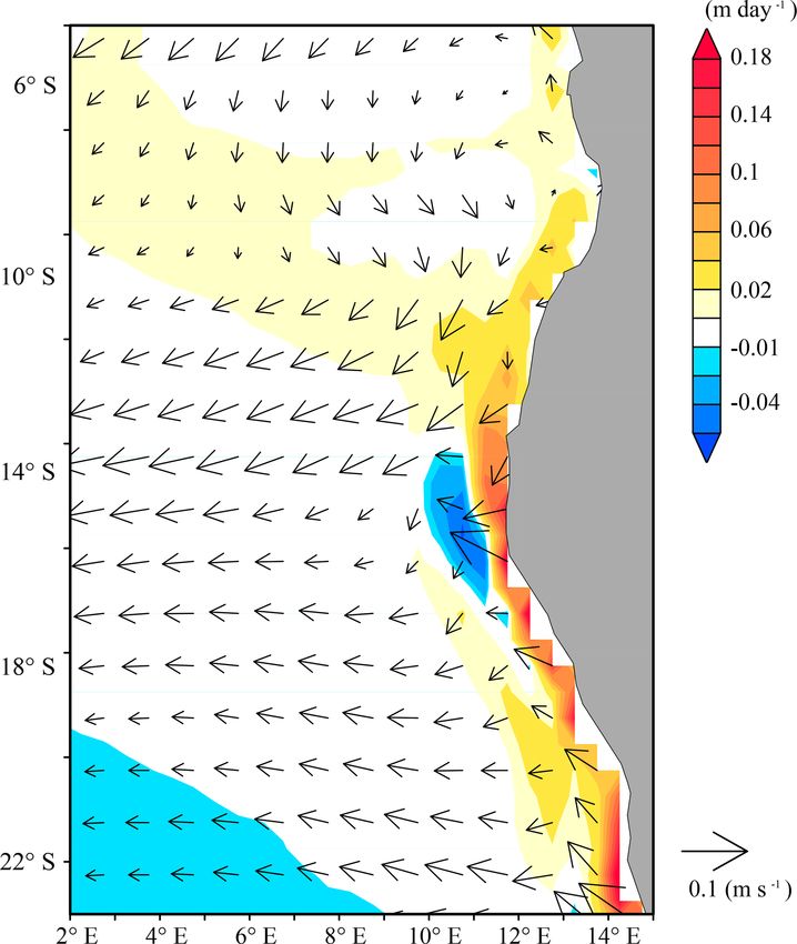
S. Koseki et al.: Frontogenesis of the Angola–Benguela Frontal Zone                                                                   85

Figure 1. (a) Global image of observed 1982–2010 OISST. (b) Annual-mean SST (contour, ◦ C) and its meridional gradient (◦ C per 100 km)
around the ABFZ.

SST-gradient is oriented south–north. The right-hand side of          in the south of the ABFZ (e.g., Morholz et al., 1999). The
Eq. (1) can be written as,                                            shear term can explain the conversion of such a zonal gra-
                                                                dient into meridional gradient. The convergence term repre-
 d ∂θ              ∂ ∂θ          ∂ ∂θ                                 sents strengthening or weakening of the meridional temper-
              =u            +v
 dt ∂y            ∂x  ∂y      ∂y ∂y                               ature gradient by convergence or divergence of meridional
                  ∂ ∂θ         ∂ ∂θ                                   current. The tilting term represents conversion of the vertical
              +w            +
                  ∂z ∂y       ∂t ∂y                                   stratification into meridional gradient by meridional shear of
                  ∂u ∂θ ∂v ∂θ ∂w ∂θ
              =−          −        −                                  vertical velocity.
                  ∂y ∂x ∂y ∂y       ∂y ∂z                              The fourth term is a thermodynamical term due to ex-
                 ∂ ∂θ       ∂θ      ∂θ     ∂θ
              +          +u     +v     +w                             change of heat associated with the turbulent heat flux (surface
                ∂y ∂t       ∂x      ∂y      ∂z                      heat flux is included into w0 θ 0 ; it is the surface boundary con-
                  ∂u ∂θ ∂v ∂θ ∂w ∂θ            ∂ dθ
              =−          −        −        +                         dition). The contribution due to the second-order horizontal
                  ∂y ∂x ∂y ∂y        ∂y ∂z ∂y dt                      diffusion is ignored for simplicity.
and using                                                                Since within the OML the temperature is fairly uniform
                                                                      (cf. Fig. 2 to compare the SST and OML-averaged temper-
dθ    ∂w0 θ 0                                                         ature), we consider the OFGF with the mixed-layer mean
   =−                                                                 quantities. With the approximation that temperature is in-
dt     ∂z
                                                                      dependent of the depth in the OML (e.g., Kazmin and Rie-
we obtain                                                             necker, 1996; Tozuka and Cronin, 2014), Eq. (2) can be ex-

 d ∂θ             ∂u ∂θ ∂v ∂θ                                         pressed as
              =−        −
 dt ∂y            ∂y ∂x ∂y ∂y
                                                                        d ∂θoml

                                                                                             ∂uoml ∂θoml ∂voml ∂θoml
                                                             (2)
                                      !
                ∂w ∂θ    ∂   ∂w 0 θ 0                                                   =−                    −
              −       +    −            .                               dt     ∂y             ∂y ∂x                ∂y  ∂y
                                                                                          ∂(wb + we ) 1θ            ∂ Qs + Qb
                                                                                                                                     (3)
                ∂y ∂z ∂y      ∂z
                                                                                        −                       +                  ,
                                                                                               ∂y          D       ∂y     ρCp D
Here, u, v, and w denote the zonal, meridional, and ver-
tical current velocities, respectively. Equation (2) describes        where the subscript oml indicates the OML-mean quantity
the processes that act to generate or destroy the ocean front.        estimated by
The terms − ∂u   ∂θ     ∂v ∂θ         ∂w ∂θ
              ∂y ∂x , − ∂y ∂y , and − ∂y ∂z are the contributions                  surface
                                                                                    Z
due to the mechanical processes: shear, convergence, and tilt-                 1
                                                                      Aoml =             A · dz,
ing, respectively. The shear term represents conversion of                     D
the zonal temperature gradient into meridional gradient by                          D

zonal current shear. In particular, the cool SST associated           where D denotes the OML depth, i.e., the terms with sub-
with the Benguela upwelling creates a strong zonal gradient           script oml include the changes in the OML implicitly. Al-

www.ocean-sci.net/15/83/2019/                                                                            Ocean Sci., 15, 83–96, 2019
86                                                        S. Koseki et al.: Frontogenesis of the Angola–Benguela Frontal Zone

Figure 2. Climatological seasonal cycle of the temperature (contour) and its meridional gradient averaged between 10 and 12◦ E for (a) SST
of OISST, (b) SST of CFSR, and (c) OML-mean potential temperature of CFSR.

though the horizontal velocity is a function of depth even in            While Eq. (3) is the Lagrangian form of the OFGF, the
the OML, the horizontal mechanical terms in Eq. (3) can be             equation can also be expressed in Eulerian form as below:
written in terms of OML-mean quantities because the pro-
duction is linear in u and v as long as the temperature is in-           ∂ ∂θoml            ∂uoml ∂θoml ∂voml ∂θoml
                                                                                       =−                −
dependent of depth in the OML. Symbols wb , we , 1θ , and D             ∂t    ∂y              ∂y ∂x          ∂y ∂y
                                                                                            |    {z     } |     {z    }
represent the vertical velocity, the entrainment velocity, the                                  SHER           CONF
                                                                                          ∂wb 1θ      ∂

                                                                                                            Qs
                                                                                                                               (4)
temperature jump at the bottom of the OML, and the OML
                                                                                       −          +                + residual .
depth, respectively. According to Moisan and Niller (1998),                                ∂y D      ∂y ρCp D        | {z }
the entrainment velocity at the bottom of the OML is esti-                               | {z } |          {z    }     RESD
                                                                                              TILT           SFLX
mated by

       ∂D                                                              In this equation, the kinematic − ∂w   e 1θ
                                                                                                            ∂y D     and diabatic Qb
we =      + ub · ∇D,
       ∂t                                                              entrainment terms, and the horizontal and vertical advection
                                                                       terms of ∂θoml /∂y, are included in the residual (RESD). Ac-
where ub is the horizontal velocity at the bottom of the OML.          curate estimation of the entrainment terms are not possible
1θ is estimated as the difference between the OML-mean                 from CFSR outputs and the horizontal and vertical advection
temperature and the temperature just below the OML. We                 effects are not related to Lagrangian sources of the frontoge-
use constant values for sea water density, ρ (1000 kg m−3 ),           nesis. In the remainder of this paper, the shear term will be
and isobaric specific heat of sea water, Cp (4200 J kg−1 K−1 ).        referred to as SHER, the confluence as CONF, the tilting as
The vertical
            mixing
                    term is replaced with Qs and Qb , where           TILT, the thermodynamic term as SFLX, and the residual as
Qs = −w θ  0  0     is the surface net heat flux at the top of
                z=0
                                                                       RESD.
the
 OML      (downward is positive in this study) and Qb =                 Note that our climatology is a 29-year mean from 1982
  −w0 θ 0      represents the vertical mixing at the bottom of         to 2010 (the procedure of making daily climatology of tem-
          z=D                                                          perature meridional gradient and OFGF are described in the
the OML, i.e., in the thermocline. We assume that there is             Supplement). However, some years do not have OML data at
no penetration of shortwave radiation beyond the OML to                some grid points around the coastal region. For these grid
deeper ocean layers. Because the vertical turbulent mixing             points, we make the climatology only for available years.
term at the mixed-layer base Qb is represented according               For example, the smallest number in the focusing ABFZ is
to K-profile parameterization in ocean–atmosphere general              16 years at 16.25◦ S.
circulation models (OAGCMs), it will not be explicitly ad-
dressed in this study as it is not possible to estimate it from
the reanalysis outputs.

Ocean Sci., 15, 83–96, 2019                                                                           www.ocean-sci.net/15/83/2019/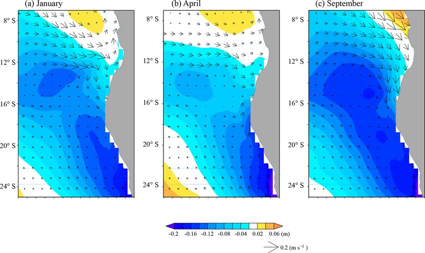
S. Koseki et al.: Frontogenesis of the Angola–Benguela Frontal Zone 87
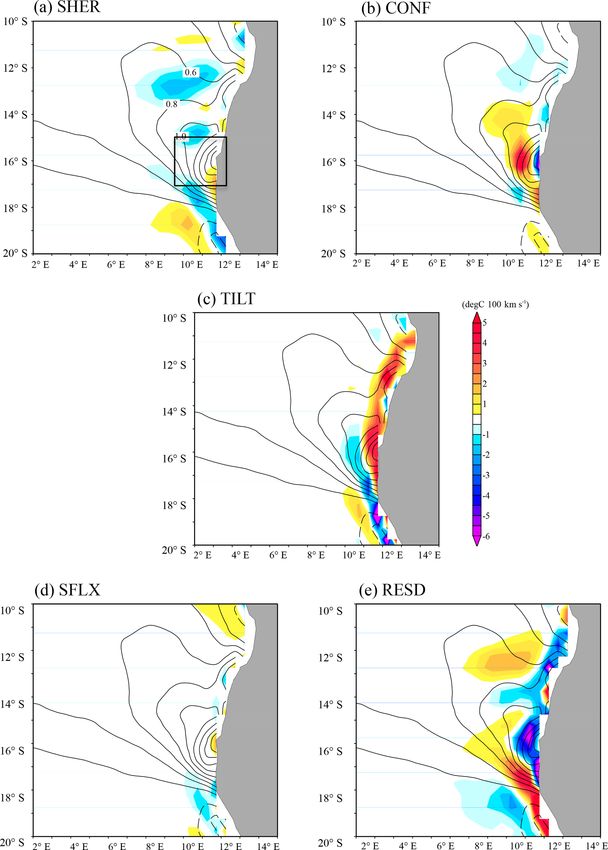
4 Overview of the ABFZ and its seasonal cycle in meridional gradient of the OML-mean temperature. SHER
CFSR data works frontolytically (destroying the front, about −2 ◦ C per
100 km × 10−7 s−1 ) in most parts of the ABFZ, except just
Before the dynamical diagnosis is performed, we provide a near the coast at 17◦ S; although its frontogenetic (generat-
brief overview of the main features of the ABFZ. The max- ing front) contribution is rather weak here (less than 2 ◦ C
imum of the ABFZ (up to 1.4 ◦ C per 100 km) is located at per 100 km × 10−7 s−1 ). CONF has on average an intense
16◦ S just near the coast (Fig. 1b). Figure 2a shows a seasonal frontogenetic contribution to the ABFZ (up to 5 ◦ C per
cycle of the temperature and its meridional gradient obtained 100 km × 10−7 s−1 ), especially offshore around 16◦ S, the
from the satellite product OISST. In this study, the maximum latitude where the ABFZ is centered (Fig. 2). The fronto-
value of the meridional SST gradient is defined as the inten- genetic effect of CONF is consistent with GC2014 (the fron-
sity of the ABFZ. The core (SST meridional gradient exceeds togenesis of the SST front associated with the equatorial At-
1.0 ◦ C per 100 km) of the ABFZ always lies between 17 and lantic cold tongue is due to the confluence of the northern
15◦ S. At the climatological seasonal timescale, the location South Equatorial Current and Guinea Current) and can be
of the ABFZ exhibits a rather weak variability compared to expected because the warm and cold currents meet around
strong interannual variability associated with the Benguela the ABFZ. Note, however, a small zone just near the coast at
Niño events that push the ABFZ southward due to the south- 16◦ S where the CONF is frontolytic. This local frontolytic
ward intrusion of tropical warm water (e.g., Gammelsrød et contribution is overcompensated by a strong frontogenesis
al., 1998; Veitch et al., 2006; Rouault et al., 2017). For in- due to TILT (more than 5 ◦ C per 100 km × 10−7 s−1 on aver-
stance, Rouault et al. (2017) showed that during the Benguela age in the ABFZ core). An elongated frontogenetic zone as-
Niño 2010–2011 the ABFZ displaced southward as far as sociated with TILT is found along the Angolan coast from 17
20◦ S. The intensity of the ABFZ shows a pronounced sea- to 11◦ S and corresponds to the upwelling tongue observed in
sonal cycle: there are two peaks in the strength in April to the Angola Current region (Fig. 3). On the other hand, TILT
May and November to December, respectively. The semi- is frontolytic off the ABFZ (at 17◦ S, 11◦ E) where the down-
annual cycle of the ABFZ will be examined in more detail welling is dominant as shown in Fig. 3. The role of the up-
in the following sections. Figure 2b and c evidence that the welling in the ABFZ development will be analyzed in more
CFSR reanalysis reproduces realistically the annual cycle of detail in Sect. 6.2.
the ABFZ, and that the annual cycle of the corresponding In addition to the mechanical terms, the thermodynami-
OML-mean temperature meridional gradient is representa- cal component also shows some influences on the ABFZ.
tive of the annual cycle of the SST meridional gradient in SFLX works frontogenetically just near the coast at 16◦ S and
terms of both timing and intensity of the two annual peaks. frontolytically south and north from the core of the ABFZ;
This latter result justifies our approach to diagnose the fron- although its contribution is almost negligible compared to
togenesis of the ABFZ with the OML-mean quantities. the mechanical contribution. Annual-mean climatology of
RESD is estimated from Eq. (4) where the left-hand side
(∂θoml /∂y)/∂t is zero for climatology independent of time,
5 Diagnosis on the frontogenesis of the ABFZ
∂uoml ∂θoml ∂voml ∂θoml
In this section, we investigate the frontogenesis of the ABFZ RESD = +
∂y ∂x ∂y ∂y
by diagnostically applying the OFGF described in Sect. 3. ∂wb 1θ ∂ Qs . (5)
Figure 3 illustrates the climatological annual-mean oceanic + −
∂y D ∂y ρCp D
dynamical fields. The southwestward Angola and northwest-
ward Benguela alongshore currents collide just south of the Note that all terms in Eq. (5) are for an annual-mean clima-
ABFZ. Seaward from the ABFZ, a strong westward current tology. On average in the core of the ABFZ, RESD shows a
is detected. An intense upwelling (vertical velocity at the bot- strong frontolytic contribution around the core of the ABFZ
tom of OML exceeding 0.18 m day−1 ) is generated along the (Fig. 4e). On the other hand, frontogenesis is located in the
coast in the Benguela Current region. A local maximum of southern part of the ABFZ. This may be due to, at least partly,
upwelling in the ABFZ (approximately 17◦ S) corresponds vertical mixing at the base of the OML accounted for in
to one of the most vigorous upwelling cells in the region, RESD. In particular, GC2014 showed that for the SST front
namely the Kunene upwelling cell (Kay et al., 2018). Note associated with the equatorial Atlantic cold tongue, the tur-
also a relatively weak downwelling cell (vertical velocity bulent mixing (surface and thermocline heat fluxes) is fron-
down to −0.06 m day−1 ) just seaward from the Kunene up- tolytic.
welling cell.
5.2 Seasonal cycle
5.1 Annual-mean state
In the preceding subsection, we have shown that in terms of
Figure 4 presents the annual-mean climatology of the climatological annual-mean, CONF and TILT of the OFGF
5 forcing or source terms of the OFGF superimposing the were the main sources for the ABFZ generation. Next, we
www.ocean-sci.net/15/83/2019/ Ocean Sci., 15, 83–96, 2019
88                                                        S. Koseki et al.: Frontogenesis of the Angola–Benguela Frontal Zone

                                                                     ABFZ, there is a seasonal cycle of frontogenesis and frontol-
                                                                     ysis in Fig. 5a as the tendency of the ABFZ (green line): two
                                                                     maxima in frontogenesis in March–April and September–
                                                                     October and in frontolysis in May–June and December–
                                                                     February. The tendency of the ABFZ is estimated by Eq. (6).
                                                                        We further analyze the seasonal cycle of the OFGF terms.
                                                                     Similarly to the climatological state in Fig. 4, the contribu-
                                                                     tions of SHER and SFLX are relatively small and do not
                                                                     seem to be responsible for either of the two peaks in the
                                                                     ABFZ annual cycle (not shown). Figure 5b shows the sea-
                                                                     sonal variations of TILT, CONF, and RESD averaged over
                                                                     the same box as the temperature gradients in Fig. 5a. For es-
                                                                     timation of seasonal variation in RESD, the tendency of the
                                                                     meridional gradient is calculated as
                                                                                                  ∂θoml (t+1t)
                                                                     ∂

                                                                              ∂θoml (t)

                                                                                                       ∂y        − ∂θoml∂y
                                                                                                                        (t−1t)
                                                                                              =                                  ,    (6)
                                                                     ∂t         ∂y                           21t

                                                                     where t and 1t denote each time step and difference in time
                                                                     step; in this case, 1t is 1 day (86 400 s). With this tendency
                                                                     at each day, RESD(t) is estimated by

                                                                                        ∂ ∂θoml (t)
                                                                      RESD(t)         =               − SHER(t) − CONF(t)
                                                                                        ∂t     ∂y
                                                                                      −TILT(t) − SFLX(t).
Figure 3. Annual-mean climatological states of OML-mean hori-
zontal current (arrows) and vertical velocity at the bottom of the   From the middle of November to February, the box-averaged
OML (color).                                                         CONF is modestly negative, which is due to the frontolytic
                                                                     effect adjacent to the Angolan coast as shown in Fig. 4b
                                                                     (however, CONF is frontogenetic off the ABFZ). The con-
analyze the annual cycle of the ABFZ and its relationship            tribution of CONF becomes positive from March, although
to the seasonal variations in the OFGF terms. As shown in            its frontogenetic contribution is relatively weak (< 1.0 ◦ C
Fig. 2, the seasonal cycle of the ABFZ exhibits two peaks.           per 100 km × 10−7 s−1 ) until July. From the end of July
Note that if the seasonal cycle is sinusoidal, Eq. (4) implies       CONF starts to increase and reaches its maximum (3.0 ◦ C per
π/2 phase shift between the OFGF and temperature merid-              100 km × 10−7 s−1 ) at the end of August. The frontogenetic
ional gradient. This means that for a semiannual oscillation         contribution of CONF remains strong until the beginning of
the temperature meridional gradient should lag the OFGF by           October but then rapidly decrease to become frontolytic in
approximately 1.5 months.                                            November.
   Figure 5a illustrates the box-mean (10–12◦ E and 17–                 The contribution of TILT to the ABFZ seasonal cycle is
   ◦
15 S) time series of the meridional gradient of temper-              almost always frontogenetic. Close to zero in January, TILT
ature obtained from satellite and reanalysis products (the           is enhanced from February and reaches its maximum value
time series is smoothed by a 11-day mean moving filter).             (3.0 ◦ C per 100 km × 10−7 s−1 ) in March–April. In May–
This box covers the maximum of the ABFZ in each month                June, the frontogenetic effect of TILT gradually decreases
since the meridional location of the ABFZ is almost sta-             (down to 1.0 ◦ C per 100 km × 10−7 s−1 ) until December. The
ble in the climatological seasonal cycle. There is an obvi-          maxima in TILT and CONF correspond to the two periods of
ous semiannual cycle of the ABFZ with maxima in April–               development of the ABFZ at the seasonal timescale: from
May and in November–December, and minima in February–                March to April and from August to October, respectively
March and July–August (see also Fig. 2). The first maximum           (Fig. 5a). This suggests that the two peaks of the ABFZ are
develops rapidly (during 2 months, from March to April),             associated with two different mechanical terms and thus are
whereas the development of the second maximum is some-               due to two different physical processes. On the other hand,
what slower (3 months, from August to October). Figure 5a            the two periods of decay of the ABFZ are consistent with
also evidences that CFSR realistically reproduces the semi-          the periods of weak frontogenetic and/or frontolytic contri-
annual cycle, although the magnitudes of the CFSR merid-             butions of both TILT and CONF (as observed by Mohrholz
ional SST gradient are generally slightly stronger with re-          et al., 1999) in December–February and June–July, respec-
spect to OISST. Corresponding to the annual cycle of the             tively.

Ocean Sci., 15, 83–96, 2019                                                                                 www.ocean-sci.net/15/83/2019/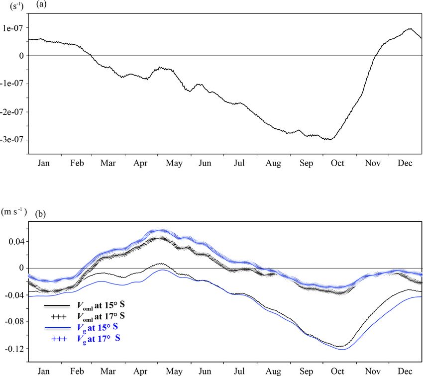
S. Koseki et al.: Frontogenesis of the Angola–Benguela Frontal Zone                                                       89

Figure 4. Annual-mean climatology of each term in OFGF. Contour is annual-mean climatology of meridional gradient of OML-mean
potential temperature of CFSR (◦ C per 100 km). The black box in (a) is the ABFZ used for the analysis in this study.

   In addition, RESD is almost always frontolytic               estimation, the semiannual cycle of the ABFZ is explained
with a relatively large oscillation (0.0 to −5.0 ◦ C per        by the combination of TILT and CONF.
100 km × 10−7 s−1 ) as shown in Fig. 5b. In particular, the
frontolytic effect due to RESD is stably strong (around
−3.0 ◦ C per 100 km × 10−7 s−1 ) from May–August when
                                                                6   Discussion
the ABFZ becomes weakened and frontogenetic effects
due to CONF and TILT are relatively weak (Fig. 5a and b).
                                                                The previous section showed that the two periods of devel-
In contrast with TILT and CONF, RESD does not exhibit
                                                                opment of the ABFZ in March–April and August–October
a clear signal of semiannual cycle, but rather an annual
                                                                were due, to a large extent, to the contribution of TILT and
cycle. We thus can conclude that in terms of a first-order
                                                                CONF, respectively. In this section, we investigate what com-

www.ocean-sci.net/15/83/2019/                                                                   Ocean Sci., 15, 83–96, 2019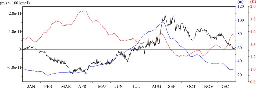
90                                                     S. Koseki et al.: Frontogenesis of the Angola–Benguela Frontal Zone

Figure 5. Box-mean (17–15◦ S and 10–12◦ E) time series of (a) meridional gradient of temperature (black: OISST, red: SST of CFSR,
and blue: OML-temperature of CFSR) and (b) TILT (magenta), CONF (green), SHER (cyan), SFLX (red), and RESD (black). Eleven-day
running means are shown for all time series.

ponents are responsible for the corresponding peaks in TILT        ability induces the geostrophic current, which can contribute
and CONF.                                                          to the current system around the ABFZ. Therefore, here we
                                                                   also focus on the SSH and corresponding geostrophic cur-
6.1   Meridional confluence                                        rent. Figure 6b illustrates the annual cycle of the OML-mean
                                                                   meridional current and meridional component of geostrophic
                                                                   current estimated from SSH at 15◦ S (north of the core of
CONF represents changes in the meridional temperature gra-
                                                                   the ABFZ) and 17◦ S (south of the core of the ABFZ) aver-
dient associated with ocean dynamics of convergence or di-
                                                                   aged between 10 and 12◦ E. At 15◦ S the OML-mean merid-
vergence of meridional current, ∂voml /∂y. Figure 6a presents
                                                                   ional current is southward all year round, except for the be-
the annual cycle of ∂voml /∂y averaged over the ABFZ. In
                                                                   ginning of May when a weak northward flow is observed.
the ABFZ, the meridional current is almost always conver-
                                                                   The maximum southward meridional velocity occurs in Oc-
gent except for weak divergence from November to Jan-
                                                                   tober (−0.12 m s−1 ). At 17◦ S the OML-mean meridional
uary. The convergence of the meridional current is maximum
                                                                   current is northward in March–June and shows a biannual
from August to mid-October (up to −3.0 × 10⁻⁷ s−1 ) and is
                                                                   peak of southward current in January to mid-February and
rapidly weakened during November. The seasonal fluctua-
                                                                   October indicating intrusion of tropical warm water to the
tions in the convergence are associated with changes in inten-
                                                                   ABFZ (e.g., Rouault, 2012). Figure 6b clearly evidences that
sity and meridional extension of the southward Angola Cur-
                                                                   the region between 17 and 15◦ S is expected to be conver-
rent and northward Benguela Current that meet in the ABFZ.
                                                                   gent. The most convergent period is in September–October
Around the ABFZ, an area of lower SSH is formed, asso-
                                                                   when the CONF contribution to frontogenesis is the largest
ciated with the Angola Dome (the cold dome identified by
                                                                   as shown in Fig. 5b. Another relatively strong convergent pe-
Mazeika, 1967), which shows a pronounced seasonal cycle
                                                                   riod is from April to June when the meridional current is
(e.g., Doi et al., 2007). Such well-organized SSH spatial vari-

Ocean Sci., 15, 83–96, 2019                                                                    www.ocean-sci.net/15/83/2019/
S. Koseki et al.: Frontogenesis of the Angola–Benguela Frontal Zone 91
rather northward at 17◦ S and close to zero at 15◦ S. The around the ABFZ more in August–September than in March–
period of weak convergence or divergence, from Decem- April.
ber to February, corresponds to frontolytic contribution of The OML depth has extrema in August–September
CONF (Fig. 5b). Figure 6b evidences that the OML-mean (around 100 m) and from January–April (around 20 m) in-
meridional current can be explained, to a large extent, by the dicating the seasonal cycle of solar insolation forcing and
geostrophic surface current. While a large part of the merid- wind-driven mixing. Also, the intensity of the thermocline
ional current and its seasonal cycle around the ABFZ is ex- shows a strong stratification from March to May (2 ◦ C) and
plained by geostrophic current associated with the SSH to weak stratification from September to November (1.2 ◦ C).
the northwest of the ABFZ, there are some differences be- From March to May TILT is the most dominant frontoge-
tween voml and vg . These differences are due to the Ekman netic source because the OML is the shallowest (20–30 m),
and ageostrophic currents. the stratification is the strongest (temperature jump in the
The spatial distributions of the climatological monthly- thermocline up to 2.0 K), and the shear of vertical veloc-
mean SSH and surface geostrophic current in January, April, ity ∂wb /∂y is strongly negative. The shallow OML and
and September are shown in Fig. 7. Two local minima of strong stratification can amplify the tilting effect due to
SSH are observed: one along the coast in the Benguela sys- ∂wb /∂y. Conversely, TILT is weakly frontolytic from August
tem and one west of the ABFZ (centered at 14◦ S and 6◦ E). to September when the OML depth is deepened (∼ 100 m),
The latter is associated with the Angola Dome (e.g., Doi et the stratification is weak (1.2 K), and ∂wb /∂y is positive. Fig-
al., 2007) and a strong cyclonic geostrophic flow reaching ure S1c and d shows the differences in OML depth and ocean
the ABFZ. The geostrophic current generally generates the stratification between March–April and August–September.
convergence in the ABFZ (Fig. 6a). However, in January an Shallower OML and stronger stratification can be seen ev-
intense divergence is generated due to the strong southward erywhere around the ABFZ. Therefore, effects of both pos-
ageostrophic current along the coast (Fig. 7a). In April, when itive and negative ∂wb /∂y are reduced and consequently,
CONF is modestly frontogenetic (Fig. 5b), the Angola Dome the contribution of TILT is quite weak in August–September
and associated geostrophic flow are diminished (Fig. 7b) and (Fig. 5b).
a main source of convergence can thus be attributed to the
northward Benguela Current that penetrates into the ABFZ
as far as 16◦ S. In September, although the low SSH sits in the 7 Concluding remarks
south of the ABFZ as in April, the Angola Dome is signifi-
In this study we investigated the processes controlling the
cantly developed to be related to a strong geostrophic current
ABFZ evolution based on a first-order estimation of an ocean
resulting in a strong southward Angola Current intruding into
frontogenetic function (OFGF) applied to the ocean mixing
the ABFZ along the Angolan coast. The northward Benguela
layer (OML) derived from the CFSR reanalysis. The OFGF
Current is relatively weak in September compared to that in
represents the temporal evolution of the meridional mixed-
April. Thus, the maximum CONF in September is due to the
layer temperature gradient and contains three mechanical
strong southward Angola Current.
terms (shear, convergence and tilting) and one thermody-
namical term. The residual term accounts for, in particular,
6.2 Tilting
vertical mixing at the bottom of the OML (which is based
on parameterization of turbulence, i.e., highly nonlinear pro-
TILT is the second main contributor to generate the ABFZ
cesses), entrainment velocity, and horizontal or vertical ad-
especially in March to May as shown in Figs. 4 and 5. In
vection of the meridional temperature gradient. An analysis
a first approximation, TILT results from the meridional gra-
of the annual mean OFGF suggests that the confluence effect
dient of vertical motion ∂wb /∂y convoluted with the ther-
(CONF) due to southward Angola Current (warm) and north-
mocline stratification (e.g., Eq. 4). Here, we explore more
ward Benguela Current (cold) is dominantly frontogenetic
details of upwelling in the ABFZ. The annual cycle of these
over the offshore part of the ABFZ, although it has a local
two components averaged over the box 12–10◦ E and 17–
frontolytic effect just near the coast at 16◦ S. The tilting ef-
15◦ S (Fig. 8) points out the negative ∂wb /∂y and the posi-
fect (TILT) related to the coastal upwelling regime is another
tive stratification from January to August, respectively. This
main contributor to frontogenesis. Around the ABFZ, intense
configuration leads to frontogenesis through the TILT term
Ekman transport divergence is generated by wind stress curl
(Fig. 5b). From August to December, ∂wb /∂y changes sign
(Fig. S2). This Ekman divergence induces upward motion in
and the stratification becomes weaker; that explains why the
the Ekman layer. Interestingly, the Ekman divergence due to
TILT term is frontolytic (especially in September) and its
the zonal wind stress is also an important contributor to the
magnitude is weaker compared to January–August because
vertical velocity in the ABFZ. The contributions of the shear
of a weaker stratification (smaller vertical gradient in tem-
(SHER) and surface heat flux (SFLX) terms are rather negli-
perature). Negative ∂wb /∂y can be seen in both March–April
gible, while the residual (RESD) term represents a main fron-
and August–September around the ABFZ in Fig. S1a and b
tolytic source.
in the Supplement, but positive ∂wb /∂y are also generated
www.ocean-sci.net/15/83/2019/ Ocean Sci., 15, 83–96, 201992 S. Koseki et al.: Frontogenesis of the Angola–Benguela Frontal Zone
Figure 6. Time series of (a) averaged over (17–15◦ S and 10–12◦ E) and (b) OML-mean meridional current velocity (black) and geostrophic
meridional current velocity estimated from sea surface height (blue) at 15◦ S (solid line) and 17◦ S (+ mark) averaged between 10 and 12◦ E.
All variables are filtered by a moving 11-day window.
Climatological seasonal evolution of the ABFZ has a on the development of the ABFZ maximum in March–April.
well-pronounced semiannual cycle with two maxima of the On the other hand, the importance of the OML depth for the
SST meridional gradient, in April–May and November– thermodynamical term was suggested for frontogenesis in a
December, and two minima, in February–March and July– SST front associated with western boundary current (Tozuka
August. We showed that the two maxima of the ABFZ were and Cronin, 2014; Tozuka et al., 2018). The annual maxi-
associated with two different mechanical terms and due to mum of CONF in September–October is related to an inten-
two different physical processes. The development of the sified southward Angola Current that seems to be induced by
first ABFZ maximum during March–April is mainly ex- an approximately cyclonic geostrophic flow associated with
plained by the strong contribution of TILT to frontogenesis, the development of the Angola Dome (e.g., Doi et al., 2007).
while the development of the second ABFZ maximum dur- However, the geostrophic current is not completely consis-
ing September–October is due to the frontogenetic contribu- tent with the OML-mean current. The difference can be at-
tion of CONF. TILT is associated with the meridional gradi- tributed to the Ekman transport and ageostrophic component.
ent of the vertical velocity. The annual maximum of TILT in A relatively smaller contribution of CONF to frontogenesis
March–April is due, to a large extent, to the combination of is also observed in April and is due to the intrusion of the
the maximum stratification (1θ), shallow OML depth (D), northward Benguela Current to the ABFZ during this period.
and negative ∂wb /∂y during this period. Indeed, in OFGF the Most CGCMs fail to reproduce realistic SST fields and
ratio 1θ
D represents the efficiency by which the meridional ABFZ locations with respect to climatology. Among other
gradient of the coastal upwelling velocity can lead to the causes, this can be due to a poor representation of regional
change of the ABFZ intensity. Although the OML depth also climate variables in CGCMs (such as upwelling-favorable
modulates the surface heat flux contribution to the OFGF, the wind, wind drop off, and consequently near-coastal wind
thermodynamical term does not show any significant impact curl, alongshore stratification, and OML depth (e.g., Xu et
Ocean Sci., 15, 83–96, 2019 www.ocean-sci.net/15/83/2019/S. Koseki et al.: Frontogenesis of the Angola–Benguela Frontal Zone 93
Figure 7. Monthly mean SSH (color) and geostrophic current (arrows) for (a) January, (b) April, and (c) September.
Figure 8. Time series of the area-averaged meridional gradient of the vertical velocity at the bottom of OML (black), OML depth (blue),
intensity of upper-ocean thermocline stratification (red) over 17–15◦ S and 10–12◦ E. All variables are filtered by a moving 11-day window.
al., 2014; Koseki et al., 2018; Goubanova et al., 2018), which Although the present study focused on the climatological
directly impact the two main frontogenesis terms (CONF and state of the ABFZ and its seasonal cycle, the intensity and the
TILT). The OFGF proposed in the present study can thus be location of the ABFZ exhibits a strong interannual variabil-
an appropriate tool to diagnose the performance of CGCMs ity (e.g., Mohrholz et al., 1999; Rouault et al., 2017). Further
in the ABFZ and more generally in frontal zones. This study investigation on how the contributions of the OFGF are mod-
shows that diagnoses developed for mesoscale studies are ified in the case of the Benguela Niño/Niña would provide
valuable for climate studies and can help to identify the ori- further insight into the dynamics of the southeastern tropical
gin of biases that affect ocean general circulation models Atlantic and sources of the CGCMs bias that have been sug-
(OGCMs). gested to develop as interannual warm events (e.g., Xu et al.,
2014).
www.ocean-sci.net/15/83/2019/ Ocean Sci., 15, 83–96, 201994 S. Koseki et al.: Frontogenesis of the Angola–Benguela Frontal Zone
Effects of the turbulent mixing and the effect due to the en- grant no. 648982). Katerina Goubanova was also supported by
trainment velocity at the mixed-layer base on frontogenesis FONDECYT (grant 1171861).
were accounted for by the residual of the frontogenetic func-
tion. An accurate quantification of these effects requires us- Edited by: John M. Huthnance
ing simulations of a higher resolution ocean model for which Reviewed by: two anonymous referees
the output of the temperature tendency due to those processes
are available. According to Giordani and Caniaux (2014),
the vertical mixing is also a large contributor to the fron-
togenesis. However, by destroying the balance between the References
mass and circulation fields, the assimilation procedure in-
duces spurious effects on the entrainment processes, which Astudillo, O., Dewitte, B., Mallet, M., Frappart, F., Rutllant,
justifies that this process was included in the residual term J. A., Ramos, M., Bravo, L., Goubanova, K., and Illig, S.:
RESD. These are the main limitations of this study because Surface winds off Peru-Chile: Observing closer to the coast
diapycnal mixing is often an important term of the oceanic from radar altimetry, Remote Sens. Environ., 191, 179–196,
upper-layers heat budget, which is tightly coupled with ver- https://doi.org/10.1016/j.rse.2017.01.010, 2017.
Auel, H. and Verheye, H. M.: Hypoxia tolerance in the copepod
tical motions (Giordani et al., 2013). A more comprehensive
Calanoides carinatus and the effect of an intermediate oxygen
understanding of this term would be valuable to estimate the minimum layer on copecod vertical distribution in the northern
performance of CGCMs in the ABFZ and more generally in Bengulea Current upwelling system and the Angola-Benguela
coastal upwelling zones. Front, J. Exp. Mar. Biol. Ecol., 352, 234–243, 2007.
Chavez, F. P. and Messié, M.: A comparison of eastern boundary
upwelling ecosystem, Prog. Oceanogr., 83, 80–96, 2009.
Data availability. The CFSR reanalysis data (Saha et al., 2010) Chen, Z., Yan, X.-H., Jp, Y.-H., Jiang, L., and Jiang, Y.: A study
used in this study can be downloaded from https://climatedataguide. of Bengulea upwelling system using different upwelling indices
ucar.edu/climate-data/climate-forecast-system-reanalysis-cfsr. The derived from remotely sensed data, Cont. Shelf Res., 45, 27–33,
data of OISST (Reynolds, et al., 2007) are available at https://www. 2012.
ncdc.noaa.gov/oisst. Colberg, F. and Reason, C. J. C.: A model study of
the Angola Benguela Frontal Zone: Sensitivity to at-
mospheric forcing, Geophys. Res. Lett., 33, L19608,
Supplement. The supplement related to this article is available https://doi.org/10.1029/2006GL027463, 2006.
online at: https://doi.org/10.5194/os-15-83-2019-supplement. Colberg, F. and Reason, C. J. C.: A model investigation of internal
variability in the Angola Benguela Forntal Zone, J. Geophys.
Res., 112, C07008, https://doi.org/10.1029/2006JC003920,
Author contributions. SK derived the ocean frontogenetic function 2007.
(OFGF) by discussing with HG and KG and improved the OFGF. Dinniman, M. S. and Rienecker, M. M.: Frontogenesis in the North
SK performed the main analysis of the data and all authors con- Pacific Ocean Frontal Zones-A Numerical Simulation, J. Phys.
tributed to the interpretation of the results and discussion. SK wrote Oceanogr., 29, 537–559, 1999.
a first draft and HG and KG improved the draft extensively with Doi, T., Tozuka, T., Sasaki, H., Masumoto, Y., and Yamagata,
constructive and critical comments on the draft. T.: Seasonal and interannual variations of oceanic conditions
in the Angola Dome, J. Phys. Oceanogr., 37, 2698–2713,
https://doi.org/10.1175/2007JPO3552.1, 2007.
Fennel, W., Junker, T., Schmidt, M., and Mohrholz, V.: Response of
Competing interests. The authors declare that they have no conflict
the Benguela upwelling system to spatial variations in the wind
of interest.
stress, Cont. Shelf Res., 45, 65–77, 2012.
Florenchie, P., Lutjeharms, J. E., Reason, C. J. C., Masson,
S., and Rouault, M.: The source of Benguela Ninos in
Acknowledgements. We greatly appreciate two anonymous the South Atlantic Ocean, Geophys. Res. Lett., 30, 1505,
reviewers for their constructive and helpful comments. Also, https://doi.org/10.1029/2003GL017172, 2003.
we would like to express our appreciation to Kunihiro Aoki Gammelsrød, T., Bartholomae, C. H., Boyer, D. C., Filipe, V.
in the University of Tokyo for his constructive discussion in L. L., and O’Toole, M. J.: Intrusion of warm surface water
the initial stage of this study. We also thank Guy Caniaux along the Angolan-Namibian coast in February–March 1995:
in Météo-France for their helpful discussions. We used the the 1995 Benguela Nino, S. Afr. J. Marine Sci., 19, 41–56,
2012Rb versions of the MATLAB software package provided https://doi.org/10.2989/025776198784126719, 1998.
by MathWorks, Inc., (http://www.mathworks.com, last access: Giordani, H. and Caniaux, G.: Sensitivity of cyclogenesis to sea
13 August 2018) and Grid Analysis and Display System (GrADS, surface temperature in the Northwestern Atlantic, Mon. Weather
http://cola.gmu.edu/grads/, last access: 30 November 2018) to Rev., 129, 1273–1295, 2001.
compute each dataset and create figures. Shunya Koseki has Giordani, H. and Caniaux, G.: Diagnosing vertical motion
received funding from the EU FP7/2007–2013 under grant in the Equatorial Atlanitc, Ocean Dynam., 61, 1995–2018,
agreement no. 603521 (EU-PREFACE) and STERCP (ERC, https://doi.org/10.1007/s10236-01-0467-7, 2011.
Ocean Sci., 15, 83–96, 2019 www.ocean-sci.net/15/83/2019/S. Koseki et al.: Frontogenesis of the Angola–Benguela Frontal Zone 95 Giordani, H., Caniaux, G., and Voldoire, A.: Intraseasonal mixed- Lutz, K., Jacobeit, J., and Rathmann, J.: Atlantic warm and cold layer heat budget in the equatorial Atlantic during the cold water events and impact on African west coast precipitation, Int. tongue development 2006, J. Geophys. Res., 118, 650–671, J. Climatol., 35, 128–141, 2015. https://doi.org/10.1029/2012JC008280, 2013. Manhique, A. J., Reason, C. J. C., Silinto, B., Zucula, J., Giordani, H. and Caniaux, G.: Lagrangian sources of frontogenesis Raiva, I., Congolo, F., and Mavume, A. F.: Extreme rain- in the equatorial Atlantic front, Clim. Dynam., 43, 3147–3162, fall and floods in southern Africa in January 2013 and https://doi.org/10.1007/s00382-014-2293-3, 2014. associated circulation patterns, Nat. Hazards, 77, 679–691, Goubanova, K., Illig, S., Machu, E., Garcon, V., and De- https://doi.org/10.1007/s11069-015-1616-y, 2015. witte, B.: SST subseasonal variability in the central Mazeika, P. A.: Thermal domes in the eastern tropical Atlantic Benguela upwelling system as inferred from satellite ob- Ocean, Limnol. Oceanogr., 12, 537–539, 1967. servation (1999–2009), J. Geophys. Res., 118, 4092–4110, Mohrholz, V., Schmidt, M., Lutjeharms, J. R. E., and John, H.-C. https://doi.org/10.1002/jgrc.20287, 2013. H.: Space-time behavior of the Angola-Benguela Frontal Zone Goubanova, K., Sanchez, G., E., Frauen, C., and Voldoire A.: Role during the Benguela Nino of April 1999, Int. J. Remote Sens., 25, of remote and local wind stress forcing in the development of 1400, https://doi.org/10.1080/01431160310001592265, 2004. the warm SST errors in the southeastern tropical Atlantic in a Moisan, J. R. and Niler, P. P.: The Seasonal Heat Budget of the coupled high-resolution model, Clim. Dynam., 2018. North Pacific: Net Heat Flux and Heat Storage Rate (1950– Griffies, S. M., Harrison, M. J., Pacanowski, R. C., and Rosati, A.: 1990), J. Phys. Oceanogr., 28, 401–421, 1998. Technical guide to MOM4, GFDL Ocean Group Technical Re- NCAR/UCAR Climate Data Guide: Climate Forecast System Re- port No. 5, 337 pp., available at: https://www.gfdl.noaa.gov/-fms analysis (CFSR), available at: https://climatedataguide.ucar.edu/ (last access: 15 November 2018), 2004. climate-data/climate-forecast-system-reanalysis-cfsr, last ac- Hanshingo, K. and Reason, C. J. C.: Modelling the atmospheric re- cess: 7 February 2019. sponse over southern Africa to SST forcing in the southeast trop- NOAA: Optimum Interpolation Sea Surface Temperature (OISST), ical Atlantic and southwest subtropical Indian Oceans, Int. J. Cli- available at: https://www.ncdc.noaa.gov/oisst, last access: 7 matol., 29, 1001–1012, https://doi.org/10.1002/joc.1919, 2009. February 2019. Hastenrath, S. and Lamb, P.: On the dynamics and climatology of Pfeifroth, U., Hollmann, R., and Ahrens, B.: Cloud Cover Diurnal surface flow over the equatorial oceans, Tellus, 30, 436–448, Cycles in Satellite Data and Regional Climate Model Simula- 1978. tions, Meteorologische Z., 21, 551–560, 2012. Hirst, A. C. and Hastenrath, S.: Atmopshere-Ocean Mechanisms Reynolds, R. W., Smith, T. M., Liu, C., Chelton, D. B., Casey, K. of Climate Anomalies in the Angola-Tropical Atlantic Sector, J. S., and Schlax, M. G.: Daily High-Resolution-Blended Analyses Phys. Oceanogr., 13, 1146–1157, https://doi.org/10.1175/1520- for Sea Surface Temperature, J. Clim., 20, 5473–5496, 2007. 0485(1983)0132.0.CO;2, 1983. Rouault, M., Florenchie, P., Fauchereau, N., and Reason, Junker, T., Schmidt, M., and Mohrholz, V.: The relation of wind C. J. C.: South east tropical Atlantic warm events and stress curl and meridional transport in the Benguela upwelling southern African rainfall, Geophys. Res. Lett., 30, 8009, system, J. Mar. Res., 143, 1–6, 2015. https://doi.org/10.1029/2002GL014840, 2003. Junker, T., Mohrholz, V., Siegfired, L., and van der Plas, A.: Sea- Rouault, M.: Bi-annual intrusion of tropical water in the north- sonal to interannual variability of water mass characteristics and ern Benguela upwelling, Geophys. Res. Lett., 39, L12606, current on the Namibian shelf, J. Mar. Syst., 165, 36–46, 2017. https://doi.org/10.1029/2012GL052099, 2012. Kay, E., Eggert, A., Flohr, A., Lahajnar N., Nausch, G., Nuemann, Rouault, M., Illig, S., Lübbecke, J., and Koungue, R. A., Rixen, T., Schmidt, M., Van der Pla, A., and Wasmund, N.: A. I.: Origin, development and demise of the 2010– Biogeochemical processes and turnover rates in the Northern 2011 Benguela Niño, J. Mar. Syst., 188, 39–48, Benguela Upwelling System, J. Mar. Syst., 188, 63–80, 2018. https://doi.org/10.1016/j,jmarsys.2017.07.007, 2018. Kazmin, A. S. and Rienecker, M. M.: Variability and forntogenesis Saha, S., Moorti S., Pan H.-L., Wu X., Wang, J., Nadiga, S., Tripp, in the large-scale oceanic frontal zones, J. Geophys. Res., 101, P., Kistler, R., Woollen, J., Behringer, D., Liu, H., Stokes, D., 907–921, 1996. Grumbine, R., Gayno, G., Wang, J., Hou, Y.-T., Chuang, H., Keyser, D., Reeder, M. J., and Reed, R. J.: A Generalization of Pet- Juang, H.-M. H., Sela, J., Iredell, M., Treadon, R., Kleist, D., terssens’s Frontogenesis Function and Its Relation to the Forcing Van Delst, P., Keyser, D., Derber, J., Ek, M., Meng, J., Wei, of Vertical Motion, Mon. Weather Rev., 116, 762–780, 1988. H., Yang, R., Lord, S., van den Dool, H., Kumar, A., Wang, Klein S. A. and Hartmann, D. L.: The Seasonal Cycle of Low Strat- W., Long, C., Chelliah, M., Xue, Y., Huang, B., Schemm, J.-K., iform Clouds, J. Clim., 6, 1587–1606, 1993. Ebisuzaki, W., Lin, R., Xie, P., Chen, M., Zhou, S., Higgins, W., Koseki, S., Keenlyside, N., Demissie, T., Toniazzo, T., Counillon, Zou, C.-Z., Liu, Q., Chen, Y., Han, Y., Cucurull, L., Reynolds, R. F., Bethke, I., Ilicak, M., and Shen, M.-L.: Causes of the large W., Rutledge, G., and Goldberg, M.: The NCEP Climate Fore- warm SST bias in the Angola-Benguela Frontal Zone in the cast System Reanalysis, B. Am. Meteorol. Soc., 91, 1015–1058, Norwegian Earth System Model, Clim. Dynam., 50, 4651–4670, https://doi.org/10.1175/2010BAMS3001.1, 2010. https://doi.org/10.1007/s00382-017-3896-2, 2018. Santos, F., Gomez-Gesteria, M., deCastro, M., and Alvarez, I.: Dif- Kopte, R., Brandt, P., Dengler, M., Tchipalanga, P. C. M., ferences in coastal and oceanic SST trends due to the strength- Macueria, M., and Ostrowski, M.: The Angola Cur- ening of coastal upwelling along the Benguela current system, rent: Flow and hydrographic characteristic as observed Cont. Shelf Res., 34, 79–86, 2012. at 11◦ S, J. Geophys. Res.-Oceans, 122, 1177–1189, Tozuka, T. and Cronin, M. G.: Role of mixed layer depth in surface https://doi.org/10.1002/2016JC012374, 2017. frontogenesis: The Agulhas Return Current front, Geophys. Res. www.ocean-sci.net/15/83/2019/ Ocean Sci., 15, 83–96, 2019
96                                                        S. Koseki et al.: Frontogenesis of the Angola–Benguela Frontal Zone

  Lett., 41, 2447–2453, https://doi.org/10.1002/2014GL059624,         Xu Z., Chang, P., Richter, I., Kim, W., and Tang, G.: Diagnos-
  2014                                                                  ing southeast tropical Atlantic SST and ocean circulation bi-
Tozuka, T., Ohishi, S., and Cronin, M. G.: A metric for surface         ases in the CMIP5 ensemble, Clim. Dynam., 43, 3123–3145,
  heat flux effect on horizontal sea surface temperature gradients,     https://doi.org/10.1007/s00382-014-2247-9, 2014.
  Clim. Dynam., 51, 547–561, https://doi.org/10.1007/s00382-          Zuidema, P. et al.: Challenges and Prospects for Reducing Coupled
  017-3940-2, 2018.                                                     Climate Model SST Biases in the Eastern Tropical Atlantic and
Veitch, J. A., Florenchie, P., and Shillington, F. A.: Sea-             Pacific Oceans: The US CLIVAR Eastern Tropical Oceans Syn-
  sonal and interannual fluctuations of the Angola-Benguela             thesis Working Group, B. Amer. Meteorol. Soc., 97, 2305–2328,
  Frontal Zone (ABFZ) using 4.5 km resolution satellite im-             https://doi.org/10.1175/BAMS-D-15-00274.1, 2016.
  agery from 1982 to 1999, Int. J. Remote Sens., 27, 987–998,
  https://doi.org/10.1080/01431160500127914, 2006.
Vizy, E. K., Cook, K. H., and Sun, X.: Decadal change of the
  south Atlantic ocean Angola-Benguela forntal zone since 1980,
  Clim. Dynam., 51, 3251–3273, https://doi.org/10.1007/s00382-
  018-4077-7, 2018.

Ocean Sci., 15, 83–96, 2019                                                                         www.ocean-sci.net/15/83/2019/
You can also read