Polarization and Fake News: Early Warning of Potential Misinformation Targets - arXiv
←
→
Page content transcription
If your browser does not render page correctly, please read the page content below
Polarization and Fake News: Early Warning of Potential
                                        Misinformation Targets

                                        MICHELA DEL VICARIO, IMT School for Advanced Studies Lucca, Italy
                                        WALTER QUATTROCIOCCHI, Ca’ Foscari University of Venice, Italy
arXiv:1802.01400v1 [cs.SI] 5 Feb 2018

                                        ANTONIO SCALA, ISC-CNR Sapienza University of Rome, Italy
                                        FABIANA ZOLLO, Ca’ Foscari University of Venice, Italy
                                        Users polarization and confirmation bias play a key role in misinformation spreading on online social media.
                                        Our aim is to use this information to determine in advance potential targets for hoaxes and fake news. In
                                        this paper, we introduce a general framework for promptly identifying polarizing content on social media
                                        and, thus, “predicting” future fake news topics. We validate the performances of the proposed methodology
                                        on a massive Italian Facebook dataset, showing that we are able to identify topics that are susceptible to
                                        misinformation with 77% accuracy. Moreover, such information may be embedded as a new feature in an
                                        additional classifier able to recognize fake news with 91% accuracy. The novelty of our approach consists in
                                        taking into account a series of characteristics related to users behavior on online social media, making a first,
                                        important step towards the smoothing of polarization and the mitigation of misinformation phenomena.
                                        Additional Key Words and Phrases: social media, fake news, misinformation, polarization, classification

                                        1   INTRODUCTION
                                        As of the third quarter of 2017, Facebook had 2.07 billion monthly active users [1], leading the
                                        rank of most popular social networking sites in the world. In the meantime, Oxford Dictionaries
                                        announced “post-truth” as the 2016 international Word of the Year [2]. Defined as an adjective
                                        “relating to or denoting circumstances in which objective facts are less influential in shaping public
                                        opinion than appeals to emotion and personal belief”, the term has been largely used in the context
                                        of the Brexit and Donald Trump’s election in the United States and benefited from the rise of
                                        social media as news source. Indeed, Internet changed the process of knowledge production in an
                                        unexpected way. The advent of social media and microblogging platforms has revolutionized the
                                        way users access content, communicate and get informed. People can access to an unprecedented
                                        amount of information –only on Facebook more than 3M posts are generated per minute [3]–
                                        without the intermediation of journalists or experts, thus actively participating in the diffusion as
                                        well as the production of content. Social media have rapidly become the main information source
                                        for many of their users: over half (51%) of US users now get news via social media [4]. However,
                                        recent studies found that confirmation bias –i.e., the human tendency to acquire information
                                        adhering to one’s system of beliefs– plays a pivotal role in information cascades [5]. Selective
                                        exposure has a crucial role in content diffusion and facilitates the formation of echo chambers
                                        –groups of like-minded people who acquire, reinforce and shape their preferred narrative [6, 7]. In
                                        this scenario, dissenting information usually gets ignored [8], thus the effectiveness of debunking,
                                        fact-checking and other similar solutions turns out to be strongly limited.
                                        The authors acknowledge financial support from IMT/Extrapola Srl project. The funders had no role in study design, data
                                        collection and analysis, decision to publish, or preparation of the manuscript.
                                        Authors’ addresses: Michela Del Vicario, IMT School for Advanced Studies Lucca, Piazza S. Ponziano, 6, Lucca, 55100, Italy;
                                        Walter Quattrociocchi, Ca’ Foscari University of Venice, Via Torino, 155, 30172, Venice, Italy; Antonio Scala, ISC-CNR
                                        Sapienza University of Rome, Via dei Taurini, 19, 00185, Rome, Italy; Fabiana Zollo, Ca’ Foscari University of Venice, Via
                                        Torino, 155, 30172, Venice, Italy.

                                        ©
:2 M. Del Vicario et al. Since 2013 the World Economic Forum (WEF) has been placing the global danger of massive digital misinformation at the core of other technological and geopolitical risks [9]. Hence, a fundamental scientific challenge is how to support citizens in gathering trustworthy information to participate meaningfully in public debates and societal decision making. However, attention should be paid: since the problem is complex, solutions could prove to be wrong and disastrous. For instance, relying on machine learning algorithms alone (and scientists behind) to separate the truth from the false is naïf and dangerous, and might have severe consequences. As far as we know, misinformation spreading on social media is directly related to the increasing polarization and segregation of users [5, 8, 10, 11]. Given the key role of confirmation bias in fostering polarization, our aim is to use the latter as a proxy to determine in advance the targets for hoaxes and fake news. In this paper, we introduce a general framework for identifying polarizing content on social media in a timely manner –and, thus, “predicting” future fake news topics. We validate the performances of the proposed methodology on a massive Italian Facebook dataset with more than 300K news from official newspapers and 50K posts from websites disseminating either fake or unsubstantiated information. However, the framework is easily extensible to other social networks and microblogging platforms. Our results show that we are able to identify polarizing topics with 77% accuracy (0.73 AUC). Our approach would be of great importance to tackle misinformation spreading online, and could represent a key element of a system (observatory) to constantly monitor information flow in real time, allowing to issuing a warning about topics that require special caution. Moreover, we show that the output of our framework –i.e., whether a topic is susceptible to misinformation– may also be used as a new feature in a classifier able to recognize fake news with 91% accuracy (0.94 AUC). Despite the goodness of our results, we are aware of the limits of this approach. Indeed, in spite of the great benefits w.r.t. pure misinformation, the identification of disinformation or propaganda has to be tackled with due caution. However, the novelty of our approach consists in taking into account a series of characteristics related to users behavior and polarization, making a first, important step towards the mitigation of misinformation spreading on online social media. The manuscript is structured as follows: in Section 2 we provide an overview of the related work; in Section 3 we introduce our framework for the early warning, and focus on some interesting insights about users behavior w.r.t. controversial content; in Section 4 we describe a real use-case of the framework on Facebook data; in Section 5 we show how information provided by our framework may be exploited for fake news detection and classification; finally, we draw some conclusions in Section 6. 2 RELATED WORK A review of previous literature reveals a series of works aiming at detecting misinformation on Twitter, ranging from the identification of suspicious or malicious behavioral patterns by exploiting supervised learning techniques [12, 13], to automated approaches for spotting and debunking misleading content [14–16], to the assessment of the “credibility” of a given set of tweets [17]. A complementary line of research focused on similar issues on other platforms, trying to identify hoax articles on Wikipedia [18], study users’ commenting behavior on YouTube and Yahoo! News [19], or detect hoaxes, frauds, and deception in online documents [20]. A large body of work targeted controversy in the political domain [21, 22], and studied controversy detection using social media network structure and content [23]. It has become clear that users polarization is a dominating aspect of online discussion [24–26]. Indeed, users tend to confine their attention on a limited set of pages, thus determining a sharp community structure among news outlets [6]. Previous works [27] showed that it is difficult to carry out an automatic classification of misinformation considering only structural properties of
Polarization and Fake News: Early Warning of Potential Misinformation Targets :3
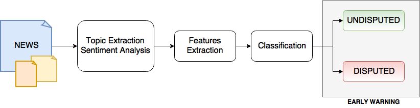
Fig. 1. Overview of the proposed framework.
content propagation cascades. Thus, to address misinformation problem properly, users’ behavior
has to be taken into account.
In this work, we introduce a general framework for a timely identification of polarizing content
on social media and, thus, the “prediction” of future fake news topics. Moreover, the output of our
framework –i.e., whether a topic is susceptible to misinformation– may be used as a new feature in
a classifier aiming at recognizing fake news. The novelty of our contribution is three-fold:
(1) To our knowledge, this is the first work dealing with the problem of the early detection of
possible topics for fake news;
(2) We introduce new features that account for how news are presented and perceived on the
social network;
(3) We provide a general framework that is easily extensible to different social media platforms.
3 A FRAMEWORK FOR THE EARLY WARNING
In this paper, we introduce a general framework to promptly determine polarizing content and
detect potential breeding ground (early warning) of either hoaxes, or fake, or unsubstantiated news.
The proposed approach is suitable to different social media platforms –e.g., Facebook, Twitter– and
consists in four main phases, as shown in Figure 1:
1. Data collection: First, we identify two categories of news sources: 1) official, and 2) fake
–i.e., aiming at disseminating unsubstantiated or fake information. Then, for each category,
we collect all data available on the platform under analysis.
2. Topic extraction and sentiment analysis: Second, we extract the topics (entities) and sen-
timent associated to our data textual content. Entity extraction adds semantic knowledge to
content to help understand the subject and context of the text that is being analyzed, allowing
to identify items such as persons, places, and organizations that are present in the input text.
3. Features definition: We now use the information collected in the previous steps to derive
a series of features that take into account how information is presented and perceived on the
platform.
4. Classification: Finally, we perform the classification task using different state-of-the-art
machine learning algorithms and comparing their results. Once detected the best algorithms
(and the related feature sets), we are ready to classify entities and, thus, identify potential
targets for fake news.
3.1 Features
For the sake of simplicity, in the following we define our features for Facebook. However, the
adaptation of the same features to other social media (e.g., Twitter, Instagram, YouTube) is straight-
forward. Let e be an entity –i.e., one of the main items/topics in a Facebook post. We say a user to:4 M. Del Vicario et al.
be engaged in entity e if she/he left more than 95% of her/his comments on posts containing e 1 . We
define the following features:
(1) The presentation distance dp (e) i.e., the absolute difference between the maximum and the
minimum value of the sentiment score of all posts containing entity e;
(2) The mean response distance dr (e) i.e., the absolute difference between the mean sentiment score
on the posts containing the entity and the mean sentiment score on the related comments;2
(3) The controversy of the entity C(e):
(
0, if dp (e) < δp
C(e) =
1, if dp (e) ≥ δp
where δp is a specific threshold dependent on the data;
(4) The perception of the entity P(e) as:
(
0, if dr (e) < δr
P(e) =
1, if dr (e) ≥ δr
where δr is a specific threshold dependent on the data;
(5) The captivation of the entity κ(e):
(
0, if ue < ρ e
κ(e) = ρ e ∈ [0, 1]
1, if ue ≥ ρ e
where ue is the fraction of users engaged in entity e and ρ e is a threshold dependent on the
data.
Let E be the set of all entities and D the (number of) entities appearing in both categories –official
and fake– of news sources (hereafter referred as disputed entities). To select the thresholds δp , δr ,
and ρ e , for each considered feature C(e), P(e), and κ(e), respectively, we define the following pairs:
• (Eδp , D δp ), where Eδp (respectively, D δp ) is the number of all (respectively, disputed) entities
in E for which dp (e) ≥ δp ;
• (Eδr , D δr ), where Eδr (respectively, D δr ) is the number of all (respectively, disputed) entities
in E for which dr (e) ≥ δr ;
• (E ρ e , D ρ e ), where E ρ e (respectively, D ρ e ) is the number of all (respectively, disputed) entities
in E for which ue ≥ ρ e .
A coherent and deep analysis of such metrics allows to determine the thresholds δp , δr , and
ρ e , that are clearly dependent on the data –and, thus, on the specific platform under analysis. In
Section 4 we exhaustively discuss a real use-case of our framework on Facebook. However, the
adaptation to similar platforms is straightforward.
3.2 Classification
To identify topics that are potential targets for fake news, we compare the performance of several
state-of-the-art classification algorithms, thus select the best ones and extract a set of features
capable of ensuring a noteworthy level of accuracy. To this aim, we rely on the Python scikit-Learn
package [28] and, on the basis of the most recent literature [29–36], we consider the following
classifiers: Linear Regression (LIN) [37], Logistic Regression (LOG) [38], Support Vector Machine
(SVM) [39] through support vector classification, K-Nearest Neighbors (KNN) [40], and Neural
Network Models (NN) [41] through the Multi-layer Perceptron L-BFGS algorithm, and Decision
1 Notice that a user may be engaged with more than one entity.
2 We also consider minimum, maximum, and the standard deviation for this measure.Polarization and Fake News: Early Warning of Potential Misinformation Targets :5
Trees (DT) [42]. To validate the results, we split the data into training (60%) and test sets (40%) and
make use of the following metrics:
• Accuracy, that is the fraction of correctly classified examples (both true positives Tp and true
negatives Tn ) among the total number of cases (N) examined:
Tp + Tn
Accuracy =
N
• Precision, that is the fraction of true positives (Tp ) over the number of true positives plus the
number of false positives (Fp ):
Tp
Precision =
Tp + Fp
• Recall, that is the fraction of true positives (Tp ) over the number of true positives plus the
number of false negatives (Fn ):
Tp
Recall =
Tp + Fn
• F1 -score, that is the harmonic mean of Precision and Recall [43]:
Precision · Recall
F 1 -score = 2 ·
Precision + Recall
• Finally, the False Positive (FP) Rate (or Inverse Recall), that is the fraction of false positives
(Fp ) over the number of false positives plus the number of true negatives (Tn ):
Fp
FP Rate =
Fp + Tn
To evaluate and compare the classifiers output we measure the accuracy of the predicted values
through the Area Under the ROC Curve (AUC), where the Receiver Operating Characteristic (ROC) is
the curve that plots the Recall against the FP Rate at various thresholds settings [44].
4 A REAL USE-CASE: FACEBOOK
In this section, we describe a real use-case of the proposed framework on Facebook. Our final aim
is to identify the topics that are most likely to become a target for future fake news.
4.1 Data collection
We identify two main categories of Facebook pages associated to:
(1) Italian official newspapers (official);
(2) Italian websites that disseminate either hoaxes or unsubstantiated information or fake news
(fake).
To produce our dataset, for set (1) we followed for the exhaustive list provided by ADS3 [45], while
for set (2) we relied on the lists provided by very active Italian debunking sites [46, 47]. To validate
the list, all pages have then been manually checked by looking at their self-description and the
type of promoted content. For each page, we downloaded all the posts in the period 31.07–12.12
2016, as well as all the related likes and comments. The exact breakdown of the dataset is provided
in Table 1. The entire data collection process was performed exclusively by means of the Facebook
Graph API [48], which is publicly available and can be used through one’s personal Facebook user
account. We used only public available data (users with privacy restrictions are not included in
3 ADS is an association for the verification of newspaper circulation in Italy. Their website provides an exhaustive list of
Italian newspaper supplying documentation of their geographical and periodical diffusion.:6 M. Del Vicario et al.
Table 1. Breakdown of the dataset (Facebook).
Official Fake
Pages 58 17
Posts 333, 547 51, 535
Likes 74, 822, 459 1, 568, 379
Comments 10, 160, 830 505, 821
Shares 31, 060, 302 2, 730, 476
our dataset). Data was downloaded from Facebook pages that are public entities. When allowed
by users’ privacy specifications, we accessed public personal information. However, in our study
we used fully anonymized and aggregated data. We abided by the terms, conditions, and privacy
policies of Facebook.
4.2 Topic extraction and sentiment analysis
To perform topic extraction and sentiment analysis, we rely on Dandelion API [49], that is partic-
ularly suited for the Italian language and gets good performances on short texts as well [50]. By
means of the Dandelion API service, we extract the main entities and the sentiment score associated
to each post of our dataset, whether it has a textual description or a link to an external document.
Entities represent the main items in the text that, according to the service specifications, could fall
in one of six categories: person, works, organizations, places, events, or concepts. Thus, for each
post we get a list of entities and their related confidence level, and a sentiment score ranging from
−1.0 (totally negative) to 1.0 (absolutely positive). During the analysis, we only considered entities
with a confidence level greater than or equal to 0.6, hereafter referred as sample E 1 . Moreover, we
selected all entities with a confidence level greater than or equal to 0.9 and occurring in at least
100 posts. For these entities, hereafter referred as sample E 2 , we selected all the posts where they
appeared and run Dandelion API to extract the sentiment score of the related comments. Details of
both samples are shown in Table 2.
Table 2. Entities Samples.
E1 E2
Official Fake Official Fake
Entities 82, 589 19, 651 1, 170 763
Posts 121, 833 5, 995 16, 098 8, 234
Comments 6, 022, 299 135, 988 1, 241, 703 171, 062
4.3 Features
Following the features presented in Section 3.1, it is straightforward to compute the presentation
distance dp (e) and the mean response distance dr (e) for each entity of our samples E 1 and E 2 . To
calculate controversy, perception and captivation, we first need to find proper thresholds for our
data. To develop an intuition on how to determine such quantities, let us analyze the behavior
of the number of disputed entities as a function of the thresholds. In Figure 2 we show for both
samples E 1 (left) and E 2 (right) the number of disputed entities D δp with presentation distance ≥ δp
normalized with respect to the total number of disputed entities D. We observe that D δp /D presents
a plateau between two regions of monotonic decrease with respect to δp . This behavior indicatesPolarization and Fake News: Early Warning of Potential Misinformation Targets :7
E1 : D δp /Eδp D δp /D E2 : D δp /Eδp D δp /D
1 1
0.8 0.8
0.6 0.6
0.4 0.4
0.2 0.2
0 0
0 0.5 1 1.5 2 0 0.5 1 1.5 2
δp (e) δp (e)
(a) (b)
Fig. 2. We show in dashed blue D δp /D, the fraction of disputed entities with presentation distance greater than
or equal to δp , and in solid orange D δp /Eδp , the ratio of disputed entities w.r.t. all entities with presentation
distance greater than or equal to δp , both for sample E1 (a) and E2 (b). The plateaus in the curves indicate
that entities are well separated into a set on uncontroversial (low δp ) and a set of controversial entities (high
δp ).
that entities are clearly separated in two sets and that all the entities with dp (e) ≥ δp are indeed
controversial. Consequently, we may take the inflection point corresponding to the second change
in the curve concavity as our threshold δp (e), since it accounts for the majority of disputed entities.
To do that, we fit our data to polynomial functions and compute all inflection points. We get the
following thresholds for C(e): δp (e) = 1.1 for sample E 1 and δp (e) = 0.98 for sample E 2 . Notice that
the height of the plateau corresponds to the size of controversial news (i.e. dp (e) > δp ): hence, for
E 1 and E 2 we have that respectively ∼ 55% and ∼ 40% of the disputed entities are controversial.
In Figure 2 we show the ratio D δp /Eδp , that measures the correlation between disputed entities D
and all entities E by varying presentation distances. Notice that the fact that D δp /Eδp → 1 when δp
grows indicates that the all highly controversial entities are also disputed entities. Like D δp /D, also
D δp /Eδp shows a plateau in the same region of δp ’s. We observe that the main difference between
the two samples E 1 and E 2 is in the initial value of D δp /Eδp and the height of the plateaus. For
sample E 2 , the total number D δp =0 of disputed entities is about ∼ 60% of the total number of entities
Eδp =0 , while for E 1 it is only ∼ 20%. On the same footing, we have that the different height of the
plateaus indicates that while for set E 1 45% of controversial news are also disputed (i.e. they belong
both to the official and fake categories), for set E2 this ratio becomes ∼ 80%
An analogous approach may be used to find the thresholds δr and ρ e for features perception
P(e) and captivation κ(e), respectively. Notice that such features are only applicable to sample E 2 ,
for which the sentiment score is available for comments too.
In Figure 3 (a) we show the fraction D δr /D of disputed entities with response distance dr greater
than or equal to δr and the ratio D δr /Eδr among disputed entities with dr ≥ δr and entities with
the same dr ≥ δr . By definition, D δr /D is a decreasing function of δr but this time it is not present
an evident plateau indicating a clearcut division into two distinct subsets. Also, unlike Figure 2,
the quantity D δr /Eδr is monotonically decreasing. Such a behavior indicates that the higher the:8 M. Del Vicario et al.
presentation distance, the lower the probability that such post is disputed, i.e. there is a higher
probability to have disputed entities – and hence a higher probability of dealing with fake news –
when the users’ response is consonant with the presentation given by news sources. The quantity
D δr /Eδr starts from an initial value of ∼ 0.6 that is followed by a sudden downfall.
In Figure 3 (b) we show the fraction D ρ e /D of disputed entities engaging a fraction of users ≥ ρ e
and the ratio D ρ e /E ρ e among disputed entities and entities engaging a fraction of users ≥ ρ e . We
observe that again D ρ e /D does not show a clearcut plateau. The same lack of a plateau happens for
D ρ e /E ρ e , that this time is an increasing quantity. Such result indicates that the higher the share of
engaged users, the higher the probability that a post is debated. In particular, we can read from the
curve (ρ e → 1) that ∼ 90% of the most viral posts is disputed.
Notice that since we observe a monotonic behavior, the inflection point is just a proxy of the
separation point among two subsets fo entities with high and low values of the analyzed threshold
parameter. By fitting our data to polynomial functions and computing all inflection points, we get
the thresholds δr (e) = 0.27 and ρ e = 0.42.
E2 : D δr /Eδr D δr /D E2 : D ρ e /E ρ e D ρ e /D
1 1
0.8
0.8
0.6
0.6
0.4
0.4
0.2
0.2
0
0 0.5 1 1.5 2 0 0.2 0.4 0.6 0.8 1
δr (e) ρe
(a) (b)
Fig. 3. Panel (a): D δr /D (dashed blue) and D δr /Eδr (solid yellow). The monotonic decrease of the ratio among
disputed entities and entities with response distance ≥ δr indicates that disputed entities do not generate
much debates and critics from their audience. Panel (b): D ρ e /D (dashed blue) and D ρ e /E ρ e (solid green). The
monotonic increase of the ratio among disputed entities and entities with user share ≥ ρ e indicates that
most viral posts can reach up to ∼ 90% of the basin of possible users.
4.4 Classification
Now that we have defined all the features, we are ready for the last step of our framework i.e., the
classification task. Our aim is to identify entities that are potential targets for fake news. In other
words, we want to assess if an entity, and hence a topic, found on a post has a high probability
to be soon found on fake news as well. Table 3 provides a list of all the features employed in our
classifiers. Notice that the main difference consists in the fact that sample E 2 also benefits from
features involving the sentiment score of users comments (features 6–11).
As illustrated in Section 3.2, we compare the results of different classifiers: Linear Regression
(LIN), Logistic Regression (LOG), Support Vector Machine (SVM) with linear kernel, K-NearestPolarization and Fake News: Early Warning of Potential Misinformation Targets :9
Table 3. Early Warning. Features.
ID Feature name N. of features Sample
1 Occurrences 1 E1, E2
2 Min/Max/Mean/Std sentiment score on posts 4 E1, E2
3 Presentation distance 1 E1, E2
4 Number of negative posts 1 E1, E2
5 Controversy 1 E1, E2
6 Min/Max/Mean/Std sentiment score on comments 4 E2
7 Min/Max/Mean/Std response distance 4 E2
8 Comments count 1 E2
9 Number of negative comments 1 E2
10 Perception 1 E2
11 Captivation 1 E2
Table 4. Early Warning: Classification Results. We report the performances for the four best performing
algorithms (LOG, SVM, KNN, NN). The first reported value refers to E 2 , while that for E 1 is in parenthesis.
Values in bold denote the two best algorithms. W. Avg. denotes the weighted average across the two classes.
AUC Accuracy M. Abs. Err. Precision Recall FP Rate F1-score
Undisputed 0.74(0.77) 0.95(0.92) 0.50(0.42) 0.83(0.84)
LOG 0.73 (0.76) 0.77 (0.79) 0.23 (0.21) Disputed 0.87(0.84) 0.50(0.59) 0.05(0.08) 0.63(0.69)
W. Avg. 0.79(0.80) 0.77(0.79) 0.28(0.25) 0.75(0.78)
Undisputed 0.75(0.81) 0.77(0.89) 0.38(0.32) 0.76(0.85)
SVM 0.68 (0.74) 0.71(0.80) 0.29(0.20) Disputed 0.64(0.80) 0.62(0.67) 0.32(0.11) 0.63(0.73)
W. Avg. 0.71(0.80) 0.71(0.80) 0.35(0.21) 0.71(0.80)
Undisputed 0.71(0.80) 0.77(0.84) 0.58(0.31) 0.74(0.82)
KNN 0.60 (0.75) 0.67(0.78) 0.33(0.22) Disputed 0.60(0.74) 0.53(0.69) 0.23(0.16) 0.56(0.71)
W. Avg. 0.66(0.78) 0.67(0.78) 0.35(0.23) 0.67(0.78)
Undisputed 0.71(0.79) 0.92(0.92) 0.57(0.37) 0.80(0.85)
NN 0.68 (0.77) 0.72 (0.80) 0.28 (0.20) Disputed 0.77(0.84) 0.42(0.63) 0.08(0.08) 0.55(0.72)
W. Avg. 0.73(0.81) 0.72(0.80) 0.32(0.22) 0.70(0.80)
Neighbors (KNN) with K = 5, Neural Network Models (NN) through the Multi-layer Perceptron
L-BFGS algorithm, and Decision Trees (DT) with Gini Index. Given the asymmetry of our dataset
in favor of official news sources, we re-sample the data at each step in order to get two balanced
groups. For the sake of simplicity, in Table 4 we report the classification results only for the four
best performing algorithms. We may notice an appreciable high accuracy –especially for the case of
data sample E 1 – and observe that all algorithms are able to accurately recognize undisputed topics,
however their ability decreases in the case of disputed ones. Moreover, we notice a significantly
low FP Rate for the case of disputed entities achieved by both LOG and NN, meaning that even
though they are more difficult to detect, there is also a smaller probability to falsely label a disputed
entity as not.
Once detected the two best algorithms –i.e., LOG and NN– we use them to classify entities again.
Specifically, we take the whole samples –E 1 and E 2 – and we make predictions about the potentiality
of each entity to become object of fake news by using either LOG or NN. We then keep the two
predicted values for each entity. Looking at the AUC score, we may determine the best performing
features for our classifier. We use the forward stepwise features selection where, starting from an:10 M. Del Vicario et al.
Table 5. Early Warning. Best performing features.
LOG NN
E1 E2 E1 E2
1 Presentation distance Occurrences Presentation distance Presentation distance
2 Captivation Std response distance Captivation Occurrences
3 Mean post sent. score Min response distance Min post sent. score Captivation
4 Controversy Std comm. sent. score Max post sent. score Mean comm. sent. score
5 Min post sent. score Min comm. sent. score Std post sent. score Mean response distance
6 Max post sent. score Captivation Number negative posts Perception
7 Number negative posts Mean comm. sent. score Controversy Max response distance
empty set of features, we iteratively add the best performing one among the unselected, when
tested together with the best ones selected so far. Table 5 reports the best seven features, for E 1
and E 2 , for both algorithms LOG and NN. Note that the newly introduced measures (in bold) –i.e.,
presentation distance, response distance, controversy, perception, and captivation– are always
among the best performing features. Moreover, we observe that the presentation distance is the
best performing feature in all cases, with the exception of the logistic regression on E 2 , where
instead we find the response distance to be among the first three.
4.5 Insights
We observed that both presentation and response distance play a primary role in the classification
of disputed topics and are among the best features of our classifier. Thus, it is worth studying in
deep such measures to better understand users’ behavior on the platform.
Looking at Figure 4, we may observe a positive relationship between an entity’s presentation
distance and the attention received in terms of likes and comments. Indeed, entities that are
presented in a different way by official and fake news sources get on average a higher number of
likes and comments and, hence, a higher attention.
Figure 5 shows a series of violin plots representing the estimated probability density function of
the mean response distance. The measure is computed for the two classes of entities –controversial
(C) and uncontroversial (UC)– and for both disputed (D) and undisputed (UD) entities. We may
notice some significant differences: distributions of controversial entities show a main peak around
0.4, which is larger in the case of disputed entities and followed by a smaller peak around 0.6,
whereas distributions of uncontroversial entities are centered around smaller values and present
two peaks, which are of similar size in the case of disputed entities. This evidence suggests that
for controversial entities users’ response is usually divergent (mean response distance near to 0.4)
from the post presentation, while for uncontroversial ones there are mixed responses, that can be
either similar to the presentation (mean response distance near to 0) or slightly divergent (mean
response distance near to 0.25). Also, it may indicate that there is a higher probability of divergent
response for disputed entities.
Finally, Figure 6 shows the Frequency of the temporal distance between the first appearance of
an entity in official information and the consequent first appearance in a fake news. Data refer to
the following categories of entities: all (ALL), controversial (C), arousing controversial response
(R), captivating (P). We may observe that the emergence of an entity on fake news is confined to
about 24 hours after its first appearance into official news. Moreover, it is worth noting that out of
about 2K unique entities appearing on official newspapers, about 50% is also the subject of either a
hoax or fake news, and the same percentage of entities shows up on fake news only after a first
apparison on official news.Polarization and Fake News: Early Warning of Potential Misinformation Targets :11
Likes Comments
104
103
102
0 0.5 1 1.5 2
δp
Fig. 4. Mean number of likes (solid purple) and comments (dashed green) for entities whose presentation
distance dp (e) ≥ δp .
1.5
C
UC
Mean response distance
1
0.5
0
D UD
Fig. 5. Estimated probability density function of the mean response distance for controversial (C) (dotted
violet) and uncontroversial (UC) (aquamarine) entities by disputed (D) and undisputed (UD) entities.
5 CAN WE DETECT FAKE NEWS?
As we have seen, we are now able to issue a warning about topics that require special caution. This
could be a crucial element of a broader system aiming at monitoring information flow constantly
and in real time. As a further step, we want to exploit the output of our framework –i.e., whether a
topic would appear in fake news or not– to build a new feature set for a classification task with
the aim of distinguishing fake news from reliable information. To this end, we show a possible:12 M. Del Vicario et al.
ALL C P R
0.35
0.3
0.25
frequency
0.2
0.15
0.1
0.05
0
1 5 10 15 20 24
hours
Fig. 6. Frequency of the temporal distance between the first appearance of an entity and the consequent first
appearance of an hoax containing that entity, for the following classes of entities: all (ALL), controversial (C),
arousing controversial response (R), and captivating (P).
application to Facebook data. As always, the approach is easily reproducible and suitable to other
social media platforms.
5.1 Instantiation to Italian News on Facebook
Let us consider two samples, P1 and P2 , that are built from E 1 and E 2 (see Section 4.2) by taking all
the news –i.e. the posts– containing such entities. More specifically, let P be the set of all posts
in our dataset. We define: Pi = {p ∈ P : ∃e ∈ Ep |e ∈ Ei } for i ∈ {1, 2} where Ep represents the
set of all entities contained in post p. As before, the main difference between the samples is the
availability of sentiment scores for comments in the second one.
We apply our framework for the early warning to each sample E 1 and E 2 , and consider their
respective parameters and best classifiers, obtaining two separate sets of new features. In specifying
such features, we account for the total number of predicted disputed entities and their rate, getting
a total of four features, two for any of the two adopted algorithms. Under this perspective, the
particularly low FP Rate of disputed entities results to be especially suited to our aim. Indeed, we
may retain less information, but with a higher level of certainty. As shown in Section 4.4, to assess
the potentiality of a topic to become object of fake news, our framework provides two predicted
values for each entity, one for each classifier –LOG and NN. We now use these values to build two
new features, that will be used in a new classifier –along with other features– with the aim of
detecting fake news. Specifically, we may define five categories of features:
(1) Structural features i.e., related to news structure and diffusion;
(2) Semantic features i.e., related to the textual contents of the news;
(3) User-based features i.e., related to users’ characteristics in terms of engagement and polariza-
tion;
(4) Sentiment-based features, which refer to both the way in which news are presented and
perceived by users;Polarization and Fake News: Early Warning of Potential Misinformation Targets :13 (5) Predicted features, obtained from our framework. The complete list of features used for both samples is reported in Table 6. To assess the relevance and the full predictive extent of each features category, we perform two separate five-step experiments. In the first one, experiment A, we test the performance of the introduced state-of-the-art binary classifiers by first considering structural features alone and then adding only one of the features’ category at each subsequent step, for both samples P 1 and P2 . While in experiment B we consider again only structural features in the first step and then we sequentially add one of the features’ category at each step. Hence for each algorithm and each experiment we get ten different trained classifiers, five for P 1 and five for P2 , where the considered categories for experiment A are: 1) structural (ST), 2) structural and semantic (ST+S), 3) structural and user-based (ST+UB), 4) structural and sentiment-based (ST+SB), 5) structural and predicted features (ST+P); while for experiment B they are: 1) structural (ST), 2) structural and semantic (ST+S), 3) structural, semantic, and user-based (ST+S+UB), 4) structural, semantic, user-based, and sentiment-based (ST+S+UB+SB), 5) structural, semantic, user-based, sentiment-based, and predicted features (ST+S+UB+SB+P). Again, we apply different classifiers: Linear Regression (LIN), Logistic Regression (LOG), Support Vector Machine (SVM) with linear kernel, K-Nearest Neighbors (KNN) with K = 5, Neural Network Models (NN) through the Multi-layer Perceptron L-BFGS algorithm, and Decision Trees (DT) with Gini Index. Given the asymmetry of our dataset in favor of official news sources, we re-sample the data at each step in order to get two balanced groups. We compare the results by measuring the accuracy of the predicted values through the AUC score. In Figure 7 we report the AUC values for the two five-steps experiments. We only focus on the results of the four best performing algorithms i.e., LIN, LOG, KNN, and DT. Experiment A, shows that semantic features are the ones bringing the highest improvement w.r.t. the baseline on structural features. However, we also observe remarkable improvements for the predicted features, regardless of their small number. When looking at experiment B, we observe a significant increment in the AUC during the last step (ST+S+UB+SB+P) with respect to previous ones4 , and this is especially evident for logistic regression and decision trees on P 2 . Moreover, from Figure 7, we can see that logistic regression is the best performing algorithm and that it achieves especially high results on P 2 . We should also notice the relative predictive power of structural features, as a matter of fact the introduction of semantic features brings, in all cases, the largest jump in the accuracy. Table 7 reports classification results for the four top-ranked classifiers –LIN, LOG, KNN, and DT– on our two samples P1 and P2 , considering all defined features categories. We notice an overall very high level of accuracy, where the best score is 0.91 and it is achieved by logistic regression on P2 , with respective precision rates in the detection of fake and not fake equal to 0.88 and 0.94. Our classifiers are generally more accurate in the detection of not fake information, however both false positive rates for fake and not fake are significantly low (especially in the LOG case), with a slightly smaller probability of falsely labeling a not fake as fake. 4 The only exceptions are for k-nearest neighbors on P 1 , where we observe the highest accuracy on step 2, and for decision trees on P 1 , where instead we observe a decrement in the accuracy in the last step.
:14                                                                                              M. Del Vicario et al.

  Table 6. Features adopted in the classification task. We count a total of 52 features for sample
  P2 and 44 for sample P1 .

      Class              Feature name                                   Posts   Comments   N. of features Sample
                         Number of likes/comments/shares           x            -          3             P1 , P2
      STRUCTURAL         Number of likes/comments on comments      -            x          2             P1 , P2
                         Average likes/comments on comments        -            x          2             P1 , P2
                         Number of characters                      x            x          2             P1 , P2
                         Number of words                           x            x          2             P1 , P2
                         Number of sentences                       x            x          2             P1 , P2
      SEMANTIC           Number of capital letters                 x            x          2             P1 , P2
                         Number of punctuation signs               x            x          2             P1 , P2
                         Average word lengtha                      x            x          2             P1 , P2
                         Average sentence length a                 x            x          2             P1 , P2
                         Punctuation rateb                         x            x          2             P1 , P2
                         Capital letters rateb                     x            x          2             P1 , P2
                         Av./Std comments to commenters            -            -          2             P1 , P2
                         Av./Std likes to commenters               -            -          2             P1 , P2
                         Mean std likes/comments to commenters     -            -          2             P1 , P2
      USER-BASED         Av./Std comments per user                 -            -          2             P1 , P2
                         Av./Std pages per user                    -            -          2             P1 , P2
                         Total engaged usersc                      -            -          1             P1 , P2
                         Rate of engaged users c                   -            -          1             P1 , P2
                         Sentiment score                           x            -          1             P1 , P2
                         Av./Std comments’ sentiment score         -            x          2             P2
                         Rate positive/negative comments           -            -          2             P2
      SENTIMENT-BASED    Number of positive over negative comments x            -          1             P2
                         Mean/Std presentation distance            x            -          2             P1 , P2
                         Number/Rate of captivating entitiesd      x            -          2             P2
                         Av. response distance                     -            -          1             P2
                                                   e
                         Numb. of pred. D entities (LOG, NN)       -            -          2             P1 , P2
      PREDICTED          Rate of pred. D entitiese (LOG, NN)       -            -          2             P1 , P2

  a Average length computed w.r.t. both posts and comments.
  b Over total number of characters.
  c Users engaged with any of the entities detected in the post.
  d Entities for which κ(e) = 1 (see Section 3.1 for details).
  e Our framework for the early warning allows to classify an entity as disputed or not. Here we consider disputed

  entities predicted through logistic regression (LOG) and neural networks (NN), since they proved to be the best
  performing algorithms (see Section 4.4 for details).

   We select the best performing features on the basis of their AUC score, employing the forward
stepwise features selection (see Section 4.4). In Table 8 we report the 16 best performing features
for both samples P1 and P2 . We note that predicted features are among the best performing features
in both cases, however structural and semantic features are the most represented. Also, the mean
presentation distance appears among the best in both columns. We may deduce that the newly
introduced sentiment-base and predicted features are extremely relevant for the purpose of fake
news identification. Moreover, the potential influential character of the commenters, embodied
in the average number of comments to the commenters, is either the first or the second best
performing features, underling the, often neglected, primary role of intermediate nodes in the
diffusion of fake news.
Polarization and Fake News: Early Warning of Potential Misinformation Targets :15
ST ST+S ST ST+S
ST+UB ST+SB ST+UB ST+SB
ST+P ST+P
0.95 0.95
0.9 0.9
0.85 0.85
P1
P2
0.8 0.8
0.75 0.75
0.7 0.7
LIN
LOG
KNN
DT
LIN
LOG
KNN
DT
(a) (b)
ST ST+S ST ST+S
ST+S+UB ST+S+UB+SB ST+S+UB ST+S+UB+SB
ST+S+UB+SB+P ST+S+UB+SB+P
0.95 0.95
0.9 0.9
0.85 0.85
P1
P2
0.8 0.8
0.75 0.75
0.7 0.7
LIN
LOG
KNN
DT
LIN
LOG
KNN
DT
(c) (d)
Fig. 7. AUC values for experiment A on (a) P1 and (b) P2 and experiment B on (c) P 1 and (d) P2 for the
following categories of features: structural (ST), semantic (S), user-based (UB), sentiment-based (SB), and
predicted (P).
6 CONCLUSIONS
In this article, we presented a general framework for a timely identification of polarizing content
that enables to 1) “predict” future fake news topics on social media, and 2) build a classifier for
fake news detection. We validated the performances of our methodology on a massive dataset of
official news and hoaxes on Facebook, however an extension to other social media platforms is
straightforward. Our analysis shows that a deep understanding of users’ behavior and polarization
is crucial when dealing with the problem of misinformation. To our knowledge, this is the first
attempt towards the early detection of possible future topics for fake news, still not without
limitations –mainly due to the fact that fake or unsubstantiated information is often diffused even:16 M. Del Vicario et al.
Table 7. Classification results. We report the performances for the 4 best performing algorithm (LIN, LOG,
KNN, DT). The first reported values refer to P2 , as in that case we have more features for the classification
and we also get better results, while those for P 1 are in parentheses. W. Avg. denotes the weighted average
across the two classes.
AUC Accuracy M. Abs. Err. Precision Recall FP Rate F1-score
Not Fake 0.91(0.85) 0.90(0.84) 0.11(0.15) 0.91(0.85)
LIN 0.90 (0.87) 0.90(0.84) 0.10(0.16) Fake 0.88(0.84) 0.90(0.85) 0.10(0.16) 0.89(0.84)
W. Avg. 0.90(0.84) 0.90(0.84) 0.11(0.16) 0.90(0.84)
Not Fake 0.94(0.90) 0.90(0.87) 0.07(0.10) 0.92(0.88)
LOG 0.94 (0.89) 0.91 (0.88) 0.09 (0.12) Fake 0.88(0.87) 0.93(0.90) 0.10(0.13) 0.90(0.88)
W. Avg. 0.91(0.88) 0.91(0.88) 0.08(0.12) 0.91(0.88)
Not Fake 0.90(0.82) 0.86(0.82) 0.11(0.18) 0.88(0.82)
KNN 0.89 (0.86) 0.87(0.82) 0.13(0.18) Fake 0.84(0.81) 0.89(0.82) 0.14(0.18) 0.87(0.82)
W. Avg. 0.87(0.82) 0.87(0.82) 0.13(0.18) 0.87(0.82)
Not Fake 0.92(0.86) 0.86(0.83) 0.09(0.14) 0.89(0.84)
DT 0.90 (0.83) 0.89(0.85) 0.11(0.15) Fake 0.85(0.83) 0.91(0.86) 0.14(0.17) 0.88(0.85)
W. Avg. 0.89(0.85) 0.89(0.84) 0.12(0.16) 0.89(0.84)
Table 8. Best performing features for post classification. Labels P and C indicate if the feature is com-
puted w.r.t. either posts or comments. For each sample we report the feature and its respective category.
P1 P2
Feature Cat. Feature Cat.
1 Av. numb. of comments to comm.ers UB Number of words (P) S
2 Numb. of predicted entities disputed (NN) P Av. numb. of comments to comm.ers UB
3 Number of words (P) S Number of likes (P) ST
4 Number of likes (P) ST Number of shares (P) ST
5 Number of shares (P) ST Capital letters rate (P) S
6 Std numb. of likes to comm.ers UB Number of comments (C) ST
7 Number of capital letters (P) S Number of comments (P) ST
8 Number of punctuation signs (P) S Av. comments per user UB
9 Std numb. of comments per user UB Number of sentences S
10 Std sentiment score (C) SB Number of punctuation signs S
11 Number of characters (CP) S Numb. of predicted disputed entities (NN) P
12 Av. sentence length (P) S Mean presentation distance SB
13 Mean presentation distance SB Av. numb. of comments to comm. ST
14 Number of comments (C) ST Rate of polarized users UB
15 Rate of predicted disputed entities (LOG) P Std presentation distance SB
16 Rate of predicted disputed entities (NN) P Av. pages per user UB
by official newspapers. When dealing with a complex issue such as massive digital misinformation,
special caution is required. However, our results are promising and bode well for a system enabled
for monitoring information flow in real time and issuing a warning about delicate topics. In this
direction, our approach could represent a pivotal step towards the smoothing of polarization on
online social media.Polarization and Fake News: Early Warning of Potential Misinformation Targets :17
REFERENCES
[1] Statista, “Number of monthly active facebook users worldwide as of 3rd quarter 2017 (in millions),” Website, 2018. [On-
line]. Available: https://www.statista.com/statistics/264810/number-of-monthly-active-facebook-users-worldwide/
[2] O. Dictionaries, “Oxford dictionaries word of the year 2016 is...post-truth,” Website, 2017. [Online]. Available:
https://www.oxforddictionaries.com/press/news/2016/12/11/WOTY-16
[3] R. Allen, “What happens online in 60 seconds?” Website, 2017. [Online]. Available: https://www.smartinsights.com/
internet-marketing-statistics/happens-online-60-seconds/
[4] N. Newman, R. Fletcher, A. Kalogeropoulos, D. A. Levy, and R. K. Nielsen, “Reuters institute digital news report 2017,”
2017.
[5] M. Del Vicario, A. Bessi, F. Zollo, F. Petroni, A. Scala, G. Caldarelli, H. E. Stanley, and W. Quattrociocchi, “The spreading
of misinformation online,” Proceedings of the National Academy of Sciences, vol. 113, no. 3, pp. 554–559, 2016.
[6] A. L. Schmidt, F. Zollo, M. Del Vicario, A. Bessi, A. Scala, G. Caldarelli, H. E. Stanley, and W. Quattrociocchi, “Anatomy
of news consumption on facebook,” Proceedings of the National Academy of Sciences, vol. 114, no. 12, pp. 3035–3039,
2017.
[7] M. Del Vicario, F. Zollo, G. Caldarelli, A. Scala, and W. Quattrociocchi, “Mapping social dynamics on Facebook: The
Brexit debate,” Social Networks, vol. 50, no. Supplement C, pp. 6 – 16, 2017.
[8] F. Zollo, A. Bessi, M. Del Vicario, A. Scala, G. Caldarelli, L. Shekhtman, S. Havlin, and W. Quattrociocchi, “Debunking
in a world of tribes,” PLOS ONE, vol. 12, no. 7, pp. 1–27, 07 2017.
[9] W. L. Howell, “Digital wildfires in a hyperconnected world,” World Economic Forum, Tech. Rep. Global Risks 2013,
2013.
[10] W. Quattrociocchi, A. Scala, and C. R. Sunstein, “Echo chambers on facebook,” 2016.
[11] F. Zollo and W. Quattrociocchi, “Misinformation spreading on facebook,” arXiv preprint arXiv:1706.09494, 2017.
[12] S. Antoniadis, I. Litou, and V. Kalogeraki, “A model for identifying misinformation in online social networks,” in On
the Move to Meaningful Internet Systems: OTM 2015 Conferences, C. Debruyne, H. Panetto, R. Meersman, T. Dillon,
G. Weichhart, Y. An, and C. A. Ardagna, Eds. Cham: Springer International Publishing, 2015, pp. 473–482.
[13] M. Rajdev and K. Lee, “Fake and spam messages: Detecting misinformation during natural disasters on social media,”
in Web Intelligence and Intelligent Agent Technology (WI-IAT), 2015 IEEE/WIC/ACM International Conference on, vol. 1.
IEEE, 2015, pp. 17–20.
[14] C. Boididou, S. Papadopoulos, L. Apostolidis, and Y. Kompatsiaris, “Learning to detect misleading content on twitter,”
in Proceedings of the 2017 ACM on International Conference on Multimedia Retrieval. ACM, 2017, pp. 278–286.
[15] C. Boididou, S. E. Middleton, Z. Jin, S. Papadopoulos, D.-T. Dang-Nguyen, G. Boato, and Y. Kompatsiaris, “Verifying
information with multimedia content on twitter,” Multimedia Tools and Applications, pp. 1–27, 2017.
[16] A.-M. Popescu and M. Pennacchiotti, “Detecting controversial events from twitter,” in Proceedings of the 19th ACM
international conference on Information and knowledge management. ACM, 2010, pp. 1873–1876.
[17] C. Castillo, M. Mendoza, and B. Poblete, “Information credibility on twitter,” in Proceedings of the 20th international
conference on World wide web. ACM, 2011, pp. 675–684.
[18] S. Kumar, R. West, and J. Leskovec, “Disinformation on the web: Impact, characteristics, and detection of wikipedia
hoaxes,” in Proceedings of the 25th International Conference on World Wide Web. International World Wide Web
Conferences Steering Committee, 2016, pp. 591–602.
[19] S. Siersdorfer, S. Chelaru, J. S. Pedro, I. S. Altingovde, and W. Nejdl, “Analyzing and mining comments and comment
ratings on the social web,” ACM Transactions on the Web (TWEB), vol. 8, no. 3, p. 17, 2014.
[20] S. Afroz, M. Brennan, and R. Greenstadt, “Detecting hoaxes, frauds, and deception in writing style online,” in Security
and Privacy (SP), 2012 IEEE Symposium on. IEEE, 2012, pp. 461–475.
[21] Y. Mejova, A. X. Zhang, N. Diakopoulos, and C. Castillo, “Controversy and sentiment in online news,” arXiv preprint
arXiv:1409.8152, 2014.
[22] L. A. Adamic and N. Glance, “The political blogosphere and the 2004 us election: divided they blog,” in Proceedings of
the 3rd international workshop on Link discovery. ACM, 2005, pp. 36–43.
[23] K. Garimella, G. De Francisci Morales, A. Gionis, and M. Mathioudakis, “Quantifying controversy in social media,” in
Proceedings of the Ninth ACM International Conference on Web Search and Data Mining. ACM, 2016, pp. 33–42.
[24] A. Guess, B. Nyhan, and J. Reifler, “Selective exposure to misinformation: Evidence from the consumption of fake news
during the 2016 us presidential campaign,” 2018.
[25] J. Ugander, L. Backstrom, C. Marlow, and J. Kleinberg, “Structural diversity in social contagion,” Proceedings of the
National Academy of Sciences, vol. 109, no. 16, pp. 5962–5966, 2012.
[26] P. H. C. Guerra, W. Meira Jr, C. Cardie, and R. Kleinberg, “A measure of polarization on social media networks based
on community boundaries.” in ICWSM, 2013.
[27] M. Conti, D. Lain, R. Lazzeretti, G. Lovisotto, and W. Quattrociocchi, “It’s always april fools’ day! on the difficulty of
social network misinformation classification via propagation features,” arXiv preprint arXiv:1701.04221, 2017.:18 M. Del Vicario et al.
[28] F. Pedregosa, G. Varoquaux, A. Gramfort, V. Michel, B. Thirion, O. Grisel, M. Blondel, P. Prettenhofer, R. Weiss,
V. Dubourg, J. Vanderplas, A. Passos, D. Cournapeau, M. Brucher, M. Perrot, and E. Duchesnay, “Scikit-learn: Machine
learning in Python,” Journal of Machine Learning Research, vol. 12, pp. 2825–2830, 2011.
[29] I. Alsmadi and G. K. Hoon, “Term weighting scheme for short-text classification: Twitter corpuses,” Neural Computing
and Applications, pp. 1–13, 2018.
[30] S. A. Özel, E. Saraç, S. Akdemir, and H. Aksu, “Detection of cyberbullying on social media messages in turkish,” in
International Conference on Computer Science and Engineering (UBMK). IEEE, 2017, pp. 366–370.
[31] A. Khatua and A. Khatua, “Cricket world cup 2015: Predicting user’s orientation through mix tweets on twitter
platform,” in Proceedings of the 2017 IEEE/ACM International Conference on Advances in Social Networks Analysis and
Mining 2017. ACM, 2017, pp. 948–951.
[32] D. Antonakaki, I. Polakis, E. Athanasopoulos, S. Ioannidis, and P. Fragopoulou, “Exploiting abused trending topics to
identify spam campaigns in twitter,” Social Network Analysis and Mining, vol. 6, no. 1, p. 48, 2016.
[33] J. Hemsley, S. Tanupabrungsun, and B. Semaan, “Call to retweet: Negotiated diffusion of strategic political messages,”
in Proceedings of the 8th International Conference on Social Media & Society. ACM, 2017, p. 9.
[34] W. van Zoonen and G. Toni, “Social media research: The application of supervised machine learning in organizational
communication research.” Computers in Human Behavior, vol. 63, pp. 132–141, 2016.
[35] S. Vosoughi and D. Roy, “Tweet acts: A speech act classifier for twitter.” in ICWSM, 2016, pp. 711–715.
[36] C.-C. Chang, S.-I. Chiu, and K.-W. Hsu, “Predicting political affiliation of posts on facebook,” in Proceedings of the 11th
International Conference on Ubiquitous Information Management and Communication. ACM, 2017, p. 57.
[37] R. M. Rifkin and R. A. Lippert, “Notes on regularized least squares,” 2007.
[38] M. Schmidt, N. Le Roux, and F. Bach, “Minimizing finite sums with the stochastic average gradient,” Mathematical
Programming, vol. 162, no. 1-2, pp. 83–112, 2017.
[39] C. Cortes and V. Vapnik, “Support-vector networks,” Machine learning, vol. 20, no. 3, pp. 273–297, 1995.
[40] J. L. Bentley, “Multidimensional binary search trees used for associative searching,” Communications of the ACM, vol. 18,
no. 9, pp. 509–517, 1975.
[41] D. E. Rumelhart, G. E. Hinton, R. J. Williams et al., “Learning representations by back-propagating errors,” Cognitive
modeling, vol. 5, no. 3, p. 1, 1988.
[42] L. Breiman and J. Friedman, “Ra olshen and cj stone,âĂIJ,” Classification and regression trees, 1984.
[43] M. Sokolova and G. Lapalme, “A systematic analysis of performance measures for classification tasks,” Information
Processing & Management, vol. 45, no. 4, pp. 427–437, 2009.
[44] C. E. Metz, “Basic principles of roc analysis,” in Seminars in nuclear medicine, vol. 8, no. 4. Elsevier, 1978, pp. 283–298.
[45] ADS, “Elenchi testate,” Website, 2016. [Online]. Available: http://www.adsnotizie.it/_testate.asp
[46] Bufale.net, “The black list: la lista nera del web,” Website, 2016, last checked: 27.11.2017. [Online]. Available:
http://www.adsnotizie.it/_testate.asp
[47] BUTAC, “The black list,” Website, 2016, last checked: 27.11.2017. [Online]. Available: http://www.butac.it/the-black-list/
[48] Facebook, “Using the Graph API,” Website, 8 2013, last checked: 27.11.2017. [Online]. Available: https:
//developers.facebook.com/docs/graph-api/using-graph-api/
[49] SpazioDati, “Dandelion API,” Website, 8 2017. [Online]. Available: https://dandelion.eu/docs/
[50] R. F. Canales and E. C. Murillo, “Evaluation of entity recognition algorithms in short texts,” CLEI ELECTRONIC
JOURNAL, vol. 20, no. 1, 2017.You can also read