Understanding the Gains from Wage Flexibility: The Exchange Rate Connection
←
→
Page content transcription
If your browser does not render page correctly, please read the page content below
Understanding the Gains from Wage Flexibility:
           The Exchange Rate Connection
                                      y                                     z
                        Jordi Galí              Tommaso Monacelli

                                       December 2013
                                   (…rst draft: July 2013)

                                             Abstract
         We study the gains from increased wage ‡exibility and their dependence on ex-
      change rate policy, using a small open economy model with staggered price and
      wage setting. Two results stand out: (i) the impact of wage adjustments on em-
      ployment is smaller the more the central bank seeks to stabilize the exchange rate,
      and (ii) an increase in wage ‡exibility often reduces welfare, and more likely so in
      economies under an exchange rate peg or an exchange rate-focused monetary policy.
      Our …ndings call into question the common view that wage ‡exibility is particularly
      desirable in a currency union.
         Keywords: sticky wages, nominal rigidities, New Keynesian model, stabilization
      policies, exchange rate policy, currency unions, monetary policy rules.
         JEL Classi…cation No.: E32, E52, F41

     We have bene…ted from comments by Stephanie Schmitt-Grohé and participants at seminars and
conferences at CREI-UPF, NBER Summer Institute (IFM), Bonn, Pavia, Banco de Portugal, and London
Business School. Chiara Maggi provided excellent research assistance. We thank the Fondation Banque
de France for …nancial support. Part of this work has been conducted while Monacelli was visiting the
Department of Economics at Columbia University, whose hospitality is gratefully acknowledged.
   y
     CREI, Universitat Pompeu Fabra and Barcelona GSE. E-mail: jgali@crei.cat
   z
     Università Bocconi and IGIER. E-mail: tommaso.monacelli@unibocconi.it

                                                 1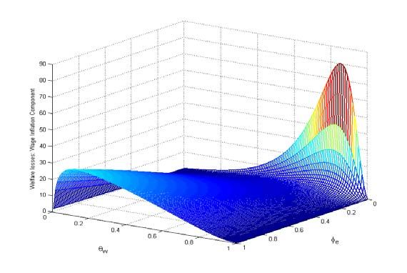
1      Introduction
The belief in the virtues of wage ‡exibility is widespread in policy circles. It manifests
itself most clearly in the recurrent calls for wage moderation (or even outright wage
cuts), issued by international policy institutions, and addressed to countries facing high
unemployment. The Great Recession and the "crisis of the euro" have only reinforced
those views.
    The case for wage ‡exibility rests on its perceived role as a factor of macroeconomic
stability. Thus, a decrease in wages is expected to o¤set, at least partly, the negative e¤ects
on employment (and output) of an adverse aggregate shock. Conversely, the presence of
rigid wages tends to amplify the employment and output e¤ects of those shocks, increasing
macroeconomic instability.1 Figure 1 illustrates that "classical" view, using a conventional
labor market diagram.
    The role of wages as a cushion is viewed as being particularly important in the context
of economies that have joined a currency union or adopted any other form of hard peg, for
in those cases the exchange rate is no longer available as an adjustment mechanism. In
the face of a country-speci…c adverse shock that calls for a real exchange rate depreciation,
a wage-based "internal devaluation" is warranted. The presence of wage rigidities, it is
argued, will hinder that adjustment, and make it longer and more painful, by requiring,
ceteris paribus, a higher rate of unemployment to bring about the needed adjustment in
wages and prices. To the extent that wage ‡exibility acts as a substitute for exchange
rate ‡exibility, it is viewed as particularly desirable in economies that have adopted a
hard peg or joined a currency union.2
    The conventional wisdom described above ignores, however, the fact that in economies
    1
      See e.g. Hall (2005) and Shimer (2005, 2012) for a discussion of the role of wage rigidities in accounting
for labor market ‡uctuations in the context of the search and matching model. Blanchard and Galí (2007,
2010) emphasize the policy tradeo¤s generated by the presence of wage rigidities.
    2
      The analysis of the interaction between wage rigidities and the exchange rate regime traces back to
Friedman (1953). Recent research on the consequences of wage rigidity in currency unions can be found
Schmitt-Grohe and Uribe (2012) and Farhi et al. (2013).

                                                       2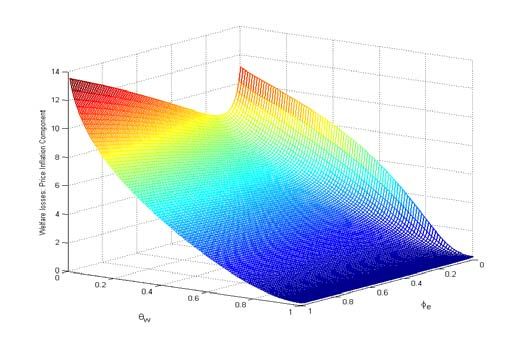
with nominal rigidities the impact of wage adjustments on employment works to a large
extent through its induced e¤ect on the endogenous component of monetary policy, as
the latter is loosened or tightened in response to lower or higher in‡ationary pressures.
We refer to this as the "endogenous policy channel.". Thus, and as argued in Galí (2013)
in the context of a closed economy model, whether an increase in wage ‡exibility raises
welfare depends on the monetary policy rule in place and, in particular, on the strength of
the central bank’s systematic response to in‡ation. If that response is weak, the bene…ts
of increased wage ‡exibility in the form of more employment stability will be small and,
in many cases, more than o¤set by the losses associated with greater volatility in price
and wage in‡ation.
   In the present paper we extend the analysis of the gains from wage ‡exibility to the
case of an open economy. As we discuss below, openness brings about two additional
factors with potentially counteracting implications. First, openness makes room for a
"competitiveness channel", whereby a reduction in domestic wages leads to a terms of
trade depreciation and, as a result, an increase in aggregate demand, output and em-
ployment. That mechanism should work to stabilize employment in the face of adverse
aggregate shocks, thus strengthening the "endogenous policy channel.". From the view-
point of the "competitiveness channel", the degree of openness of the economy and the
elasticity of net exports with respect to the real exchange rate would seem to be important
determinants of the gains from greater wage ‡exibility.
   On the other hand, monetary policy in the open economy may be driven, to a greater
or lesser extent, by the desire to stabilize the exchange rate. In the absence of capital
controls, maintaining a stable exchange rate requires that the interest rate does not deviate
much from its relevant foreign counterpart. In that case, the "endogenous policy channel"
will be dampened (or fully muted, in the case of a hard peg or a currency union), and so
will be the e¤ect of lower wages on aggregate demand and employment.
   In order to understand the role played by the exchange rate regime in determining

                                             3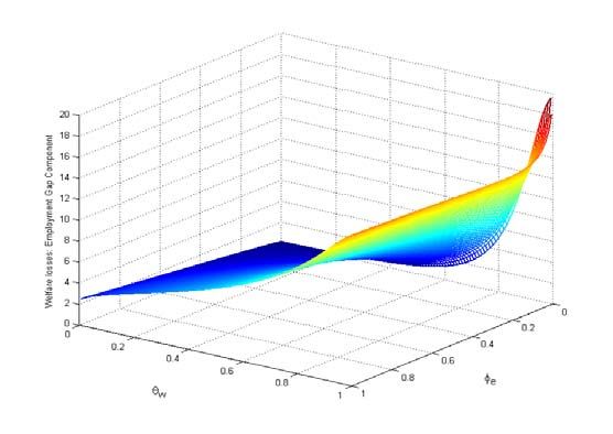
the gains from wage ‡exibility, we develop a small open economy model with staggered
price and wage setting, and study the impact of greater wage ‡exibility on macroeconomic
stability and welfare, as a function of the exchange rate policy in place. Our model builds
on the framework developed in Galí and Monacelli (2005), which we extend by allowing
for nominal wage rigidities.3
        Our analysis delivers two main …ndings. Firstly, we show that the impact of wage
adjustments on employment is smaller the more the central bank seeks to stabilize the
exchange rate. Accordingly, and contrary to conventional wisdom, wage adjustments are
particularly ine¤ective in a currency union. Secondly, an increase in wage ‡exibility often
reduces welfare, and more likely so in economies that seek to stabilize the exchange rate.
Our …ndings thus call into question the common view that wage ‡exibility is particularly
desirable in a currency union.
        The remainder of the paper is organized as follows. In Section 2 we describe our
baseline model. In Section 3 we report our main …ndings on the role of exchange rate policy
in determining the gains from increased wage ‡exibility. Section 4 analyzes the robustness
of our …ndings to departures from our baseline calibration. Section 5 discusses the related
literature. Section 6 summarizes the main lessons from the paper and concludes.

2         A New Keynesian Model of a Small Open Economy
In this section we describe the key ingredients of the model we use in our analysis of the
gains from wage ‡exibility. Our model is one of a small open economy with staggered
price and wage setting. It builds on the framework developed in Galí and Monacelli
(2005), extending the latter by introducing sticky nominal wages (in addition to sticky
prices), and a preference/demand shock (in addition to a technology shock).4 Since the
    3
    The resulting framework is similar to the one used in Campolmi (2012) and Erceg et al. (2009).
    4
    See, e.g. Campolmi (2012) and Erceg et al. (2009) for earlier examples of New Keynesian open
economies with staggered nominal wage setting.

                                                4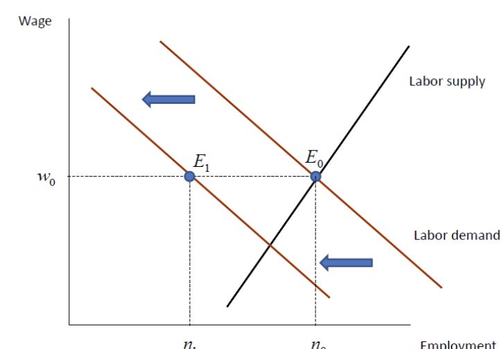
model is relatively standard, we restrict our exposition below to a description of the main
assumptions, while relegating most derivations to an Appendix.

2.1        Households

We study a small open economy inhabited by a continuum of households, indexed by
i 2 [0; 1], and with preferences given by

                                              X
                                              1
                                                     t
                                        E0               U (Ct (i); Nt (i); Xt )                                         (1)
                                              t=0

where Nt (i) denotes the amount of a di¤erentiated labor service supplied by the household,
Ct (i) is a consumption index, and Xt .is an exogenous preference shifter, common to all
domestic households. Period utility U is assumed to take the form

                                                                               1
                        U (Ct (i); Nt (i); Xt ) =         log Ct (i)              Nt (i)1+' Xt
                                                                              1+'

       Under the assumption of complete …nancial markets, and given separable utility, con-
sumption is equalized across domestic households. Thus, and in order to lighten the
notation, we henceforth drop the index i associated with household consumption.
       The consumption index is de…ned by5

                                                     1            1          1            1       1
                                  Ct     (1         ) CH;t 1          +          CF;t 1                                  (2)

with CH;t being an index of domestic goods consumption given by the CES function
                             p
         R1          p 1    p 1
CH;t      0
            CH;t (j)  p  dj     where j 2 [0; 1] denotes the good variety.6 CF;t is the
quantity consumed of a composite foreign good. Parameter                                      p   > 1 denotes the elasticity
   5
       For the limiting case of    = 1 the consumption index takes the form

                                              Ct         (CH;t )1     v
                                                                          (CF;t )v

where where       1=((1 v)(1 v) v )
  6
    As discussed below, domestic …rms produce a continuum of di¤erentiated goods, indexed by j 2 [0; 1]:

                                                              5
of substitution between varieties produced domestically. Parameter 2 [0; 1] can be
interpreted as a measure of openness.7
The (log) preference shifter, xt log Xt , is assumed to follow an exogenous AR(1)
process:
xt = x xt 1 + "xt
The period budget constraint for the typical household is given by
Z 1
PH;t (j)CH;t (j)dj + PF;t CF;t + Et fQt;t+1 Dt+1 g Dt + Wt (i)Nt (i) (3)
0
for t = 0; 1; 2; :::, where PH;t (j) is the price of domestic variety j: PF;t is the price of
the imported good, expressed in domestic currency. Dt+1 is the nominal payo¤ in period
t + 1 of the portfolio held at the end of period t (which may include shares in domestic
…rms), Wt (i) is the nominal wage for type i labor. The previous variables are all expressed
in units of domestic currency. Qt;t+1 (Ct =Ct+1 )(Pt =Pt+1 ) is the relevant stochastic
discount factor for one-period ahead nominal payo¤s.
We assume that the law of one price holds at the level of each individual variety,
implying
PF;t = Et Pt
where Et is the nominal exchange rate and Pt is the foreign price level (in foreign currency).
With little loss of generality, the latter is assumed to be constant and normalized to unity.
Each household is specialized in the provision of some di¤erentiated labor service,
for which …rms generate an isoelastic demand (see below) and for which each household
sets the corresponding nominal wage.8 Each period only a fraction 1 w of households,
drawn randomly from the population, reset their nominal wage in a way consistent with
utility maximization, subject to the demand for their labor services (current and future).
7
Equivalently, and under the assumption that the domestic economy is in…nitesimally small, 1 can
be interpreted as a measure of home bias. See Galí and Monacelli (2005) for a discussion.
8
Alternatively, one can think of many households supplying each tpe of labor, with a union representing
them setting the wage on their behalf.
6The remaining fraction w of households keep their nominal wage unchanged. Parameter
w 2 [0; 1] can be thus seen as an index of nominal wage rigidities. Much of the analysis
below explores the consequences of changes in that parameter.
As in Galí and Monacelli (2005), we assume domestic households have access to a
complete set of state-contingent securities, traded domestically and internationally.
2.2 Firms
The home economy has a continuum of domestic …rms, indexed by j 2 [0; 1]. A typical
…rm produces a di¤erentiated good using the technology
Yt (j) = At Nt (j)1
R1 w 1
w
w 1
where Yt (j) is output and Nt (j) 0
Nt (i; j) w di is a CES function of the quan-
tities of di¤erent types of labor services hired. Parameter w > 1 denotes the elasticity
of substitution between labor service varieties. At is a stochastic technology parameter,
common to all …rms. Its logarithm, at log At , follows an exogenous AR(1) process:
at = a at 1 + "at
Employment is subject to a proportional payroll tax t, common to all labor types, so
9
that the e¤ective cost of hiring one unit of type i labor service is Wt (i)(1 + t)
Each period, a subset of …rms of measure 1 p, drawn randomly, reoptimize the price
of their good, subject to a sequence of demand schedules for the latter. The remaining
fraction p keep their price unchanged. Parameter p 2 [0; 1] can thus be interpreted as
an index of price rigidities. Prices are set in domestic currency and are the same for both
the domestic and export markets. All …rms meet the demand for their respective goods
at the posted prices.
9
Note that a negative value for t should be interpreted as an employment subsidy.
72.3 Demand for Exports
We assume that the demand for domestic good j coming from the rest of the world is
given by:
p
PH;t (j)
CH;t (j) = CH;t
PH;t
R1 1
1
p
for j 2 [0; 1], where PH;t 0
PH;t (j)1 p
dj is the domestic price index. Aggregate
exports, CH;t , are in turn given by
PH;t
CH;t = Ct
PF;t
where, without loss of generality, the units in terms of which world consumption is ex-
pressed have been normalized so that in a symmetric steady state PH = PF , CH = C ;
and C = C .
For simplicity, and with little loss of generality, we assume that aggregate output and
consumption in the world economy are constant, and equal to one.
2.4 Monetary Policy
The monetary authority in the home economy is assumed to follow an interest rate rule
of the form:
e
it = + H;t + et (4)
1 e
where it is the short-term policy rate, H;t pH;t pH;t 1 denotes domestic in‡ation and
et log Et is the (log) nominal exchange rate. 1 and e 2 [0; 1] are coe¢ cients
determining the strength of the central bank’s response to deviations of in‡ation and the
(log) nominal exchange rate from their respective targets (normalized to zero).10 Note
that in the limiting case of e ! 1 we have et = 0 for all t, which corresponds to an
10
See Monacelli (2004) for an analysis of …xed exchange rates when alternative monetary policy regimes
are speci…ed according to rule (4).
8exchange rate peg.11
Throughout, and with little loss of generality, we assume that the interest rate in the
rest of the world is constant, and normalized to zero (it = 0).
2.5 Equilibrium
In the Appendix we derive the (standard) optimality conditions for the problem fac-
ing households and …rms. Combined with the market clearing conditions and after log-
linearization around the zero in‡ation steady state, they can be used to determine the set
of conditions characterizing the equilibrium of the small open economy. That equilibrium
can be represented by means of the following system of di¤erence equations (with lower
case letters denoting the natural logarithms of the original variables and with constants
ignored):
Aggregate demand block:
yt = (1 )ct + (2 )st (5)
ct = xt + (1 )st (6)
ct = Et fct+1 g (1 )(it Et f H;t+1 g) + (1 x )xt (7)
e
it = H;t + et (8)
1 e
st et pH;t (9)
1
nt = (yt at ) (10)
1
11
Alternatively, one may assume the rule:
e
it = H;t + et + et
1 e
a particular case of which, given by = , corresponds to
it = t + e et
where t pt pt 1 is CPI in‡ation.
9Aggregate supply block:
p p p
H;t = Et f H;t+1 g + yet + et
p! + p set + p t (11)
1
p
H;t pH;t pH;t 1 (12)
w w w'
t = Et f t+1 g + yet + we
ct et
w! (13)
1
w
w;t wt wt 1 (14)
!t wt (pH;t + st ) (15)
where variables with a "e" denote deviations from their natural (i.e. ‡exible price and
wage) equilibrium counterparts (e.g., yet yt ytn denotes the output gap, with ytn being
the natural level of output).
The aggregate demand block includes equation (5) determining output as a function
of aggregate demand, which in turn is expressed as a function of consumption ct and the
terms of trade st (de…ned in (9)). Consumption evolves according to Euler equation (7),
and thus responds to changes in the domestic real rate and the preference shifter.12 In
addition, domestic consumption satis…es the risk sharing condition (6).13 Equation (8)
is the interest rate rule introduced earlier. Equation (10) determines employment as a
function of aggregate output, given technology.
The aggregate supply block consists of two equations, (11) and (13), describing the
evolution of aggregate (domestic) price an wage in‡ation (de…ned, respectively, by (12)
and (14)), as a function of the output, consumption and real wage gaps (as well as the
12
Notice that the (log-linearized) consumption Euler equation features a dependence of expected con-
sumption growth on the real interest rate measured in units of domestic goods, it Et f H;t+1 g. In the
Appendix we show how this can be derived from the original Euler equation featuring the CPI-based real
interest rate, once the same condition is combined with a log-linear UIP condition and the de…nition of
CPI in‡ation.
13
The intertemporal optimality conditions of the domestic and foreign consumers can be combined to
yield, as a …rst order approximation, the interest parity condition
it = Et f et+1 g
We do not list that condition separately since it can be obtained by combining (6) and (7).
10payroll tax in the case of price in‡ation). Finally, (15) de…nes the real (consumption)
wage, as a function of the nominal wage, the domestic price and the terms of trade.14
As derived in the Appendix, natural employment, which we denote by nnt is given by
nnt = ( 1) (2 )at [1 + ( 1)(2 )]xt n t
1
where 1 +( +')[1+( 1) (2 )]
> 0. Note that under our assumptions on technology
and preferences, and in the absence of variations in the employment subsidy, natural
employment would be constant in a closed economy (i.e. under = 0). For the open
economy natural employment remains independent of technology in the special case of
= 1, but is still a¤ected by the demand shock (through the risk sharing condition).
The previous expression can be combined with other equilibrium conditions to derive
the natural values of the remaining variables. Thus, and ignoring constants,
ytn = at + (1 )nnt
snt = at xt t ( + ')nnt
cnt = xt + (1 )snt
! nt = at nnt t st
2.6 Calibration
Table 1 lists the baseline settings for the model parameters, which we use in many of the
simulations below. Most of those settings are pretty standard. The curvature of labor
disutility, ', is set to 5, a value consistent with a Frisch labor elasticity of 0:2. The
discount factor is set to 0:99. Parameter , indexing the degree of decreasing returns
to labor, is set to 0:25. Parameters p and w are set, respectively to values 4:52 and 9:
As discussed in Galí (2011), the former is consistent with a steady state unemployment
rate of 5 percent, while the latter implies a steady state price markup of 12:5 percent.
14
Note that pH;t + st = pt corresponds to the (log) CPI.
11The baseline setting for the Calvo price and wage stickiness parameters, p = w = 0:75,
implies an average duration of individual prices and wages of one year, in a way consistent
with much of the micro evidence.15 Much of the analysis below, however, examines the
consequences of variations in w, and its interaction with the exchange rate coe¢ cient
e. The in‡ation coe¢ cient in the interest rate rule is set to 1:5, the value proposed by
Taylor (1993). We set the baseline elasticity of substitution between domestic and foreign
goods, denoted by , to unity (a convenient case, as discussed below), and the openness
parameter, , to 0:4 (implying a steady state import share of 0:4). In the robustness
section we explore alternative settings for both parameters, as well as for p. Finally, we
choose 0:9 as a baseline value for persistence parameters x and a.
3 The Impact of Labor Costs on Employment: The
Role of Exchange Rate Policy
The extent to which wage ‡exibility may play a stabilizing role depends on the in‡uence
that wages (or other labor cost components) may have on employment itself. In this
section we seek to dissect the mechanism through which that in‡uence manifests itself in
our model economy.
As argued in Galí (2013), the mechanism through which adjustments in wages end up
a¤ecting employment in the New Keynesian model is very di¤erent from that in a classical
economy. In the latter, a change in the real wage directly a¤ects the quantity of labor
demanded by …rms, which is determined by the equality between the marginal product of
labor and the wage. By way of contrast, in a Keynesian environment the amount of labor
hired is determined, for a given technology, by the quantity of output that …rms want
to produce, which in turn is determined by aggregate demand. Thus, a change in wages
ends up a¤ecting employment through its (sequential) impact on marginal cost, in‡ation
and –through the policy rule–nominal and real interest rates and, hence, consumption (or
15
See, e.g., Taylor (1999), Nakamura and Steinsson (2007) and Baratieri, Basu and Gottschalk (2013).
12other interest rate-sensitive components) and aggregate demand. Thus, as demonstrated
in Galí (2013), the strength of the central bank’s response to variations in in‡ation is
a key factor in determining the response of employment to a change in wages (or other
labor costs). This is what we refer to as the "endogenous policy channel". In the open
economy, the extent to which domestic monetary policy is constrained by the desire (or
commitment) to stabilize the exchange rate, will determine the strength of the central
bank’s response to the changes in in‡ation brought about by a wage adjustment and, as
a result, the ultimate impact on employment of such an adjustment.
In order to illustrate the previous point, we simulate the response of employment to
an exogenous decline in the payroll tax, a component of the labor cost which our model
treats as exogenous.16 In a classical economy, that policy intervention would have a direct
e¤ect on labor demand and would raise employment. This is not the case in a Keynesian
environment like the one analyzed here, in which the response of employment will depend
to a great extent on how the central bank reacts to the disin‡ationary pressures triggered
by the payroll tax cut. More speci…cally, we study how the response of employment to the
payroll tax cut depends on the strength of the central bank’s response to the exchange
17
rate, as measured by e.
We assume that the payroll tax follows an exogenous AR(1) process with autoregres-
sive coe¢ cient of 0:9, and simulate the impact of a 1 percent reduction. Figure 2.a displays
the implied impulse response of employment to the payroll tax cut as a function of e.
When the central bank’s concern for exchange rate stability is weak (i.e., for values of
e close to zero) employment increases substantially in response to that policy interven-
tion. As we increase the value of e the response of employment becomes more muted.
When e is close to unity the initial impact on employment is less than a fourth of the
16
To be clear: we do not think that exogenous variations in payroll taxes or employment subsidies are
an important source of ‡uctuations in actual economies. But a change in the payroll tax provides a clean
experiment to examine the impact of changes in labor costs on employment.
17
Unless stated otherwise, the remaining parameters are set at their baseline values inall simulations.
13corresponding value for e = 0.
What explains the inverse relation between the size of the employment response and
the value of e? Equation (5) makes clear that the response of output (and, hence, of
employment, given an unchanged technology) is in turn a function of the consumption
and terms of trade responses. Next we discuss the determinants of those responses.
To understand the determinants of the consumption response, we solve equation (7)
forward to yield:
X
1
ct = x t (1 ) Et frt+k g
k=0
where rt it Et f H;t+1 g is the real interest rate, measured in terms of domestic goods.
Thus, in the absence of a preference shock, we see that the response of consumption is
inversely related to the sum of current and expected future real rates. It is easy to show
that a similar result holds for the terms of trade: by combining (6) and (7), one can derive
a "real" version of uncovered interest parity condition
st = rt + Et fst+1 g
which in turn can be solved forward to yield
X
1
st = Et frt+k g
k=0
Thus, we see that the e¤ect of a payroll tax cut on employment depends only on the
dynamic response of the real interest rate, which in the New Keynesian model is in‡uenced
by the response of monetary policy. The in‡uence of coe¢ cient e on that response is
con…rmed by Figure 2.b, which plots the response of the real interest rate to the same
policy intervention, as a function of e (note that the direction of both axes has been
reversed for better viewing).
The explanation for the …nding in Figure 2.a is clear: in a New Keynesian open econ-
omy, a reduction in labor costs (exempli…ed above by a cut in payroll taxes) does not
have a direct e¤ect on employment; instead it ends up in‡uencing the latter variable
14through its downward e¤ect on price in‡ation and the consequent loosening of monetary
policy (determined by ). As illustrated in Figures 2.b and 2.c, when the exchange rate
is not a concern for monetary policy, the fall in nominal and real interest rates is large,
with the implied expansionary e¤ect on consumption being complemented by the stimulus
resulting from the nominal and real exchange rate depreciation. By contrast, when nom-
inal exchange rate stability is given a signi…cant weight as a monetary policy objective,
the reduction in nominal (and real) interest rates triggered by the downward in‡ationary
pressures is dampened by the desire to avoid a large nominal exchange rate depreciation,
thus leading to a weaker aggregate demand stimulus and a smaller employment response.
For values of e su¢ ciently close to unity, the response of the nominal rate is negligible
(zero in the limiting case of an exchange rate peg, e = 1), with the decline in expected
in‡ation implying a rise in the real interest rate in the short run.18 Note, however, that
what matters for the response of both consumption and the terms of trade is not the im-
mediate response of the real rate, but its expected cumulative response, which is negative
(thus explaining the increase in employment).
Note that as long as e > 0, the domestic price level is stationary and, hence, reverts
back to its original level after a shock, i.e. limT !1 pH;T = 0. Thus we can write,
X
1 X
1
Et frt+k g = pH;t + Et fit+k g
k=0 k=0
P1
The term k=0 Et fit+k g in the expression above may be thought of as capturing the
"endogenous policy channel." It works through its direct e¤ect on the real interest rate
P1
as well as its indirect e¤ect on the nominal exchange rate, since et = k=0 Et fit+k g.
The term pt , on the other hand, captures two di¤erent e¤ects. First, it re‡ects the direct
18
There is an obvious (though far from complete) analogy between the limited (or even perverse)
response of the interest rate to a disin‡ationary shock due to the exchange rate stability concerns empha-
sized here and that resulting from the zero lower bound (ZLB) constraint on the nominal interest rate
becoming e¤ective (see, e.g. Eggertsson and Woodford (2003)). The di¤erences between the two include
the non-linear nature of the ZLB constraint as well as its "inescapability" (though the latter may apply
in practice to economies that belong to a currency union).
15e¤ect of prices on the terms of trade (i.e. the "competitiveness channel."). Secondly, it
P1
is inversely related to expected cumulative in‡ation (since pt = k=0 Et f t+k+1 g), and
P1
hence positively related to the "long term rate" k=0 Et frt+k g.
In the limiting case of an exchange rate peg ( e = 1) the nominal interest rate does not
change and, hence, a reduction in pt is the only channel through which an adjustment of
labor costs ends up a¤ecting aggregate demand and employment,.even though the latter’s
response is shown to be more muted than under ‡exible exchange rates.
To summarize the main …nding of this section: we have shown how the e¤ects on
employment of exogenous changes in labor costs are strongly mediated by the response
of monetary policy. The latter is, in turn, strongly shaped by preferences and/or com-
mitments regarding the nominal exchange rate. When the exchange rate is …xed, as in a
currency union, or zealously managed so that it does not deviate much from target, supply
side interventions aimed at stimulating employment through a reduction in labor costs are
less e¤ective, however well intended. The previous …nding suggests that in those cases, an
increase in wage ‡exibility, with its consequent greater sensitivity of labor costs to cyclical
conditions, may not bring the employment stability bene…ts that may be expected from
it. An analysis of those bene…ts is the focus of the next section.
4 Wage Flexibility, Exchange Rate Policy and Wel-
fare
The previous section has focused on the role of a country’s exchange rate policy in de-
termining the employment e¤ects of an exogenous change in labor costs (in the form of
a payroll tax cut). In actual economies, however, exogenous shocks to wages or other
labor cost components are likely to be rare events. Instead, labor costs are better viewed
as endogenous, with wages adjusting to changes in economic conditions resulting from a
variety of demand and/or supply shocks. Needless to say, that adjustment may be faster
16or slower, full or partial, depending on the degree of wage ‡exibility.
As argued in the introduction, the degree of wage ‡exibility, i.e., their sensitivity to
changes in economic conditions, is generally viewed as a key determinant of employment
stability. Thus, and in the face of an adverse shock, a reduction in the average wage is
likely to insulate, at least partly, the impact on employment. But the …ndings in the
previous section suggest that, in an open economy, the exchange rate policy in place will
be an important determinant of the extent to which endogenous wage adjustments may
play a role in stabilizing employment ‡uctuations. In particular, that role is likely to
be limited when exchange rate stability has an important weight in the monetary policy
strategy. The previous observation, combined with the fact that –as is the case in our
model economy–(i) ‡uctuations in wage and price in‡ation are costly in their own right
and (ii) the size of such ‡uctuations is likely to increase with wage ‡exibility, raises the
possibility that a reduction in wage rigidities may be counterproductive from a welfare
viewpoint, its stabilizing bene…ts being too small to o¤set its harmful side e¤ects.
In the present section we analyze formally the welfare gains from greater wage ‡ex-
ibility and their dependence on exchange rate policy. In particular, we seek to uncover
the conditions under which, contrary to conventional wisdom, "improvements" in wage
‡exibility may be welfare-reducing.
In the next subsection we restrict our analysis to the baseline calibration. Most impor-
tantly, the assumption of a unit elasticity of substitution between domestic and foreign
goods ( = 1), which is part of that baseline calibration, allows us to derive a simple
second order approximation to the welfare losses experienced by domestic households.
Departures from that baseline calibration are discussed later in the robustness section.
174.1 Wage Flexibility, Exchange Rate Policy and Welfare: The
Baseline Case
In the special case of a unit elasticity of substitution between domestic and foreign goods
( = 1) and under the assumption of an optimal employment subsidy, the average welfare
losses of domestic households are proportional, up to a second order approximation, to
a linear combination of the variances of the employment gap, price in‡ation and wage
in‡ation given by:19
p w
L (1 + ') var(e
nt ) + var( pt ) + var( w
t ) (16)
p (1 ) w
Figure 3 displays the average welfare loss experienced by domestic households as a
function of (i) the degree of wage stickiness, w, and (ii) the exchange rate coe¢ cient in
the interest rate rule, e. The remaining parameters are set at their baseline values.20 For
this …rst batch of results, we condition on ‡uctuations being driven by demand shocks
only. Several results are worth emphasizing. First, note that the relationship between
the welfare loss and the degree of wage rigidity is non-monotonic, independently of e.
Starting from a value of w close to unity (strong wage rigidities), a reduction in that
parameter (i.e. making wages "more ‡exible") always raises welfare losses. On the other
hand, if wages are su¢ ciently ‡exible to begin with (i.e., w is su¢ ciently low), a further
reduction in that parameter leads to a decline in welfare losses. Thus, an increase in wage
‡exibility may raise or lower welfare, depending on the initial degree of wage rigidities.
Note also that the shape of the welfare loss function varies considerably with e. Next we
seek to understand the factors behind such patterns.
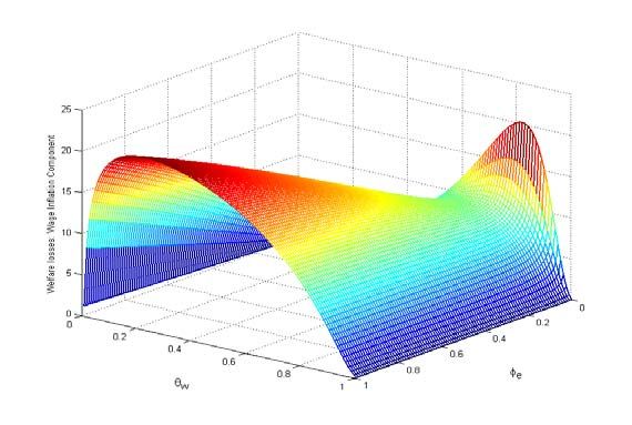
Figure 4 displays the three components of the welfare loss function, each being asso-
ciated with one of the three terms in (16). The graph for the …rst component, associated
19
The derivation of the welfare loss function (to be written up) combines elements of the derivations
of the corresponding function in Galí-Monacelli (2005) with those related to staggered-wage setting in
Erceg et al. (2000). See Campolmi (2012). The = 1 case, combined with our assumption of log utility
is a special case often referred to in the literature as the Cole-Obstfeld case.
20
We do not attempt to calibrate the variance of shocks, which we just normalize to unity. Thus, the
reader should not attach any weight to the absolute value of the welfare losses reported.
18with employment gap ‡uctuations, shows that an increase in wage ‡exibility always re-
duces the contribution of that component to overall welfare losses. Yet, it is clear that
the size of the reduction of the losses associated with that component is faster and more
prominent when e is zero or close to zero than when it is close to unity, a result con-
sistent with the …ndings of the previous section. Turning to the second component, we
observe that an increase in wage ‡exibility always raises the volatility of price in‡ation,
and thus the contribution of the latter to welfare losses. The size of that e¤ect seems
largely independent of the exchange rate policy.
Note that the wage in‡ation component of welfare losses displays the non-monotonicity
displayed by the overall loss, so its contribution is particularly important to account for
the …nding in Figure 3. The explanation for that non-monotonicity is straightforward. On
the one hand, and for any given e, the variance of wage in‡ation increases monotonically
as wages become more ‡exible. This e¤ect, which tends to raise welfare losses, is dominant
when w is relatively large thus accounting for the negative relationship between welfare
losses and that parameter over that upper range of the latter. On the other hand, the
weight associated with wage in‡ation volatility in the loss function, w= w, goes down
rapidly as wages become more ‡exible, accounting for the positive relation between welfare
losses and w when the latter parameter is below a certain level.21
Figure 5 splits the [ e ; w] parameter space in two regions, de…ned by the sign of the
impact of wage rigidities on welfare. The boundary between the two regions is given by the
value of w that maximizes welfare losses, as a function of e. Note that, as e increases,
i.e. as monetary policy becomes more focused on stabilizing the exchange rate, the range
of w values for which a (marginal) increase in wage ‡exibility is undesirable from a welfare
point of view becomes larger.22 In particular, in the limiting case of a hard peg or currency
union, an increase in wage ‡exibility is welfare improving only for values of w below 0:15,
21
Note that lim w !1 w = +1
22
One can further show that, for the = 1 case considered here, the boundary between the two regions
is invariant to the degree of openness.
19i.e. much lower than implied by the empirical evidence. Given that the weight w= w
is independent from e, the fact that the welfare losses are decreasing in w for a larger
range of values of the latter parameter when e is large must be related to the implied
behavior of wage in‡ation volatility. Thus, when e is low, the increase in wage volatility
resulting from an increase in wage ‡exibility is relatively small, compared to the case of
a high value of e. The change in the volatility of the "drivers" of wages –employment
and prices– resulting from greater wage ‡exibility is (relatively) more favorable to wage
stability when monetary policy is focused on stabilizing price in‡ation as opposed to the
nominal exchange rate.
Figures 6 through 8 report the corresponding …ndings when technology shocks are the
only source of ‡uctuations. Note that, qualitatively, the …ndings are very similar to those
obtained under the assumption of demand-driven ‡uctuations, though the boundary which
splits the two regions in the [ e ; w] parameter space now appears to be more sensitive to
the exchange rate coe¢ cient for low values of the latter.
We conclude this subsection by pointing out two additional …ndings, both of which
are captured in Figures 3 and 6. The …rst result has to do with the desirability or not of
some concern for exchange rate stability in the design of monetary policy. We note that,
independently of the value of w, the welfare loss function is minimized for some positive
(albeit small) value of e. In other words, and conditional on the assumed interest rate
rule (and given = 1:5), there are gains from having the central bank respond somewhat
to the nominal exchange rate, in order to dampen its ‡uctuations.23
Secondly, note that for a broad range of values of e (its entire support, in the case
of demand shocks), welfare losses for w = 1 (fully rigid wages) are smaller than those
associated with w = 0.(fully ‡exible wages).24 In both cases the component of welfare
23
That …nding is not unrelated to the conclusions of Campolmi (2012), who shows that CPI in‡ation
targeting is often more desirable than domestic in‡ation targeting in a model similar to ours. Note that
CPI in‡ation is a weighted average of domestic in‡ation and the change in the (log) nominal exchange
rate in our framework.
24
We thank our discussant, Stephanie Schmitt-Grohe, for pointing out this …nding.
20losses associated with wage in‡ation volatility is zero. Instead, we see that the gap in
welfare between the two extreme environments associated with price in‡ation volatility
(which favors fully sticky wages) more than o¤sets the corresponding gap associated with
employment gap volatility (which favors fully ‡exible wages). That result thus hinges
on the large weight associated with price in‡ation (relative to that of the employment
gap) in the welfare loss function under our baseline calibration, and can be overturned
when greater price ‡exibility is assumed. Moreover, the previous result is not invariant to
the speci…c monetary policy rule assumed. In particular, conditional on the central bank
following an optimal monetary policy, welfare losses are zero in the case of fully ‡exible
wages, but strictly positive when wages display some stickiness (even if not full), at least
as long as prices are sticky as well.25
4.2 Wage Flexibility, Exchange Rate Policy and Welfare: Ro-
bustness
In the present subsection we analyze the sensitivity of our …ndings to a variety of depar-
tures from the baseline calibration studied above. In particular, we investigate the role
of (a) the elasticity of substitution between domestic and foreign goods, (b) the degree of
openness, and (c) the degree of price stickiness.
4.2.1 The Role of the Trade Elasticity
The analysis above was restricted to a speci…cation of preferences featuring a unitary
value for the elasticity of substitution between domestic and imported goods (the trade
elasticity, for short), as well as a logarithmic utility of consumption. A recent literature
has shown that in the more general case - either because utility is not logarithmic or the
trade elasticity is di¤erent from 1 - it is no longer feasible to derive an accurate second
order approximation of households’welfare based only on a …rst order approximation of
25
The optimal monetary policy in the case of ‡exible wages is known to involve strict domestic in‡ation
targeting, i.e. H;t = 0, for all t. See Galí and Monacelli (2005).
21the underlying equilibrium conditions.26
In this subsection, we analyze the e¤ects of variations in the degree of wage rigidity on
welfare, and their interaction with the exchange rate policy, under alternative settings of
the trade elasticity. For concreteness, we restrict our analysis to the case of demand-driven
‡uctuations.
Throughout we continue to assume log-consumption utility. We evaluate the expected
discounted utility (loss) of the representative agent by resorting to a second-order ap-
proximation of the equilibrium conditions. In particular, we measure expected welfare
as: (1 )
X
t
Wt = Et U (Ct+k ; Nt+k ; Xt+k ) (17)
k=0
or, in recursive form:
Wt = U (Ct ; Nt ; Xt ) + Et fWt+1 g (18)
To evaluate the welfare level associated to alternative combinations of policy parame-
ters, we follow Schmitt-Grohe and Uribe (2004) and compute a numerical, second order
approximation of Wt . In turn, this requires computing a second order accurate approxi-
mation to the full set of equilibrium conditions.27
Figure 9, analogous to Figure 3 above, displays the e¤ect on welfare losses of varying
the degree of wage stickiness under alternative values of the exchange rate feedback coe¢ -
cient e. The …gure has two panels, corresponding to two di¤erent values of the elasticity
of substitution: = 0:5 ("low elasticity") and = 2 ("high elasticity"). Note that in
both cases the shape of the welfare loss function is qualitatively similar to that shown
in Figure 3. In particular, two of our main …ndings carry over to the two alternative
calibrations. Firstly, given an initial value of w is su¢ ciently low, making wages more
‡exible reduces welfare. Secondly, the range of w values for which more wage ‡exibility
26
See, e.g. de Paoli (2009).
27
See Schmitt-Grohe and Uribe (2004, 2007) for details.
22is welfare reducing increases with the size of the exchange rate coe¢ cient, and it is largest
in the case of an exchange rate peg or a currency union.
4.2.2 The Role of Trade Openness
Figure 10 shows the e¤ect of the exchange rate coe¢ cient e on the threshold value for
w under three alternative values for the openness parameter (0:1; 0:3; and 0:5). Once
again we report results for the case of demand shocks only.
We display results for two di¤erent calibrations of the trade elasticity, = 2 (panel
(a)) and = 1=2 (panel (b)). Under a unitary trade elasticity (not shown), the degree of
openness does not have any e¤ect on the threshold value of w and hence on the boundary
between the two welfare impact regions, which thus corresponds to that shown in Figure
5. In the case of non-unitary trade elasticities, and as Figure 10 makes clear, the degree
of openness a¤ects the welfare impact regions. Yet, we note that in both cases considered
the threshold value for w is decreasing in e, independently of the degree of openness.
Thus, a key …nding from the previous sections is shown to be robust to di¤erent degrees
of openness, even in the case of non-unitary trade elasticities.
Beyond that basic result, we note that the sign of the e¤ect of openness on the welfare
regions turns out to depend on whether that elasticity is larger or smaller than unity.
Thus, when = 2, greater openness reduces the size of the region for which welfare losses
are decreasing in w, for any given value of e (see Figure 10.a). The opposite e¤ect
obtains when = 1=2. In both cases, however, the e¤ect is relatively small.
4.2.3 The Role of Price Stickiness
The analysis of the previous sections has been conducted under the assumption of an
unchanged degree of price stickiness ( p = 0:75), corresponding to prices having an average
duration of four quarters: Figure 11 illustrates the e¤ect on the welfare impact regions of
varying the degree of price stickiness, conditional on both demand and technology shocks
23separately. In addition to the baseline value, we consider three alternative values (0:25,
0:5, and 1).
Consider …rst the case of demand-driven ‡uctuations. Notice that, with the exception
of the case of full price rigidity ( p = 1), the threshold value for w is generally decreasing in
the exchange rate feedback coe¢ cient e. As we approach full price rigidity, however, that
threshold value becomes independent of e. In other words, when prices are completely
rigid, it is irrelevant whether monetary policy is constrained or not, because domestic
in‡ation will not react to the underlying disturbances and, as a result, neither will the
nominal interest rate, given the assumed monetary policy rule (4).
Similarly, if prices are su¢ ciently ‡exible, the threshold value for wage stickiness is
also largely independent of e. In that case, in fact, it is irrelevant whether or not
monetary policy is unconstrained, because its ability to in‡uence the real interest rate,
via movements of the nominal interest rate, is impaired. Thus, in this vein, fully rigid
and fully ‡exible prices are symmetric cases. Note, however, that the relative size of the
welfare impact regions is very di¤erent in the two cases. In particular, the range of w
values for which welfare declines in response to greater wage ‡exibility tends to be larger
when prices are stickier, for any given value of e: Thus, and for any given e, an increase
in wage ‡exibility is more likely to be welfare improving when prices are relatively ‡exible.
In the case of technology shocks, a qualitatively similar pattern emerges, with the
boundary between the welfare impact regions being independent of e either at extreme
values of price stickiness or of price ‡exibility. Outside this parameter regions, and as
illustrated in our previous section, the threshold value for wage stickiness is decreasing in
the the exchange rate coe¢ cient e, although it becomes extremely sensitive to e at low
values of the latter.
The previous …nding suggests that the potential gains from greater wage ‡exibility
may be ampli…ed by a simultaneous increase in price ‡exibility. In order to asses that
conjecture we compute welfare losses (again, conditional on demand shocks) as a function
24of e and w under the additional constraint that p = w, i.e. that both price and wage
stickiness vary together. Figure 12 plots the resulting welfare loss function, conditional
on demand and technology shocks separately. Note that even though the overall shape of
the welfare loss function is qualitatively similar to that in Figures 3 and 6, the range of w
values for which the loss function is decreasing in that parameter is considerably smaller,
especially in the case of technology shocks. Furthermore, those losses converge to a value
to zero as both prices and wages approach full ‡exibility, independently of exchange rate
policy (since in the limiting case monetary policy is neutral).
The previous …nding thus suggests that, independently of the exchange rate policy, a
reduction in the degree of wage rigidities will be welfare improving if (i) it is large enough,
and (ii) is accompanied by a parallel increase in price ‡exibility.
5 Related Literature
Friedman (1953) is classic reference on the interaction between nominal rigidities and the
exchange rate regime. His "case for ‡exible exchange rates" rests on the usefulness of
exchange rate adjustments as a substitute for nominal price and wage adjustments, when
the latter are di¢ cult to bring about, in order to support a desirable or warranted change
in the relative price of domestic and foreign goods. The presence of su¢ ciently ‡exible
wages and prices as one of the criteria for the success of a currency union can be viewed
as a corollary of Friedman’s argument (see, e.g. European Commission (1990), Mongelli
(2002)). More recent theoretical work focusing on the costs of downward nominal wage
rigidity under an exchange rate peg can be found in Schmitt-Grohé and Uribe (2012),
among others.
A number of contributions have analyzed the consequences and desirability of increased
price and wage ‡exibility in the closed economy. Thus, DeLong and Summers (1986)
use a model with staggered Taylor contracts to show that a increase in wage ‡exibility
(indexed by the responsiveness of wages to cyclical conditions) may be destabilizing due
25to a Mundell e¤ect (i.e. the contractionary impact of falling prices, working through the
expected real rate).
Using a New Keynesian model, Battarai, Eggertsson, Schoenlen (2012) study the
conditions under which an increase in price ‡exibility may have destabilizing e¤ects on
output and employment. This will be the case if demands shocks are prevailing and
interest rates do not respond strongly to in‡ation. By contrast, when supply shocks are
dominant, greater price ‡exibility is destabilizing only if interest rates respond strongly to
in‡ation. Galí (2013) addresses the same question with a focus on wage ‡exibility and its
impact on welfare. He shows that an increase in wage ‡exibility may be welfare reducing
if the interest rate is not too responsive to in‡ation. The three papers rely on a closed
economy framework, and hence have nothing to say regarding the role of exchange rate
policy.
The constraints on monetary policy imposed by a currency union are similar to those
implied by a binding zero lower bound on the nominal interest rate.28 In that context,
Eggertsson, Ferrero and Ra¤o (2013) raise a warning on the possible contractionary ef-
fects of structural reforms (modelled as favorable supply shocks), due to the increase in
real interest rates resulting from de‡ationary pressures combined with an unresponsive
nominal rate.
6 Concluding Remarks
Calling for greater wage ‡exibility as a way of insulating employment from shocks has
become part of the conventional policy advice kit. For countries under a hard peg or
belonging to a currency union, wage ‡exibility is seen as being even more valuable, given
the impossibility of using the exchange rate as a bu¤er.
The present paper calls into question that conventional wisdom. Using a standard
New Keynesian open economy model, we have analyzed the impact of changes in the
28
Similar, but not identical, as made clear by Erceg and Lindé (2012).
26degree of wage rigidity on the economy’s equilibrium properties. Two …ndings stand out.
Firstly, the e¤ectiveness of labor cost adjustments on employment is inversely related
to the degree to which the central bank seeks to stabilize the exchange rate. That e¤ec-
tiveness is minimal in a currency union.
Secondly, an increase in wage ‡exibility often reduces welfare, and more likely so in
economies under an exchange rate peg or an exchange rate-focused monetary policy.
Our …ndings thus call into question the common view that wage ‡exibility is particu-
larly desirable in a currency union.
27APPENDIX
A.1. Households
The optimal allocation of any given expenditure on domestic goods yields the demand
functions:
p
PH;t (j)
CH;t (j) = CH;t (19)
PH;t
R1 1
1
p
for all j 2 [0; 1], where PH;t 0
PH;t (j)1 p
dj is the domestic price index. Com-
bining the optimality conditions in (19), with the de…nitions of PH;t and CH;t we obtain
R1
0
PH;t (j)CH;t (j)dj = PH;t CH;t .
The optimal allocation of expenditures between domestic and imported goods in turn
requires
CH;t = (1 )(PH;t =Pt ) Ct ; CF;t = (PF;t =Pt ) Ct (20)
1
where Pt ((1 )PH;t 1 + PF;t 1 ) 1 is the consumer price index (CPI, for short).29
Accordingly, total consumption expenditures by each household are given by PH;t CH;t +
PF;t CF;t = Pt Ct . Note that in a symmetric steady state with PH =P = 1 parameter
corresponds to the share of domestic consumption allocated to imported goods. It is also
in this sense that can be interpreted as an index of openness.
The household’s intertemporal optimality condition takes the form
Ct Xt+1 Pt
1 = (1 + it )Et
Ct+1 Xt Pt+1
where it is the interest rate on a one-period nominally riskless bond denominated in
domestic currency.
We assume a complete set of state-contingent securities traded internationally. That
29
When = 1 we have Pt (PH;t )1 (PF;t )
28assumption implies a risk sharing condition of the form:30
Ct = #Xt Ct Qt
Et Pt
where Qt Pt
is the real exchange rate and Ct is world consumption.31 Without
Et Pt
loss of generality we set # 1. Letting St PH;t
denote the terms of trade, note that
1
St = Qt (Pt =PH;t ) implies the monotonic relation Qt = St (1 ) + St1 1
.32
Each household is specialized in the provision of some di¤erentiated labor service,
for which …rms generate an isoelastic demand (see below) and for which each household
sets the corresponding nominal wage. Each period only a fraction 1 w of households,
drawn randomly from the population, reset their nominal wage in a way consistent with
utility maximization, subject to the demand for their labor services (current and future).
The remaining fraction w of households keep their nominal wage unchanged. Parameter
w 2 [0; 1] can be thus seen as an index of nominal wage rigidities.
The wage newly set in period t, denoted by W t , must satisfy the optimality condition:
X
1
Wt
k
( w) Et Nt+kjt Uc;t+k Mw M RSt+kjt =0 (22)
k=0
Pt+k
30
To see this note that
Et Vt;t+1 Xt Xt+1 Et+1
= t;t+1 (21)
Pt Ct Ct+1 Pt+1
Vt;t+1 1 1 1
= t;t+1
Pt Ct Ct+1 Pt+1
where Vt;t+1 is the period t price (in foreign currency) of a one-period (Arrow) security that yields one
unit of foreign currency if a speci…c state of nature is realized in period t + 1, and nothing otherwise, and
where t;t+1 is the probability of that state of nature being realized in t + 1 (conditional on the state of
nature at t).
31
Note that the equilibrium price of a riskless bond denominated in foreign currency is given, via arbi-
trage, by (1 + it ) 1 = Et fVt;t+1 g. The previous pricing equation can be combined with the corresponding
domestic bond pricing equation, (1 + it ) 1 = Et fVt;t+1 EEt+1t
g to obtain, after log-linearization, a familiar
version of the uncovered interest parity condition:
it = it + Et f et+1 g
32
When = 1 then Qt = St1
29'
where Mw w
w
1
is the frictionless wage markup and M RSt+kjt Ct+k Nt+kjt , with
'
Nt+kjt denoting t + k employment for a household who last set its wage in period t:
Log-linearization of the previous condition yields
X
1
w k
wt = + (1 w) ( w ) Et mrst+kjt + pt+k
k=0
w
where log Mw .
De…ne the economy’s average marginal rate of substitution as M RSt Ct Nt' , where
Nt is aggregate employment. Thus, up to a …rst order approximation,
mrst+kjt = mrst+k + '(nt+kjt nt+k ) (23)
= mrst+k w '(wt wt+k )
Furthermore, log-linearizing the expression for the aggregate wage index around a zero
in‡ation steady state we obtain
wt = w wt 1 + (1 w )w t (24)
We can …nally combine equations (22) through (24) and derive the baseline wage
in‡ation equation
w w w w
t = Et f t+1 g w( t ) (25)
w w
where t wt wt 1 is wage in‡ation, t wt pt mrst denotes the (log) average
(1 w )(1 w)
wage markup, and w w (1+ w ')
> 0.
A.2 Firms
Cost minimization by …rms implies a set of demand schedules for labor services of each
type:
w
W (i)
Nt (i; j) = Nt (j)
Wt
30You can also read