Benthic Megafaunal Community Structure and Biodiversity Along a Sea Ice Gradient on the Western Antarctic Peninsula: Insights into Climate Warming
←
→
Page content transcription
If your browser does not render page correctly, please read the page content below
Benthic Megafaunal Community Structure
and Biodiversity Along a Sea Ice Gradient
   on the Western Antarctic Peninsula:
     Insights into Climate Warming

                  A THESIS SUBMITTED TO
           THE GLOBAL ENVIRONMENTAL SCIENCE
      UNDERGRADUATE DIVISION IN PARTIAL FULFILLMENT
         OF THE REQUIREMENTS FOR THE DEGREE OF

                  BACHELOR OF SCIENCE

                             IN

             GLOBAL ENVIRONMENTAL SCIENCE

                       AUGUST 2010

                             By
                      Christian E. Clark

                       Thesis Advisors
                       Craig R. Smith
                        Laura Grange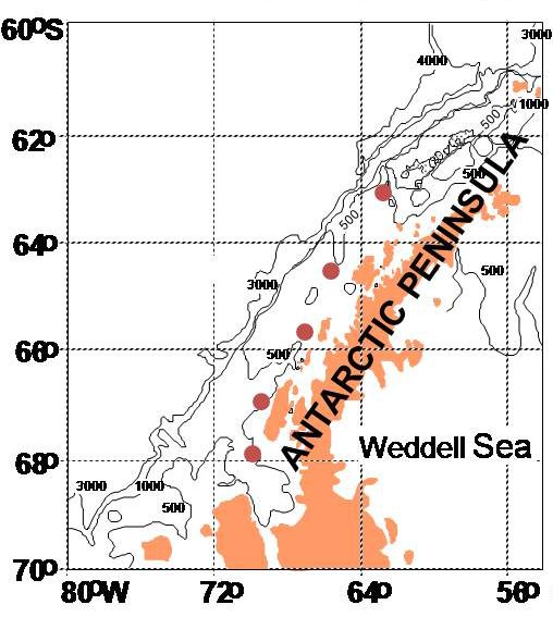
We certify that we have read this thesis and that, in our opinion, it is
    satisfactory in scope and quality as a thesis for the degree of
       Bachelor of Science in Global Environmental Science.

                                           THESIS ADVISORS

                                   ________________________________
                                              Craig R. Smith
                                        Department of Oceanography

                                   ________________________________
                                             Laura Grange
                                       Department of Oceanography

                                   ii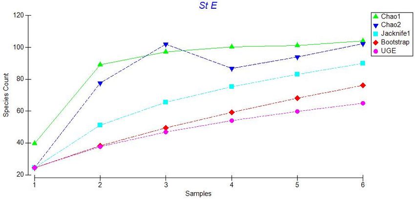
ACKNOWLEDGMENTS

       I would like to acknowledge the National Science Foundation for funding, the

captain and crew of the AS/RV Laurence M. Gould and RV/IB Nathaniel B. Palmer, the

United States Antarctic Program and Raytheon Polar Services for help with logistical

support and sample collection, everyone from North Carolina State University for their

help with sample collection and ship morale, my advisors Craig R. Smith and Laura

Grange, all members of the Smith Laboratory, Rhian Waller for help with species

identification, and the entire Global Environmental Science family: Jane Schoonmaker,

Rene Tada, Nancy Koike, Leona Anthony, and classmates.

                                           iii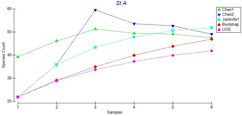
ABSTRACT

               The Western Antarctic Peninsula (WAP) is experiencing some of the

fastest rates of regional warming in the world, resulting in the collapse of ice shelves,

warming ocean temperatures, and increased melt and retreat of glaciers. Winter sea ice

coverage in the waters off the WAP has decreased in duration and extent over the last half

century. The significant changes observed off the WAP are extremely important in

studying the effects that global climate change may have on marine ecosystems.

Observed changes in sea ice may have negative effects on benthic ecosystems due to

interactions between sea ice, primary production, and pelagic-benthic coupling. The

effects of sea ice duration on deep benthic community structure (550-650 m depth) along

the WAP continental shelf are not well understood. We evaluated megafaunal abundance,

species richness, and community structure at five physically similar midshelf stations

along a strong latitudinal sea ice gradient from Smith Island (63S) to Marguerite Bay

(68S). Data collection included replicate towed “Yoyo Camera” transects (i.e.

quantitative photographic surveys) of the seafloor at each station. Our most northern

station (Sta. AA) experiences ~1 month of sea ice per year and our most southern station

(Sta. G) sees >7 months of sea ice cover per year. This study found that both megafaunal

abundance and community structure varied latitudinally along our north-south transect on

the WAP in concert with sea ice duration. Interestingly, species richness showed no

general patterns or trends as a result of sea ice extent. These results suggest that sea ice

                                              iv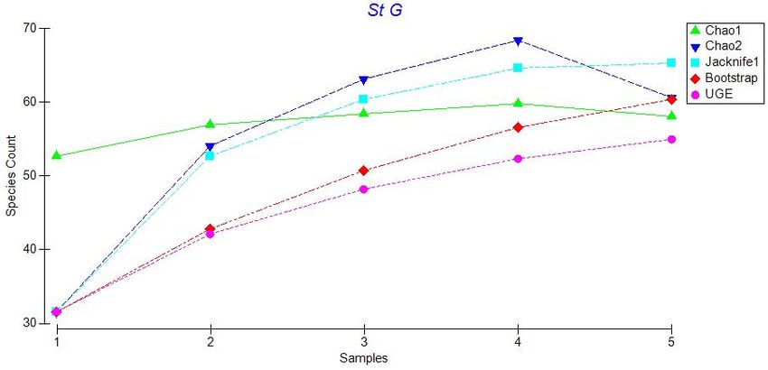
loss is likely to alter megabenthic community structure on the WAP, possibly causing a

shift from deposit-feeder dominated to suspension-feeder dominated communities along

the southern WAP.

                                           v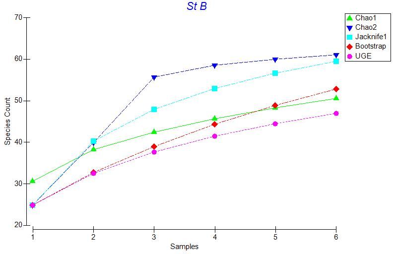
TABLE OF CONTENTS

Acknowledgments..............................................................................................................iii

Abstract...............................................................................................................................iv

List of Tables....................................................................................................................viii

List of Figures.....................................................................................................................ix

List of Abbreviations...........................................................................................................x

Chapter 1: Introduction........................................................................................................1

           1.1. Climate Change in Antarctica………………………………………………..1

           1.2. Bentho-pelagic Coupling…………………………………………………….2

           1.3. Labile Organic Matter Food Bank…………………………………………...3

           1.4. WAP Benthic Megafaunal Abundance, Species Richness, and Community

                  Structure…………………………………………….………………………..4

Chapter 2: Methods and Materials.......................................................................................7

           2.1. Experimental Design........................................................................................7

           2.2. Photographic Survey Methods.........................................................................9

           2.3. Data Processing………………………..........................................................12

           2.4. Statistical Analysis.........................................................................................14

Chapter 3: Results..............................................................................................................15

           3.1. Abundance…………………………...………………………….…………..15

                      3.1.1. Mean Abundance per m2.…………………………………………15

                      3.1.2. Statistical Results for Abundance……………………………..….16

                                                                   vi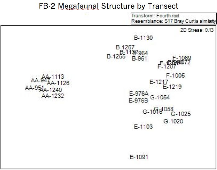
3.1.3. Most Abundant Species……………………………………….…..18

          3.2. Species Diversity………………....................................................................20

                      3.2.1. Species Richness and Accumulation……………………………...20

                      3.2.2. Evenness and Rarefaction………………………………………...24

          3.3. Community Composition…………………………………………………...26

                      3.3.1. Community Structure between Transects and Stations…………...26

                      3.3.2. Functional Groups………...............................................................28

Chapter 4: Discussion........................................................................................................30

          4.1. Abundance…………………………………………………….…….............30

          4.2. Species Richness……………………………………………………………33

          4.3. Community Composition and Trophic Structure…………………………...37

          4.4. Conclusion………………………………………………………………….39

Appendix............................................................................................................................40

References..........................................................................................................................43

                                                                 vii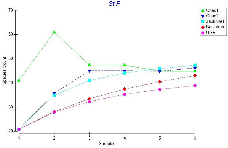
LIST OF TABLES

Table                                                             Page Number

Table 2.1: Table of Number of Images Analyzed for each CRS# and Station….………13

Table 3.1: Mean Abundance per m2………………………………….………………….15

Table 3.2: P-values for Mann-Whitney Test of Abundances……….…………………...17

Table 3.3: Top 10 Most Dominant Species at each Station……………………………..19

                                     viii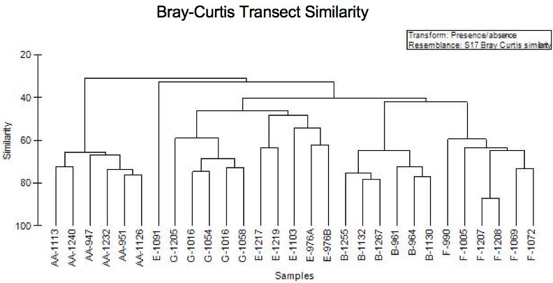
LIST OF FIGURES

Figure                                                    Page Number

Figure 2.1: Map of Sampling Stations along the WAP………………………………..…8

Figure 2.2: Mean Annual Sea Ice Cover for each Station………………………………..9

Figure 2.3: Yoyo Camera………………………………………………………………..10

Figure 3.1: Mean Abundances per m2……………………………………….…..………16

Figure 3.2: Species Accumulation Curves, Station AA…………………………………21

Figure 3.3: Species Accumulation Curves, Station B…………………………...………21

Figure 3.4: Species Accumulation Curves, Station E…………………………………...22

Figure 3.5: Species Accumulation Curves, Station F…………………………………...22

Figure 3.6: Species Accumulation Curves, Station G…………………………………..23

Figure 3.7: Chao 1 Estimator……………………………………………………………24

Figure 3.8: Rarefaction by Station………………………………………………………25

Figure 3.9: Evenness for each Station…………………………………………………..26

Figure 3.10: FB-2 Megafaunal Structure MDS Plot..….………………………………..27

Figure 3.11: Bray-Curtis Transect Similarity…………………………………………...28

Figure 3.12: Functional Group Composition by Station………………………………..29

                                  ix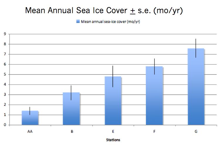
LIST OF ABBREVIATIONS

WAP:         Western Antarctic Peninsula

K:           Kelvin

AASW:        Antarctic Surface Waters

ACC:         Antarctic Circumpolar Current

CDW:         Circumpolar Deep Water

POM:         Particulate Organic Matter

POC:         Particulate Organic Carbon

ºC:          Degrees Celsius

Chl a:       Chlorophyll a

S:           South

m:           Meter

FOODBANCS:   Food for the Benthos on the Antarctic Continental Shelf

FB-2-1:      FOODBANCS 2 Cruise 1

FB-2-2:      FOODBANCS 2 Cruise 2

FB-2-3:      FOODBANCS 2 Cruise 3

AS/RV-LMG:   Antarctic Supply and Research Vessel Laurence M. Gould

RV/IB-NBP:   Research Vessel Ice Breaker Nathaniel B. Palmer

mm:          millimeter

cm:          Centimeters

CRS#:        CRS Number – unique deployment number

                                  x
m2 : Meters squared
s: Second
km: Kilometer
TIFF: Tagged Image File Format
Sta.: Station
Stas.: Stations
v.: Version
sp.: Species
UGE: Ugland Curve
Es: Expected species
nMDS: Nonmetric Multidimensional 4th Root Scaling plot
m/so: Mobile, Suspension Feeder
s/so: Sessile, Scavenger/Omnivore
m/sf: Mobile, Suspension Feeder
s/sf: Sessile, Suspension Feeder
m/df: Mobile, Deposit Feeder
s/df: Sessile, Suspension Feeder
m/c: Mobile, Carnivore
xiCHAPTER 1: INTRODUCTION
1.1. Climate Change in Antarctica
The Antarctic Peninsula is experiencing some of the fastest rates of regional
warming in the world and it is resulting in the collapse of ice shelves, warming ocean
temperatures, and the increased melt and retreat of glaciers (Clarke et al. 2007). This
rapid regional warming of the Antarctic Peninsula has resulted in the loss of at least seven
major ice shelves in the last 50 years (Vaughn and Doake 1996). Accompanying these ice
shelf collapses is decreased winter sea ice coverage. Regional winter sea ice coverage in
the Bellingshausen and Amundsen seas, off the Western Antarctic Peninsula (WAP), has
decreased in seasonal duration and in extent by almost 10% per decade for the last 50
years (Clarke et al. 2007). Subsequently in each of these two areas the mean annual air
temperature has increased by 1.5 K in the same period of time, compared to a global
increase of 0.6 K (Clarke et al. 2007).
The significant changes observed off the WAP are extremely important in
studying the effects that global climate change may have on marine ecosystems and
major earth systems. The WAP is the only area of Antarctica to show such a significant
decrease in seasonal sea ice extent and duration (Clarke et al. 2007). The trend of
decreased sea ice coverage and duration in the seas off the WAP may have negative
effects on marine and benthic ecosystems due to the unique interactions of the benthic
and pelagic environments on the Antarctic continental shelf.
1There are three characteristics of the Antarctic Surface Waters (AASW) of the
WAP that are responsible for the unique coupling of environments: exchange with the
atmosphere, sea ice coverage and duration, and interaction with the Antarctic
Circumpolar Current (ACC) carrying Circumpolar Deep Water (CDW) (Smith & Klinck
2002). The Antarctic continental shelf is remarkably deep compared to most continental
shelves. For most continental shelves the shelf is located within, or close to, the depth of
the seasonal mixed layer, which is not the case for the Antarctic continental shelf (Clarke
et al. 2007). This is a unique situation and as a result most of the continental shelf is
located below the depth of AASW. The fact that the continental shelf is located so deep
is important since it is suggested that the deep water of the ACC is warming much faster
than the mean rate calculated for the global ocean (Barnet et al. 2005, Clarke et al. 2007).
Increased warming could have significant impacts on marine ecosystems and their ability
to cycle nutrients.
1.2. Bentho-pelagic Coupling
All of the different variables associated with the WAP lead to an interesting
bentho-pelagic ecosystem on the continental shelf. The bentho-pelagic coupling
discussed in this paper will mainly focus on the downward coupling, in which the water-
column processes exert control on the benthos. There is a great deal of evidence that
suggests that bentho-pelagic coupling can considerably influence material cycles,
community dynamics, and fisheries yields in shelf ecosystems (Smith et al. 2006).
Bentho-pelagic coupling is accomplished off the WAP by seasonal fluxes of particulate
2organic matter (POM) raining down through the water-column providing food for key
components of the benthic food web, such as suspension feeders, deposit feeders, and
sediment microbes (Smith et al. 2006).
The environmental properties of the WAP shelf ecosystem determine the seasonal
variation of these POM fluxes to the benthic environment. These properties include:
summer and winter variations in sunlight, seasonal sea ice cover and its duration, and
water-column stratification. Taken together, these properties support development of
strong seasonality in pelagic primary production in Antarctica (Smith et al. 2006).
Seasonal variation in primary production causes distinct summer phytoplankton blooms,
which may cause higher export ratios and mass settling of phytoplankton to the benthos
during the summer season (Smith et al. 2006). Sinking and settling of organic material to
the shelf floor allows for the development of benthic communities. The composition and
size of benthic communities reflect the production processes of the waters above, and can
yield important insights into the climate-driven changes of coastal pelagic ecosystems.
1.3. Labile Organic Matter Food Bank
The highly climate-driven seasonal flux of particulate organic carbon (POC) to
the WAP shelf during the summer bloom allows for a large deposition of labile organic
material on shelf sediments, which supports benthic detritivores and microbial
assemblages (Mincks et al. 2005). However, despite its labile nature, the consistently low
bottom-water temperatures in the WAP (-2.0 to 1.0ºC) region may slow the metabolic
remineralization of organic material deposited on the shelf floor and allow it to be buried
3in the shelf sediments (Mincks et al. 2005, Nedwell 1999).
Mincks et al. (2005) suggested that a combination of increased particle sinking
rates and low-temperature inhibition of metabolic activity could cause a build-up and
storage of organic material in WAP sediments and lead to a long-term ‘food bank’ in shelf
sediments. Due to the large area extent of the Antarctic continental shelf, which covers
11% of the total area of continental shelf worldwide, the ability of WAP sediments to
sequester organic carbon in a sediment ‘food bank’ is extremely important in
understanding the community structure of benthic megafauna on the seafloor of the deep
continental shelf of the WAP (Clarke and Johnston 2003).
1.4. WAP Benthic Megafaunal Abundance, Species Richness, and Community
Structure
The rapid climate change seen along the WAP over the last half-century is
expected to continue if not increase in the future. In an area where marine ecosystems
are heavily dependent on sea ice extent, duration and seasonal phytoplankton blooms,
increased warming will likely play a key role in determining ecosystem structure. This is
primarily due to the likelihood for decreased sea ice duration in the coastal waters of the
WAP. In the long term, decreases in sea ice will likely cause increases in primary
production in the surface waters, due to increased light availability in a light limited
environment (e.g., Arrigo et al. 2008). This in turn, will alter the quantity and quality of
food availability to the coastal food web and modify phytodetrital rain down to the
benthos. These changes in quantity and quality of primary production will vary
4temporally and spatially, and are likely to influence long-term stability of the WAP
ecosystem.
In a recent study, Montes-Hugo et al. (2009), satellite observations were compiled
for Chlorophyll a (Chl a) concentrations in surface waters of the WAP as an indicator of
primary production levels. The study found that, when current satellite observations of
Chl a were compared to a baseline data set from 1978-1986, primary production levels
have indeed changed in the past thirty years (Montes-Hugo et al. 2009). In coastal waters
of the northern region of the WAP, primary production levels have dropped considerably
since the early 1980’s and have increased in surface waters of the southern WAP region
(Montes-Hugo et al. 2009). They attributed the decreases in the northern region to highly
reduced sea ice seasons where the lack of sea ice has allowed increased turbulent mixing,
increased cloudiness, and resulted in deeper mixed layers, thereby decreasing the
productivity of the waters by actually decreasing the exposure of primary producers to
light (Montes-Hugo et al. 2009). On the other hand, the surface waters of the southern
WAP appear to be sustaining greater primary production from shortened sea ice seasons,
more light availability, and increased mixing (Montes-Hugo et al. 2009).
Therefore, the relationship between, a reduction of sea ice and primary
productivity of the coastal waters may be complicated on shorter time and spatial scales,
destabilizing or at least altering WAP food webs (Montes-Hugo et al. 2009).
Consequently, changes in primary production along the WAP due to sea ice loss will most
likely change the structure of the coastal marine ecosystems. Decreased phytoplankton
blooms along the northern WAP appear to have substantially changed the pelagic food
5web (Montes-Hugo et al. 2009) and therefore altered food fluxes to the benthos, resulting
in less phytodetrital rain down. However, increased primary production along the
southern WAP has likely increased the amount of food availability and amplified food
fluxes to the benthos. These productivity changes, both positive and negative, are
expected to alter community structure from the bottom up.
Due to the central importance of sea ice extent and duration to the WAP
ecosystem this study will focus on changes to the benthos along a sea ice gradient along
the WAP shelf. The main questions that this study will address are: how does benthic
megafaunal abundance, community structure, trophic composition, and diversity vary
along a strong latitudinal sea ice gradient on the WAP continental shelf? We hypothesize
that megafaunal abundance, community structure and trophic composition, and species
biodiversity will vary latitudinally concomitantly with variations in sea ice extent and
duration.
6CHAPTER 2: METHODS AND MATERIALS
2.1. Experimental Design
In this study we worked at five physically similar mid-shelf stations along the
WAP continental shelf from approximately 63o S to 68o S. These stations all consisted of
soft sediment bottoms and low current regimes at depths from 550 m to 650 m, allowing
us to maintain relatively constant benthic habitat variables along a latitudinal gradient on
the WAP continental shelf. Stations were named alphabetically starting with station AA
our most northern station, station B, station E, station F, and station G our most southern
station located off of Marguerite Bay, as seen in Figure 2.1. This north-south transect
partially overlaps stations from a previous study, FOODBANCS, which assessed the
benthic community structure along an east-west transect sampling an inner shelf station
A, a mid-shelf station B (used also in this project), and an outer-shelf station C.
The orientation of our north-south transect allowed us to sample along a strong
sea ice gradient. Srsen et al. (unpublished data), shows that average annual sea ice
duration for the period 2004 - 2008 increases from north to south along our transect from
a minimum of 1.4 months per year at station AA to a maximum of 7.6 months per year at
station G (Figure 2.2). Stations were studied at three time points during two summer
cruises (cruises FB-2-1 and FB-2-3) aboard the Antarctic Supply and Research Vessel the
Laurence M. Gould (AS/RV-LMG), February to mid March of 2008 and 2009, and one
winter cruise (cruise FB-2-2) on the Research Vessel Ice Breaker Nathaniel B. Palmer
(RV/IB-NBP), from July to early August of 2009. The cruise schedule allowed us to
7sample during both winter and summer for comparisons of the benthic community
patterns across seasons and years. This is important when considering the large seasonal
differences in nutrient fluxes to the benthos along the WAP, which is characterized by
large fluxes during summer months and very little during winter months, as well as high
interannual variability (e.g., Smith et al. 2006).
AA
B
E
F
G
Figure 2.1: Sampling stations AA, B, E, F, and G located along the Western Antarctic
Peninsula (from Srsen et al., unpublished). Dots indicate sampling stations and the
Antarctic Peninsula is shown in solid color. Lines note 500-meter isobaths.
8Figure 2.2: Mean annual sea ice cover + standard error. Vertical blue bars indicate
months of sea ice cover per year for each of our five sampling stations (AA, B, E, F, and
G) based on satellite data from the National Snow and Ice Data Center (Srsen et al., un-
Published).
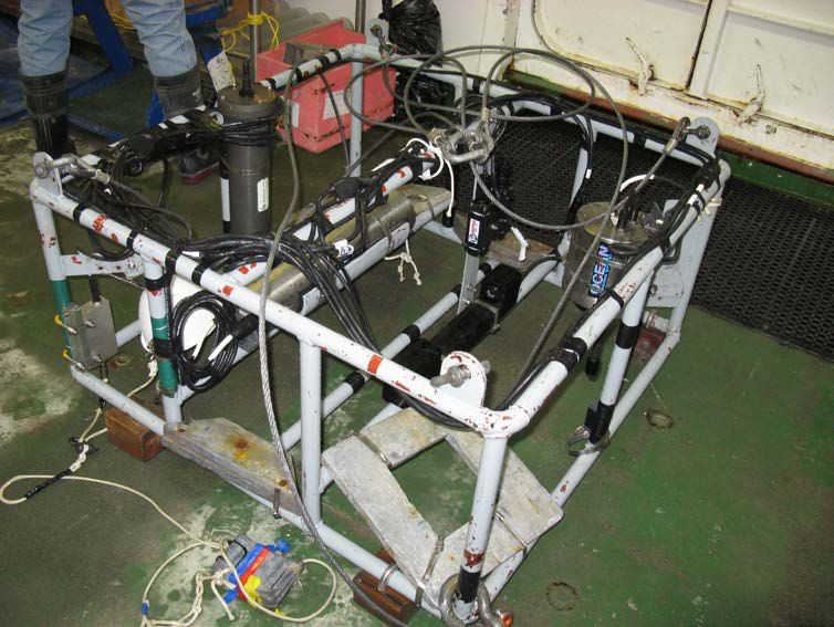
2.2. Photographic Survey Methods
Photographic surveys were conducted using a using a “Yoyo Camera” system
developed for the project. This consists of a vertically oriented camera with a strobe one
meter away, actuated by a bottom contact switch (Figure 2.3). The camera is an Ocean
Imaging Systems DSC 10000 digital still camera in titanium housing, with a 10.2 mega
pixel sensor and 20 mm Nikon lens. The Yoyo frame system also included a 200 watt-
second Ocean Imaging Systems 3831 Strobe, an Ocean Imaging Systems model 494
9bottom contact switch with weighted 1.5 m lanyard, and parallel red lasers for scaling.
The camera was mounted on the frame looking vertically downward, prior to every
deployment, with the underwater strobe offset by one meter, both were actuated with the
bottom switch. The scaling lasers were checked before each deployment to make sure
they were parallel and aimed directly downward 10 cm apart. The Yoyo Camera system
was also equipped with a transmissometer providing real time data on shipboard, and an
audible alarm, which sounded when the bottom contact switch closed, firing the camera.
This allowed us to collect images of the seafloor at a high rate without dragging the
camera or stirring up a large sediment cloud (resuspended sediment was detected by the
transmissometer).
Figure 2.3: Yoyo Camera frame pre-deployment stage aboard the RV/IB-NBP. Shown in
the image are the underwater camera (far right), strobe (far left), scaling lasers and
bottom contact switch (center), and weighted 1.5 m lanyard (bottom center).
10The survey method using the Yoyo Camera was the same across all stations and
cruises with only minor variations of deployment. The only variation in our survey
method was because of differences in deck the configurations of the RV/IB-NBP and the
AS/RV-LMG. The larger RV/IB-NBP was configured with both an aft A-frame winch
and starboard A-frame winch, while the smaller AS/RV-LMG was equipped with only an
aft A-frame winch. Consequently, on both of our cruises aboard the AS/RV-LMG the
camera frame was deployed from the aft A-frame winch, whereas during our austral
winter cruise on the RV/IB-NBP the bottom camera was deployed midship from the
starboard A-frame winch. Both methods worked well, however deployment from the
starboard winch proved to be more suitable for collecting bottom pictures because of the
reduced pitching motion midship.
Photo transects were completed at every station using the towed Yoyo Camera
system. Each transect was assigned a unique deployment number (CRS #) (Table 2.1).
Transects began at each station and proceeded in the best direction allowed by ice
conditions and wind, which essentially randomized transect headings. Using an A-frame
winch, the camera was lowered near to the seafloor and towed at a speed of ~1 knot. The
camera was then lowered until the bottom-contact switch fired, then raised ~1.5 m off the
seafloor and lowered again for the next firing. Each photo covered ~3 m2 of seafloor.
The time interval between photographs was about 15 s, yielding a spacing of 7 – 10 m
between the centers of consecutive photos. Transects were terminated after transiting a 1
km linear distance or once 100 images of the seafloor had been collected, whichever
came second. Replicate transects were completed at every station and on every cruise,
11with the exception of station G on our third cruise during which time constraints and
complications with the camera system allowed us to conduct only one transect of
replicate transects with less than 100 usable images.
2.3. Data Processing
Images collected during this study were color corrected, based on in situ images
of a red-green-blue-white color chart, using Adobe ImageReady software. During our
first cruise an Adobe ImageReady “droplet” (or mini-program) was created to correct the
colors of the chart when photographed at depth during the first photo transects.
Subsequent pictures taken on each cruise were color corrected using this droplet to adjust
the proper color balance at depth (uncorrected images were heavily blue biased). This
enabled us to exploit the high resolution of the camera and enhanced our abilities to
distinguish animals, bioturbation features, and details in each image that would have been
lost without color correction.
After color correction, bottom images were then imported as high-resolution jpegs
into ImageJ software for scaling. Each individual picture was scaled in ImageJ using the
10 cm laser spots on the seafloor. Once an image was scaled it was saved as a TIF file so
that the image scale, specific to each picture, was permanently attributed to that file as
part of the image information (scaling is not saved in the jpeg file format). This allowed
the file to be scaled only once and avoided the human error that would have been
associated with having to rescale a jpeg file every time it was opened.
Following scaling in ImageJ, a 20 x 20 cm grid was overlain over each photo to
12add a representative scale for animals in each image and aid in the compilation of an
animal identification photo atlas. When an organism was found, a screen grab was taken
of the animal. Screen grabs were then taken of exemplary and identifiable species in
every image for all stations and cruises. After the compilation of the photo atlas, animals
were identified and named using literature and reference material from trawl samples
taken at every station.
Once photo atlases were completed for each station and a global photo atlas was
compiled, animal counts for each CRS # were conducted using ImageJ’s cell counter. A
30 x 30 cm grid was overlain on each photo and a count area of 1.8 m2 in the center of
each image was analyzed. Of the 100 or more images collected on each replicate photo
transect, we randomly selected 50 photos for counting using an Excel random number
generator. Due to sediment clouds, the random photos were adjusted slightly so that all
the images counted had a clear central count area. This was not able to be accomplished
on all transects and three transects had less than 50 countable pictures; CRS #1207 Sta.F
cruise FB2-3 only had 46 countable pictures, CRS# 1208 Sta. F cruise FB2-3 had 43
countable pictures, and CRS #1205 (the only photo transect completed at Sta. G on cruise
FB2-3) yielded 23 countable images. In total, 1,412 bottom photos covering 2542 m2
were analyzed in this study (Table 2.1).
Table 2.1: Table of Number of Images Analyzed for each CRS# and Station
Station AA Image Count Station B Image Count Station E Image Count Station F Image Count Station G Image Count
CRS 947 50 CRS 961 50 CRS 976 (A) 50 CRS 990 50 CRS 1016 50
CRS 951 50 CRS 964 50 CRS 976 (B) 50 CRS 1005 50 CRS 1020 50
CRS 1113 50 CRS 1130 50 CRS 1091 50 CRS 1069 50 CRS 1054 50
CRS 1126 50 CRS 1132 50 CRS 1103 50 CRS 1072 50 CRS 1058 50
CRS 1232 50 CRS 1255 50 CRS 1217 50 CRS 1207 46 CRS 1205 23
CRS 1240 50 CRS 1267 50 CRS 1219 50 CRS 1208 43 N/A 0
Total: 300 Total: 300 Total: 300 Total: 289 Total: 223
Table 2.1: Table of the total number of bottom images analyzed for each photo transect
(CRS#) and station.
132.4. Statistical Analysis
Differences in abundance and species richness between stations and cruises were
compared using non-parametric Kruskal-Wallis and Mann-Whitney tests. These
statistical analyses were carried out using Minitab Statistical software v.15. Biodiversity
analyses and community comparisons were conducted using PRIMER 6 software.
Analyses conducted with PRIMER 6 included species accumulation plots by station
(Ugland curves), estimates of total species richness by station (Chao 1, Chao 2, Jacknife
and Bootstrap estimators), community similarity across all lowerings based on MDS
using 4th root transformations to include contributions from both common and rare
species, and Bray-Curtis Similarity.
14CHAPTER 3: RESULTS
3.1. Abundance
3.1.1. Mean Abundance per m2
A total of 17,469 individual benthic megafauna, and 111 nektonic individuals,
were counted in 1412 images. Station F had the highest densities of benthic megafauna
(individuals per square meter) with CRS# 1069 and CRS# 1072 having the most animals
per square meter of all transects, 13.89 per m2 and 14.10 per m2 respectively (Table 3.1).
CRS# 1103 (Sta. E) and CRS# 1205 (Sta. G) had the lowest in the lowest densities of
benthic megafauna of all transects with 1.77 and 3.77 individuals per m2 (Table 3.1).
Table 3.1: Mean Abundance per m2
STATION AA STATION B STATION E STATION F STATION G
Ind. Ind. Ind. Ind. Ind.
Transect Transect Transect Transect Transect
per m2 per m2 per m2 per m2 per m2
CRS 947 10.87 CRS 961 6.03 CRS 976 (A) 3.71 CRS 990 13.47 CRS 1016 4.28
CRS 951 9.72 CRS 964 5.91 CRS 976 (B) 3.73 CRS 1005 10.97 CRS 1020 3.74
CRS 1113 7.02 CRS 1130 4.47 CRS 1091 3.02 CRS 1069 13.89 CRS 1054 3.07
CRS 1126 7.60 CRS 1132 4.37 CRS 1103 1.77 CRS 1072 14.10 CRS 1058 3.10
CRS 1232 9.59 CRS 1255 6.07 CRS 1217 3.34 CRS 1207 9.09 CRS 1205 3.77
CRS 1240 11.10 CRS 1267 5.37 CRS 1219 2.69 CRS 1208 12.74 N/A N/A
Table 3.1: Table of mean abundance per meter squared for each photo transect. Transect
column indicates photo transect label while the Ind. per m2 column indicates average
number of individuals seen per transect in a one meter square area.
Mean abundance per m2 of each transect with standard error was then plotted by
station to evaluate variability between transects. Figure 3.1 gives a graphical
representation of the values in Table 3.1. For the most part, the abundances per m2 for
each transect did not vary much by station. Station AA and Station F had the largest
spread of mean abundance per m2 by transect, with differences of 5 - 7 individuals per m2
between maximum and minimum abundance values (Figure 3.1).
15Figure 3.1: Plot of mean abundances per m2 for each photo transect + standard error.
Each point indicates mean abundance per m2 for an individual transect. Transects were
then grouped by station to show mean abundance spreads between transects for each
station.
3.1.2. Statistical Results for Abundance
Statistical tests were completed to determine whether or not there were significant
differences in the mean megafaunal abundance per square meter between stations and
also between cruises. The results of a Kruskal-Wallis Test for total abundances between
stations showed that there were significant differences between stations (p = 0.000, H =
871.97, DF = 4). A Kruskal-Wallis Test of abundances between cruises also indicated
that there were significant differences between cruises (p = 0.000, H = 922.01, DF = 14).
Mann-Whitney tests were also carried out to determine whether or not there were
significant differences between stations and between cruises.
16The results of the Mann-Whitney Test between stations showed that were
significant differences between all stations (Table 3.2). Results from a Mann-Whitney
Test of abundances between cruises showed that there were no significant differences
between cruise FB-2-1 and FB-2-3 at Sta. AA (p = 0.4626), FB-2-1 and FB-2-3 at Sta. B
(p = 0.5938), FB-2-3 Sta. AA and FB-2-3 Sta. F (p = 0.1381), FB-2-2 Sta. B and FB-2-1
Sta. G (p = 0.0765), FB-2-2 Sta. B and FB-2-3 Sta. G (p = 0.0575), FB-2-1 Sta. E and
FB-2-1 Sta. G (p = 0.2103), FB-2-1 Sta. E and FB-2-1 Sta. G (p = 0.8525), FB-2-3 Sta. E
and FB-2-2 Sta. G (p = 0.8293), and FB-2-1 Sta. G and FB-2-3 Sta. G (p = 0.4029). A
full table of p-values between cruises is located in the Appendix.
173.1.3. Most Abundant Species
The ten most abundant species for each station were determined by their mean
abundance per square meter from all transects. Table 3.3 shows the 10 dominant benthic
megafauna at Sta. AA with Ophiuroid sp.2, Anemone sp.3, and Notocrangon antarcitcus
accounting for almost 90% of the total abundance at Sta. AA. The three most dominant
species at Sta. B were Chaetopterus sp., Ophiuroid sp.4, and Pycnogonid sp.2,
accounting for nearly 80% of the total abundance at Sta. B (Table 3.3). At Sta. E,
Chaetopterus sp., Ampheliscid amphipod sp.1, and Protelpidia murrayi, accounted for
approximately 75% of animals present (Table 3.3). Chaetopterus sp., Rhipidothuria
racowitzai, and Ampheliscid amphipod sp.1 made up close to 90% of the total abundance
of animals at Sta. F (Table 3.3). Sta. G’s dominant three species made up the lowest
percent of total abundance of all stations with Chaetopterus sp., Protelpidia murrayi, and
Ophiuroid sp.4 being responsible for only ~58% of Sta. G’s total abundance (Table 3.3).
Of the ten dominant species at each station, Notocrangon antarcticus was the only
species present at all stations while Chaetopeterus sp. was the most prevalent species at
Sta. B, E, F, and G. Mysid sp.1 was also prevalent at Sta. AA, B, and E but was excluded
from benthic megafaunal counts because it was always in the water column when
photographed.
18Table 3.3: Top ten most abundant species for each station
Station AA % Tot. Abundance Indiv. per m2
Ophiuroid sp.2 80.1 7.48
Anemone sp.3 5 0.47
Notocrangon antarcticus 4.3 0.4
Anemone sp.1 2.5 0.23
Isopod sp.1 1.6 0.146
Pycnogonid sp.1 1.4 0.13
Anthomastus bathyproctus 1.3 0.117
Ophionotus victoriae 0.6 0.056
Flabellum impensum 0.5 0.048
Anemone sp.2 0.4 0.033
Station B % Tot. Abundance Indiv. per m2
Chaetopterus sp. 72 3.89
Ophiuroid sp.4 3.3 0.178
Pycnogonid sp.2 3 0.161
Notocrangon antarcticus 2.9 0.156
Ascidian sp.3 2.5 0.133
Pycnogonid sp.1 2.4 0.126
Anemone sp.1 2.1 0.115
Ascidian sp.2 1.8 0.098
Isopod sp.1 1.3 0.07
Peniagone vignioni 1.2 0.063
Station E % Tot. Abundance Indiv. per m2
Chaetopterus sp. 56.4 1.72
Ampheliscid amphipod sp.1 12 0.365
Protelpidia murrayi 6.3 0.193
Notocrangon antarcticus 6 0.17
Juvenile Elasipod sp.1 4.5 0.137
Ascidian sp.3 1.3 0.041
Bolocera kerguelensis 1.2 0.037
Pycnogonid sp.1 1.1 0.033
Scaleworm sp.1 1 0.031
Ophiuroid sp.4 1 0.031
Station F % Tot. Abundance Indiv. per m2
Chaetopterus sp. 75 41.7
Rhipidothuria racowitzai 8.7 4.83
Ampheliscid amphipod sp.1 4.9 2.72
Protelpidia murrayi 4.5 2.5
Notocrangon antarcticus 1.9 1.06
Isopod sp.2 1 0.556
Peniagone vignioni 0.7 0.389
Pycnogonid sp.2 0.6 0.333
Isopod sp.1 0.6 0.333
Ophiuroid sp.5 0.5 0.028
Station G % Tot. Abundance Indiv. per m2
Chaetopterus sp. 32.3 1.15
Protelpidia murrayi 19.7 0.705
Ophiuroid sp.4 6.4 0.229
Juvenile Elasipod sp.1 5.9 0.212
Notocrangon antarcticus 5.3 0.189
Golf Sponge sp.1 4.7 0.169
Sponge sp.1 3.9 0.14
Peniagone vignioni 3.8 0.135
Ampheliscid amphipod sp.1 2.4 0.085
Bolocera kerguelensis 1.9 0.067
193.2. Species Diversity
There are two main components to species diversity: species richness, i.e. number
of species present, and evenness, i.e., how uniformly distributed individuals are among
species.
3.2.1. Species Richness and Accumulation
The number of species collected at a station is dependent on sample size, until the
full species list has been sampled. Thus, as transects were added and sample size
increased, the likelihood that more species would accumulate also increased. Therefore,
we used a variety of techniques to (1) determine that species were still accumulating at
each station, and (2) estimate total species richness for each station. To understand how
species diversity accumulated at each station as transects were added, we used an Ugland
curve (UGE) which provides the mean species accumulation per transect at each station,
based on 999 random orderings on of the transects (Figures 3.2 – 3.6).
As seen in Figure 3.2 to Figure 3.6 the UGE curve is still increasing at all stations
after all transects have been added. This indicates that species are still accumulating at
every station and we did not sample all of the species present at any station. Therefore,
we used multiple species richness estimators to compare species richness between
stations. The estimators we used to estimate total species richness at each station were
the Chao 1, Chao 2, Jackknife, and Bootstrap estimators, Figures 3.2 – 3.6.
20Figure 3.2: Plot of five species estimators for Station AA: Chao 1, Chao 2, Jacknife 1,
Bootstrap, and Ugland. Species counts refer to total number of species and samples
correspond to additional photo transects (i.e. sample 1 is the first transect, sample 2 is
transect 1 plus transect 2, etc.).
Figure 3.3: Plot of five species estimators for Station B: Chao 1, Chao 2, Jacknife 1,
Bootstrap, and Ugland. Species counts refer to total number of species and samples
correspond to additional photo transects (i.e. sample 1 is the first transect, sample 2 is
transect 1 plus transect 2, etc.).
21Figure 3.4: Plot of five species estimators for Station E: Chao 1, Chao 2, Jacknife 1,
Bootstrap, and Ugland. Species counts refer to total number of species and samples
correspond to additional photo transects (i.e. sample 1 is the first transect, sample 2 is
transect 1 plus transect 2, etc.).
Figure 3.5: Plot of five species estimators for Station F: Chao 1, Chao 2, Jacknife 1,
Bootstrap, and Ugland. Species counts refer to total number of species and samples
correspond to additional photo transects (i.e. sample 1 is the first transect, sample 2 is
transect 1 plus transect 2, etc.).
22Figure 3.6: Plot of five species estimators for Station G: Chao 1, Chao 2, Jacknife 1,
Bootstrap, and Ugland. Species counts refer to total number of species and samples
correspond to additional photo transects (i.e. sample 1 is the first transect, sample 2 is
transect 1 plus transect 2, etc.).
Figures 3.2 to 3.6 indicate that these estimators generally agree at all stations,
therefore we used Chao 1 for our comparisons. A plot of Chao 1 with + one standard
error shows that species richness is similar across all stations except Sta. E (Figure 3.7).
Station E has many species that occur as singletons (only one individual of that species
observed), giving a much higher and more variable value for the Chao 1species richness
estimator. Other species richness estimators also show a peak in species richness at Sta.
E, although this peak is less marked, especially for the Bootstrap estimator. Nonetheless,
for all the species richness estimators, there is no obvious latitudinal trend in estimated
species richness along the sampling transect.
23Figure 3.7: Plot of Chao 1 estimator values for all stations + standard error. The number
of species corresponds to the total number of species that could be expected at each
station with infinite sampling effort.
3.2.2. Evenness and Rarefaction
The second component of species diversity, evenness, can be assessed with two
metrics: (a) Rarefaction diversity, which evaluates both richness and evenness, and (b) J',
a strict species evenness index. Once again, evenness refers to how uniformly distributed
individuals are between species. The Rarefaction diversity for each station with the
expected number of species in a sub sample of 150 individuals, Es(150), is plotted in
Figure 3.8, and Evenness J' for each station is shown in Figure 3.9. Both indices show a
nearly latitudinal trend, however, Sta. F and Sta. AA have similarly low diversity indexes.
Mann-Whitney Tests were used to test for significant differences in the means of Es(150)
and Evenness J' values. There were no significant differences for the mean values for the
Es(150) index between Sta. AA and Sta. F (p = 0.4712), and Sta. B and Sta. E (p =
240.2298). The Mann-Whitney Test of the Evenness J' index indicated that there was no
significant difference between Sta. AA and Sta. F (p = 0.0927). Mann-Whitney p-value
tables for Es(150) and Evenness J' indices are located in Appendix.
Rarefaction by Station
30
25
20
Mean Es(150)
15
10
5
0
Sta. AA Sta. B Sta. E Sta. F Sta. G
Figure 3.8: Plot of Rarefaction for each station. Mean Es(150) values correspond to the
total number of species that would be expected in a sub sample size of 150 images for
each station.
25Evenness for each Station
0.8
0.7
0.6
Mean Evennes J'
0.5
0.4
0.3
0.2
0.1
0
Sta. AA Sta. B Sta. E Sta. F Sta. G
Figure 3.9: Plot of Evenness for each station. Evenness J’ values correspond to a
uniform distribution indicator value. Higher values indicate increased uniform
distribution of individuals between species present at each station and lower indicate
decreased uniform distribution (i.e. less biodiversity).
3.3. Community Composition
3.3.1. Community Structure
Community structure was compared between transects and stations using a non-
Metric Multidimensional Scaling analysis. The results from this analysis are plotted in
Figure 3.10. The results indicate that there three basic clusters: Sta. AA, Sta. B, and a
combined cluster of Sta. E, F, and G. This suggests Sta. AA is distinct from all other
stations in both species identifications and proportions. The separation distance of cluster
Sta. B, in Figure 3.10, indicates that Sta. B is very different from Sta. AA and only
somewhat different from the Sta. E, F, and G cluster. The MDS 4th root plot, Figure 3.10,
also suggests that there is a gradual shift in community structure along the sampling
transect from Sta. AA to Sta. G.
26Figure 3.10: Non-metric Multidimensional Scaling plot of species community structure
similarity between all transects. Three main clusters: Sta. AA, Sta. B, and Stas. E,F, and
G. Transect scaling is based on presence-absence data from Bray-Curtis index for each
transect.
The non-Metric Multidimensional Scaling (nMDS) analyses used a Bray-Curts
similarity index of presence-absence data to compare community structure across
transects. As seen in Figure 3.11, the abrupt changes in community structure between
Sta. AA, B, and E result from this similarity index and are due to the differences in
proportions and identities of species across stations. The Bray-Curts Similarity plot,
Figure 3.11, shows that stations share 30-40% of their species across the entire station
transect (Sta. AA-G.).
27Figure 3.11: Bray-Curtis plot of similarity between all photo transects. Similarity index
is based on presence-absence data for species at each station. Similarity values indicate
the percentage of species that are shared by each transect. Samples correspond to species
lists for individual transects (i.e. AA-1113 = Station AA CRS# 1113, etc.).
3.3.2. Functional Groups
Functional groups analyses were conducted by assigning all species counted in
this study, except for nekton, one of seven functional group labels based on locomotion
type and feeding characteristics. Functional groups were as follows: m/so (mobile,
suspension feeder), s/so (sessile, scavenger/omnivore), m/sf (mobile, suspension feeder),
s/sf (sessile, suspension feeder), m/df (mobile, deposit feeder), s/df (sessile, suspension
feeder), and m/c (mobile, carnivore). Functional group structure for each station was
then analyzed by examining the percent of the total individuals per station that each
functional group represented, as shown in Figure 3.12.
28Figure 3.12: Plot of functional group composition for each station. Percent of total
abundance corresponds to the percent of individuals for each functional group that make
up the total abundance at each station. Functional groups are: m/c (mobile carnivore),
s/df (sessile suspension feeder), m/df (mobile deposit feeder), s/sf (sessile suspension
feeder), m/sf (mobile suspension feeder), s/so (sessile scavenger/omnivore), and m/so
(mobile scavenger/omnivore).
Functional group structure varied dramatically along the sampling transect.
Station AA was dominated by mobile suspension feeders, while the remaining stations
were dominated by sessile suspension feeders (mostly Chaetopterus sp.). The percentage
of mobile deposit feeders increased dramatically from north to south along our sampling
transect. Chaetopterus sp. was the lone infaunal species reliably counted due to its
characteristic burrow; if we restrict our functional group analysis to the epibenthic
megafauna, which we well censused, the increase in mobile deposit feeders with latitude
is even more dramatic, rising monotonically from near zero at Sta. AA to ~ 50% at
Station G. Within the epibenthic megafauna, total suspension feeders also decline
dramatically with latitude, from ~80% at Sta. AA to ~8-15% at Stas. F and G.
29CHAPTER 4: DISCUSSION
Sea ice is an important driver in determining marine ecosystem structure along the
WAP. As mentioned earlier, primary production in the upper surface waters of the WAP
is directly affected by the extent and duration of seasonal sea ice and therefore, sea ice
plays a central role in determining food supply and ecosystem structure on the WAP
continental shelf. The initial hypotheses presented in this study; that megafaunal
abundance, biodiversity, and community structure would vary latitudinally due to
seasonal sea ice, were based on these assumptions. The results from our survey of the
benthos of WAP continental shelf indicate that, while sea ice is a primary driver of
ecosystem structure, it is definitely not the only driving force of a much more
complicated system. These findings will be discussed in detail based on our three main
criteria for benthic megafaunal ecosystem structure: abundance, species richness, and
community composition.
4.1. Abundance
The first hypothesis posed in this study was that benthic megafaunal abundance of
the WAP continental shelf would vary latitudinally along our strong sea ice gradient
transect. Our findings are consistent with this hypothesis to some extent but did not show
a pronounced monotonic trend along our sampling transect. Benthic megafaunal
abundance was assessed for each of our sampling stations along the WAP based on
30abundance of megafaunal individuals per m2 for each transect and also by the 10 most
dominant species at each station.
Abundance per m2 varied for each transect and ranges of mean abundances varied
by station with most stations showing a small amount of variance between transects
(Figure 3.1 and Table 3.1). Interestingly, our two stations that showed the most variance
between mean abundance per m2 for each transect, AA and F, also corresponded to the
highest mean abundance per m2 values seen. This higher degree of variance may be due
to higher levels of productivity allowing a broader range of food-rich and food-poor
patches on the seafloor. However, this would not seem to be the case at station F due to
the thought that the increased sea ice duration associated with F would limit primary
production. Therefore, productivity level, as consequence of sea ice duration, does not
seem to be the sole primary driver of benthic megafaunal mean abundances at station F.
A potential cause for the higher variance of mean abundances at F may in fact indicate
that at station F we sampled more habitat niches in which a few specific benthic species
are able to thrive in high abundances.
In general, our data illustrates a trend of decreasing mean abundance from north
to south along the WAP corresponding to increasing sea ice duration along our transect.
This decreasing trend is what we had expected to see due to the assumption that increased
sea ice implies shorter phytoplankton blooms and reduced food availability to the water
column and benthos. However, Station F (Figure 3.1) did not necessarily follow the
general decreasing trend and showed a large increase in mean abundance values. As
noted above, it is difficult to know the exact causes for the large increase at station F
31without examining which species characterize the majority of mean abundance per square
meter.
Therefore, in order to understand how megafaunal abundance varies along our
sampling transect with respect to sea ice, it is also important to know what species
compose our abundance per m2 values. By breaking down total abundance and per m2
values for the 10 most dominant species at each station we were able to more clearly
comprehend the trends seen between photo transects for each station. All stations were
characterized by a few species dominating the majority of total abundance and per m2
values. Interestingly, the species lists for the top 10 species at each station varied
dramatically from station to station with only one species, Notocrangon antarcticus,
being in the top ten of all stations. A second species, Chaetopterus sp., was the dominant
species at stations B, E, F, and G making up ~72, 56, 75, and 32 % of total abundance for
each station respectively. These values are somewhat misleading and infer that
Chaetopterus sp. was seen in similar abundances at stations B, E, F, and G. However,
taking a closer looking at per m2 values for each station it is apparent that stations B, E,
and G have much lower abundances of Chaetopterus sp. (ranging from ~1-4 individuals
per m2) than station F where abundances of Chaetopterus sp. are particularly high (~42
individuals per m2), as seen in Table 3.3. Therefore, the large increase in megafaunal
abundance per m2 seen at station F, Figure 3.1, is solely due to a single species.
However, Chaetopterus sp. is considered an infaunal species (one of two infaunal
species counted), as opposed to epibenthic megafauna, and therefore when included in
this study it may give a biased representation of megafaunal abundances because other
32abundant infaunal species could not be counted. If we exclude Chaetopterus sp. and
focus on epibenthic megafauna, which were efficiently counted at all stations, our
abundance per m2 values indicate a distinct decreasing trend from north to south of
megafaunal mean abundance per m2. Also, the mean abundance per square meter values
for photo transects at F show a much lower variance (Appendix) and therefore refutes the
possibility that the higher variance seen in Figure 3.1 for station F could be a result of
sampling more habitat niches. It is also important to note that when Chaetopterus sp.
other infaunal species are removed, the dominant majority species for each station
changes: Ophiuroid sp. 4 – Sta. B, Protelpida murrayi – Sta. E, Rhipidothuria racowitzai
– Sta. F, and Protelpidia murrayi – Sta. G. (Appendix). Also, for the epibenthic
megafauna, stations B, E, F, and G show more even relative abundance across the most
dominant 10 species (Appendix). Consequently, in support of our initial hypothesis,
epibenthic megafaunal abundance does in fact vary along our strong sea ice gradient
transect from north to south with an overall decreasing trend in the abundance of
individuals per m2 from north to south as a result of sea ice duration.
4.2. Species Richness
The next goal of this study was to determine whether species richness varies along
our sampling transect concomitantly with sea ice duration, as hypothesized.
We used UGE species accumulation curves, potential species richness estimators, and
two biodiversity indices (Rarefaction and Evenness) to investigate species richness and
evenness aspects of species diversity.
33Estimating species accumulation for each station was based on two key questions.
The first question we needed to answer was whether our sampling effort was adequate
enough to have completely sampled the species list at each station. By using UGE
species accumulation curves, we were able to distinguish whether our stations were still
accumulating species with additional photo transects. Figures 3.2 – 3.6 show plots of the
UGE curve (purple) for each station. We see that each of our stations is still
accumulating species due to the fact that the UGE curve has yet to reach an asymptote at
any station (Figures 3.2 - 3.6). However, while the slope of the UGE is still increasing at
all stations, the shallow slope indicates that as more samples are added we do not expect
to accumulate new species at a very high rate. The fact that all stations are still
accumulating species is pretty remarkable considering 1,300 to >5,000 megafaunal
individuals were identified at each station.
The next step to understanding species accumulation was accomplished by
estimating how many species could be expected at each station with infinite sampling
efforts. We used a range of species accumulation estimators (Chao 1, Chao 2, Bootstrap,
and Jacknife 1) to estimate total species richness for each station. As seen in Figures 3.2
– 3.6, all species estimator curves for each station follow show a general increasing trend.
Therefore, since all curves showed similar trends we chose to use the Chao 1 curve to
indicate estimated species accumulation or richness at each station. Our Chao 1 estimates
of total species richness show no real trend or pattern across our sampling stations with
most estimated values at Stations AA, B, F and G being within 3 - 5 species of the
number of found at each station. However, Chao 1 suggested that station E had many
34You can also read