Optimal Any-Angle Pathfinding on a Sphere
←
→
Page content transcription
If your browser does not render page correctly, please read the page content below
Journal of Artificial Intelligence Research 1 (2020) 1-15                 Submitted 6/91; published 9/91

                                                        Optimal Any-Angle Pathfinding on a Sphere

                                        Volodymyr Rospotniuk                                           volodymyr.rospotniuk@90poe.io
                                        Rupert Small                                                           rupert.small@90poe.io
                                        Ninety Percent of Everything, Portman House,
                                        2 Portman Street, London, United Kingdom, W1H 6DU
arXiv:2004.12781v2 [cs.CG] 2 Nov 2020

                                                                                            Abstract
                                                  Pathfinding in Euclidean space is a common problem faced in robotics and computer
                                             games. For long-distance navigation on the surface of the earth or in outer space however,
                                             approximating the geometry as Euclidean can be insufficient for real-world applications
                                             such as the navigation of spacecraft, aeroplanes, drones and ships. This article describes
                                             an any-angle pathfinding algorithm for calculating the shortest path between point pairs
                                             over the surface of a sphere. Introducing several novel adaptations, it is shown that Anya as
                                             described by (Harabor & Grastien, 2013) for Euclidean space can be extended to Spherical
                                             geometry. There, where the shortest-distance line between coordinates is defined instead
                                             by a great-circle path, the optimal solution is typically a curved line in Euclidean space.
                                             In addition the turning points for optimal paths in Spherical geometry are not necessarily
                                             corner points as they are in Euclidean space, as will be shown, making further substantial
                                             adaptations to Anya necessary. Spherical Anya returns the optimal path on the sphere,
                                             given these different properties of world maps defined in Spherical geometry. It preserves
                                             all primary benefits of Anya in Euclidean geometry, namely the Spherical Anya algorithm
                                             always returns an optimal path on a sphere and does so entirely on-line, without any
                                             preprocessing or large memory overheads. Performance benchmarks are provided for several
                                             game maps including Starcraft and Warcraft III as well as for sea navigation on Earth
                                             using the NOAA bathymetric dataset. Always returning the shorter path compared with
                                             the Euclidean approximation yielded by Anya, Spherical Anya is shown to be faster than
                                             Anya for the majority of sea routes and slower for Game Maps and Random Maps.

                                        1. Introduction
                                        Pathfinding on a two-dimensional Euclidean grid is a well-studied mathematical problem
                                        with a wide range of practical applications, from logistics to gaming. A fundamental limi-
                                        tation of many early path-finding algorithms in this domain is their inability to travel along
                                        any angle on the grid due to the search path being constrained to 8 degrees of freedom: a
                                        left, right, up or down step to the nearest neighbouring node, or some pairwise combination
                                        of these resulting in a diagonal step.
                                            Any-angle pathfinding refers to all pathfinding methodologies which remove this artificial
                                        constraint to the points of the grid by permitting movement in arbitrary directions, many of
                                        these being variations on A* (Hart, Nilsson, & Raphael, 1968), a breakthrough graph search
                                        algorithm which uses a heuristic function to determine the most promising directions to
                                        explore the graph and thereby to reach the target point. These include Field D* (Ferguson &
                                        Stentz, 2005), Theta* (Nash, Daniel, Koenig, & Felner, 2007), Block A* (Yap, Burch, Holte,
                                        & Schaeffer, 2011), Hierarchical Pathfinding A* (HPA*)(Botea, Muller, & Schaeffer, 2004),
                                        and Accelerated A* (Sišlák, Volf, & Pěchouček, 2009). Amongst other strategies, these

                                        ©2020 AI Access Foundation. All rights reserved.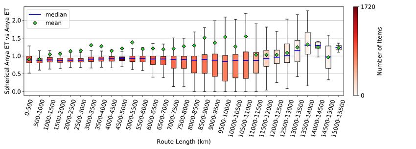
Rospotniuk and Small

algorithms take various novel approaches to partitioning the search space or post-processing
A* routes by removing nodes satisfying certain line-of-sight or collision avoidance criteria
in order to selectively reduce the total route distance compared with A*. In so doing the
resulting paths are shorter than the paths produced by graph-constrained approaches such
as A* and so return routes which are closer to optimal. Still further modifications involve
machine learning, for example whereby the measured and heuristic cost functions of A* are
learned using a Recurrent Neural Network (RNN) (Wang, Wu, Zhao, Peng, & Lin, 2019) and
myriad others which build not on A* but instead apply agent-based models with gradient
descent optimising a loss function, such as Deep Q-learning (Panov, Yakovlev, & Suvorov,
2018) or those utilising LSTMs on a training set (for instance one generated using A*)
such as (Sartoretti, Kerr, Shi, Wagner, Kumar, Koenig, & Choset, 2019)(Bency, Qureshi, &
Yip, 2019) or GAN-based approaches such as (Soboleva & Yakovlev, 2019). These Machine
Learning approaches forfeit accuracy for speed and do not guarantee optimality.

    Existing any-angle pathfinding algorithms for Euclidean space which guarantee opti-
mality include Visibility Graphs (Lozano-Pérez & Wesley, 1979), Tangent Graphs (Liu &
Arimoto, 1992), Continuous Dijkstra based approaches (Mitchell, Mount, & Papadimitriou,
1987)(Hershberger & Suri, 1999) and of course Anya (Harabor & Grastien, 2013). Anya
capitalises on the fact that all turning points on an optimal route in Euclidean space will
coincide with the corner points of obstacles, enabling the optimal path to be obtained via
online calculation of root point–interval pairs. These are projected to form visibility cones,
permitting Anya to search wide intervals of space in aggregate, rather than evaluating
visibility between neighbouring point-pairs at each grid point of the world map. This mech-
anism of projecting into space using line-of-sight intervals is what makes Anya superior in
speed to all known path-finding algorithms with an optimality guarantee and indeed, for
some maps, faster than many without this guarantee (Uras & Koenig, 2015).

    For real-world applications demanding high accuracy over long-distance voyages it be-
comes imperative to extend the approach of Anya to spherical coordinates. This opens up
an abundance of applications such as space, flight and sea voyage planning, all unsuited to
being treated as an approximation of a route in Euclidean space. Transforming the world
map representation with a Gnomonic projection whence all straight lines are great circle
lines and vice versa, at first glance permits Anya to be implemented without modification;
great-circle lines being straight lines in the Gnomonic representation of a world map. The
reason this approach falls short of achieving optimality is discussed in Appendix A. In-
stead, using Anya as a foundation it is shown that a new algorithm, Spherical Anya, can
be defined which inherits the beneficial properties of its progenitor and generalises the al-
gorithm to routes in spherical geometry. To the extent possible, the fundamental concepts
and definitions of Anya are preserved. The definition of a Grid in Spherical Anya remains
almost the same, as do the definitions of intervals, intermediate points and intersections.
Flat projections also remain virtually identical to flat projections in Anya, whereas search
nodes, cone projections, successors and observability in Spherical Anya must be defined
differently due to the great-circle geodesic of Spherical geometry. Most significantly, the
foundational theorem on which Anya depends – that of all turning points on an optimal
any-angle path being corner points – no longer holds in Spherical geometry. A new type
of non-observable cone projection must be introduced as a result, without which not all

                                              2
Optimal Any-Angle Pathfinding on a Sphere

intervals in the Spherical world map would be explored. This ensures that the optimality,
completeness and termination guarantees established for Anya extend to Spherical Anya.

2. Spherical Anya Components and Definitions
Anya pathfinding on a flat Euclidean grid takes a distinctly different approach to A-star
varieties of pathfinding which restrict travel to discrete pairwise-visible points. Instead, the
approach taken by Anya capitalises on the fact that all turning points in optimal Euclidean
paths are corner points (Mitchell et al., 1987) making the fundamental unit of abstraction
an interval of points [a, b], being either traversable or non-traversable, as opposed to a
sequence of discrete nodes. It is in this way, by defining the world map width W height H,
in terms of traversable and non-traversable intervals and subsequently generating cone– and
flat– projections along these, that Anya will select the optimal traversable path through
world map intervals without manually inspecting all rational points contained in the Farey
Sequence of order n = min(W, H). The result is an optimal pathfinding algorithm in
Euclidean space with superior speed.
    To exhibit the algorithm defining Spherical Anya it is useful to revisit and transport
the fundamental terminologies and components of Anya, these being used either directly or
adapted for Spherical Anya, where the geodesic is a great-circle line. Wherever possible the
foundational definitions of (Harabor & Grastien, 2013)(Harabor, Grastien, Öz, & Aksakalli,
2016) are maintained and adaptations and extensions are introduced only as necessitated
by the novel properties of Spherical geometry versus Euclidean geometry.
    For Spherical Anya the grid remains a planar subdivision of W × H cells. Rows are lines
of constant longitude and vertical edges are lines of constant latitude, as shown in Figure
1. This means each cell in Spherical Anya is neither square in the Euclidean sense nor the
Spherical sense; the vertical edges of the cell are not great-circle lines, albeit the horizontal
edges of the cell are, and therefore constitute the shortest path between points on the same
horizontal line, or row. Rows thus defined, obstacle edges – facing either the north or south
poles of the sphere – are not great-circle lines with the exception of edges on the equator.
Hence a great-circle line passing through the vertically aligned corner points of an obstacle
defined on the grid will in general either pass exclusively within the non-traversable bulk of
the obstacle or exclusively external to it, with the exception of the corner points themselves,
as illustrated in Figure 2.
    Of particular note is that the existence of a line of constant latitude between two points,
in addition passing adjacent only to traversable cells, does not guarantee that these two
points are visible, as illustrated for example in Figure 2(a). Instead the great-circle line,
rather than a straight line in Euclidean space, underlies the definition of visibility in Spher-
ical geometry.

Definition 1. Two points are said to be visible if they can be connected by a great-circle
line which does not pass through an obstacle or the intersection formed by two diagonally-
adjacent obstacles.

By fixing rows as lines of constant longitude, the definition of a grid interval in Spherical
Anya can remain virtually identical as for Anya.

                                               3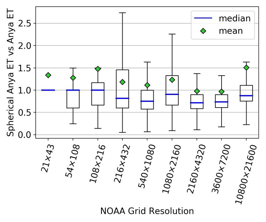
Rospotniuk and Small

                         y-axis (longitude)

                                                  x-axis (latitude)

Figure 1: An Equirectangular projection map with x-axis defining lines of constant lati-
tude and grid rows of the y-axis giving great-circle lines of constant longitude. Defining a
constant y-value as lines of longitude ensures flat projections remain virtually identical in
Spherical Anya as in Anya. Longitudinal values define rows and pairs of latitudinal values,
in combination with a row, define intervals.

Definition 2. A grid interval I is a set of contiguous and pairwise visible points drawn
from any discrete row of constant longitude on the grid. Each interval is defined in terms
of its endpoints a and b. With the possible exception of a and b, each interval contains only
intermediate non-corner points.

The grid, intervals and visibility thus defined, the next building block of Anya is the search
node. For Spherical Anya it becomes necessary to define not one but two categories of
search node, standard and adjoint, the curvature of Spherical geometry making the second
category necessary to guarantee completeness of the search space and thereby optimality of
the resulting path.

                                                        4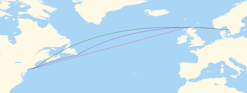
Optimal Any-Angle Pathfinding on a Sphere

     3      Obstacle in                                   3      Obstacle in
            Southern                                             Northern
            Hemisphere                                           Hemisphere
                              b                                                    b
     2                                                    2

                              a                                                    a
     1                                                    1

     0                                                    0
      0       1           2        3         4             0       1           2        3         4
   Southwards                          Northwards       Southwards                          Northwards
  (a) A great circle line between two points            (b) A great circle line between two points a
  a and b of equal latitude in the southern             and b of equal latitude in the northern hemi-
  hemisphere will always curve southwards, in-          sphere will always curve northwards, avoid-
  tersecting an obstacle with north-most edge           ing an obstacle with north-most edge upon
  upon this line. The symmetric claim holds             this line. The symmetric claim holds likewise
  likewise for a south-facing edge in the north-        for a south-facing edge in the southern hemi-
  ern hemisphere.                                       sphere.

Figure 2: Great-circle lines passing through two vertical corners of an obstacle will either
intersect only with points internal to the bulk of the obstacle or only with points external
to it, with the exception of the corner points a and b themselves.

Definition 3. A standard search node (I, r) is a tuple where r ∈ / I is a point called the root
and I is an interval such that each point p ∈ I is visible from r.

A standard node here is much the same as a node in Anya albeit with the altered definition
of visibility, being defined by the existence of a traversable great-circle path between the
root r and all points in the interval I as illustrated in Figure 3, with I := [a, b]. The interval
may be closed, as in this example, or alternatively open, or half-open. The kind of interval
used will depend on later considerations (see Definitions 5 and 6). The second category of
search node, which exists only in Spherical Anya, arises by virtue of the vertical line of an
obstacle edge generally not being the shortest path between the two corner points on the
vertical edge, as illustrated in Figure 4.

Definition 4. An adjoint search node (I, r) is a tuple where r ∈      / I is a point called the
root, which is located on the vertical edge of an obstacle, and I is a traversable interval such
that each point p ∈ I is invisible from r and furthermore the great-circle line from r to p
intersects the vertical edge twice, and only the vertical edge, including once at r.

This second kind of search node, illustrated in Figure 4, is unique to Spherical Anya and
is not required in Euclidean space where vertical edges describe straight lines and the
turning points of an optimal route will always be corner points. Neither is true in Spherical
geometry (see Section 3), where by convention the rows of the world map grid have been
fixed as great-circle lines of constant longitude and the vertical edges of obstacles are lines
of constant latitude.

                                                    5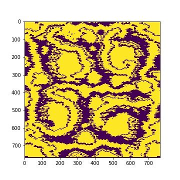
Rospotniuk and Small

                                         a                               b
                                     4

                                     3

                                     2

                                     1
                                                     r
                                     0
                                         0       1       2       3       4

Figure 3: The standard node in Spherical Anya [a, b], r is an interval I := [a, b] and a root
point r with r ∈
               / [a, b], where a traversible great-circle path exists between all points p ∈ I.
Standard nodes form the first primary abstraction of the search space, all successors along
a path from source to target destination consisting of a sequence of root points which are
either root points of a standard node (definition 3) or an adjoint node (definition 4).

                                                         a                   b
                             3

                             2

                             1

                                                             r
                             0
                                 0           1           2           3       4

Figure 4: An adjoint node exists only in Spherical Anya due to the relative curvature be-
tween the vertical constant-latitude edge of obstacles and a great-circle line drawn between
the two vertically aligned corner points of such an edge. An adjoint node is a node [a, b), r
where all cells adjacent to [a, b) are traversable and furthermore all great circle lines through
the root r and any point p ∈ [a, b) intersect the vertical edge of the obstacle twice. The
opposite scenario exists in Spherical geometry too, where no great-circle line between the
vertically aligned corners of an obstacle edge intersects the edge, excepting at the corner
points.

    The existence of adjoint nodes in Spherical geometry marks the most significant de-
parture between the underlying mathematical structure of Spherical Anya compared to
Anya. Thus far the differences have been limited; the path of shortest distance merely
being substituted for the great-circle path of Spherical geometry, the orientation of the grid
fixed explicitly to ensure rows are shortest-path lines of longitude, and the definition of
visibility similarly adapted to fit the new context. However, with the addition of adjoint

                                                         6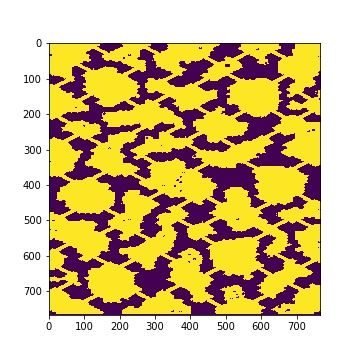
Optimal Any-Angle Pathfinding on a Sphere

nodes the divergence becomes more fundamental. This divergence is formalised in Section
3, after which it finally becomes practical to provide the concluding definitions required to
implement Spherical Anya, those of successors and projections.

3. Optimality
Lemma 1. Not all turning points on an optimal path in spherical geometry are corner
points.

Proof. By construction. It is assumed the obstacle edge is located in the northern hemi-
sphere and facing southwards as illustrated in Figure 5. All results follow identically for
the southern hemisphere and without loss of generality. For longitude, latitude (θ, φ) and
Gnomonic projection centred on the north pole (0, π2 ) we have projected coordinates

                                          cos(φ)sin(θ)
                                     x0 =
                                             sin(φ)
                                            cos(φ)cos(θ)
                                     y0 = −                                                 (1)
                                               sin(φ)

As the shortest path between any pair of points under the Gnomonic projection is a straight
line we can define the last point on the obstacle which remains visible to p as x, defined
by coordinates (θ1 , φ1 ). Target point p takes coordinates (θ2 , φ2 ). The last point on the
obstacle with direct line-of-sight to p must satisfy x · (p − x) = 0. Plugging into (1) yields
        cos(φ1 )cos(φ2 )                                   2
x · p = sin(φ              cos(θ   − θ   ) and ||x||2 = cos (φ1 ) . Solving for θ gives
              1 )sin(φ 2 )       2     1                sin 2 (φ )
                                                                1
                                                                                 1

                                                               tan(φ2 )
                                           θ1 = θ2 − cos−1                                 (2)
                                                               tan(φ1 )
This defines the point of departure from the obstacle edge. Now we show that the result
which follows from applying string-pulling holds, namely that the shortest path from the
root point r to p consists of the line segment L(r, x) defining the boundary of the obstacle
between r and x, plus the great circle line C(x, p) between x and p. The central angle
between p and any point x0 on the line θ = θ1 is given by

                 ∆σ = cos−1 sin(φ0 )sin(φ2 ) + cos(φ0 )cos(φ2 )cos(θ2 − θ1 )

                                                                                            (3)
                                −1
From identity ∂x∂
                  cos−1 (x) = √1−x  2
                                      we have that as φ0 decreases away from φ1 (recall the
equator is at φ = 0) the central angle ∆σ and therefore the great-circle distance changes by
   ∂
− ∂φ                                    0                  0
     0 which has the sign of sgn [cos(φ )sin(φ2 ) − sin(φ )cos(φ2 )cos(θ2 − θ1 )] . Substituting

in θ1 from (2) gives sgn [tan(φ1 ) − tan(φ0 )] and since φ0 < φ1 this is always positive

                               ∂
                       sgn − 0 ∆σ = sgn tan(φ1 ) − tan(φ0 ) = 1.

                                                                                             (4)
                              ∂φ
It follows that the length of this segment always increases with decreasing φ0 and we can
conclude that not only is C(x, p) the shortest traversable path between x and p but it is
also the shortest traversable path between p and any point x0 on θ = θ1 conditioned on

                                               7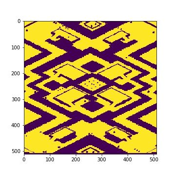
Rospotniuk and Small

φ0 < φ1 . Finally, since R · cosφ1 is the lower bound on the radius for all paths between
longitudes θ0 and θ1 in the northern hemisphere it follows that the shortest distance from
r to the line defined by θ = θ1 is R · cosφ1 (θ1 − θ0 ), which is the path defining the obstacle
boundary between those points. Hence the turning point for the optimal path between p
and r is x, as would have been concluded by string-pulling in the plane under a Gnomonic
projection.

For completeness, the practical consequence of Lemma 1 within the grid as defined for
Spherical Anya is also provided explicitly as an additional Lemma.
Lemma 2. All turning points on an optimal path in Spherical geometry are corner points
or lie within the interval defined by two vertically aligned corner points of an obstacle.
Proof. The statement is equivalent to the claim that no turning point lies within the hori-
zontal interval of a barrier. True by construction; horizontal lines are great-circle lines.

                                                                                                           θ2
                           a        p          b                                      φ2           b
θ2                                                                               φ1
                                                                                           p
                                                                                       a

                                                                                                                θ1
θ1                     x                                                                       x

                               r                                                                       r
θ0                                                                                                               θ0
                        φ1         φ2                      (0, π/2)                   decreasing φ
(a) Adjoint node [a, b), r is constructed such             (b) Gnomonic projection of the obstacle of
that [a, b) is traversable and for any p ∈ [a, b)          Figure 5(a). Great-circles are straight lines
the optimal route between r and p will consist             and without loss of generality the centre is
of a constant-latitude segment L(r, x) and a               taken as the north pole (0, π/2). Circles cen-
great-circle segment C(x, p). Hence x is the               tred on the origin are lines of constant lati-
turning point of the optimal path between the              tude, with φ decreasing to zero at the equator
root r and p, which is the basis of Lemma’s                as the radius increases.
1 and 2.

                                                    Figure 5

Lemma’s 1 and 2 provide the foundation on which to present the final components required
to implement the Spherical Anya algorithm, that of a successor, which is again adapted as
minimally as possible from that of a successor in Anya, and three categories of projection;
flat projections, standard cone projections and, uniquely to Spherical Anya, adjoint cone
projections.
    Whereas the optimal path from source to target in Anya is a sequence of pairwise visible
root points, in Spherical Anya the optimal path is a sequence of turning points which, with

                                                       8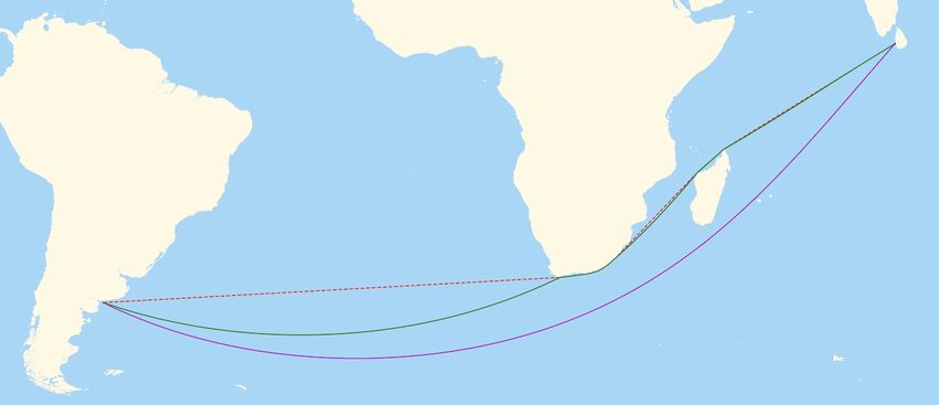
Optimal Any-Angle Pathfinding on a Sphere

the exception of turning points lying on the vertical edge of an obstacle, are also pairwise-
visible root points, by Lemma’s 1 and 2. In spite of this and the significant adaptations
made, the algorithm for calculating this sequence of optimal turning points is analogous
to Anya, where successors are constructed at each node, the mechanism by which this
occurs underlying the guarantee of completeness, optimality and termination identically in
Spherical Anya as in Anya.

4. Successors and Projections
Successors in Spherical Anya are separated into two categories, each according to the kind
of Anya node associated with it; standard or adjoint.

Definition 5. A standard successor of a search node (I, r) is a search node (I 0 , r0 ) such
that

  1. (I 0 , r0 ) is a standard node.

  2. For all points p0 ∈ I 0 there exists a point p ∈ I such that the great-circle segments
     C(r, p, p0 ) form a locally optimal route from r to p0 .

  3. r0 is the unique point closest to p0 shared by all great-circle segments C(r, p, p0 ).

  4. I 0 is maximal given the points above and the definition of a standard node.

This is the analog of a successor as defined in Anya. Due to the existence of adjoint nodes
in Spherical geometry, it is also necessary to define an adjoint successor. For all intents
and purposes these are to be treated as a standard successor in the implementation of the
Spherical Anya algorithm; the fact that no point in the node interval is visible from the
root point is relevant only insofar as local optimality of the path from adjoint node root r
through x to any point in I is in those cases accorded via Lemma 1, as is the corresponding
addition to the route g−value. Hence

                       f −value = g−value + Anya heuristic
                                  = |C(s, r1 , ..., rcurrent )| + |C(rcurrent , t)|           (5)

is throughout given by the sum of the shortest-path line segments formed by the sequence
of root points r1 , ..., rcurrent within each node from the source s, plus the Anya heuristic,
being the great-circle distance between the current root and the target t. The shortest-path
line segments C are great-circles in all cases except for adjoint nodes, where the path and
therefore the corresponding addition to the g−value is described by Lemma 1.

Definition 6. An adjoint successor of a search node (I, r) = ((a, b), r) is a search node
(I 0 , r0 ) = ((a0 , b0 ), r0 ) such that

  1. (I 0 , r0 ) is an adjoint node.

  2. I 0 is maximal given the definition of an adjoint node.

                                                    9
Rospotniuk and Small
3. Either r0 = a or r0 = b.
The mechanism by which successors are generated is via projections, analogously to
Anya, these being (i) observable (visible) cone projections, (ii) non-observable (invisible)
standard cone projections, (iii) non-observable adjoint cone projections or (iv) flat projec-
tions. Some of these projections may themselves be broken into subcategories dependent on
context. It is useful to give an overview of these in Anya, as the terminology and concepts
are foundational to both algorithms.
4.1 Projections in Anya
An observable cone projection is illustrated in Figure 6(a). This is the line-of-sight straight
line projection in Euclidean space which extends the visibility cone described by the search
node [a, b], r from an initial row to the row above, resulting in successor node [e, f ], r. Figure
6(b) provides an example of a non-observable cone projection which results in successor
(f, g], b. Here the Euclidean straight line segment L(b, f ) defines an extremal line of the
visibility cone for the successor of Figure 6(a) and the interval endpoint g is defined such
that the length of the interval (f, g] is maximal, as per the definition of a successor node.
The final manifestations of cone projections are those as illustrated in Figures 6 (c) and
(d), the former being an intermediate non-observable cone projection and the latter a (non-
intermediate) non-observable cone projection.
Flat projections, those extended from flat nodes whereby the root point lies on the
same row as the interval, are typically sub-divided into two types, being intermediate flat
projections and non-intermediate flat projections, these being referred to simply as flat
projections; see Figures 6 (e) and (f) for illustrations. An intermediate flat projection gives
rise to the successor search node (b, c], a as in Figure 6(c). Due to this interval being adjacent
to a non-traversable obstacle, it is known in advance that this search node will either be
completely traversed or ignored, as any turning point along an optimal route cannot lie
within the interval (b, c). Hence one arrives at Figure 6(d), illustrating the converse which
is a non-intermediate flat projection. Here, the successor node (c, d], a may not merely
be traversed but instead may be the site of a turning point, leading to successive cone
projections. Note that an interval may be a member of multiple successor nodes, as is the
case for intervals (b, c] and (c, d].
4.2 Projections in Spherical Anya
Projections in Spherical Anya are analogous to those in Anya but for the fact that line-of-
sight checking considers the great-circle line passing through point pairs. This differentiation
is further exposed by the appearance of adjoint successors in Spherical Anya.
Flat projections remain the same, visually, due to the convention taking rows as lines of
longitude. Where the extremal great-circle line segments C(r, a) and C(r, b) of a node [a, b], r
do not intersect an obstacle, a great-circle observable cone projection yields the standard
successor [e, f ], r much as per Anya, save for the visibility cone defining the maximal interval
I = [e, f ] now being calculated as the intercept of a great circle line through r and a with
the corresponding row of the grid, as illustrated in Figure 7(a). Similarly for the (great-
circle) non-observable cone projection (f, g], b of 7(b), defining a standard successor node
10Optimal Any-Angle Pathfinding on a Sphere
6 6
5 5
e f f g
4 4
a b a b
3 3
2 2
1 1
0 r 0 r
0 1 2 3 4 5 6 7 8 9 10 11 0 1 2 3 4 5 6 7 8 9 10 11
(a) An observable cone projection. In this instance (b) A non-observable cone projection. In this case,
the visibility cone is projected up one line to yield b being a successor root node, the cone projection
successor node [e, f ], r. of [a, b], r is found to be (f, g], b. No point within
(f, g] is visible from r.
6 6
5 5
4 4
a b c a b c d
3 3
2 2
1 1
0 r 0 r
0 1 2 3 4 5 6 7 8 9 10 11 0 1 2 3 4 5 6 7 8 9 10 11
(c) An intermediate non-observable cone projec- (d) A non-observable cone projection. In this il-
tion. The successor node (b, c], b to [a, b], r is said lustration the non-observable successor (c, d], b is
to be intermediate because it itself has only one non-intermediate because it may have multiple
successor, namely (c, d], c in Figure 6(d). successors, including successors generated via cone
projections.
6 6
5 5
4 4
a b c a b c d
3 3
2 2
1 1
0 0
0 1 2 3 4 5 6 7 8 9 10 11 0 1 2 3 4 5 6 7 8 9 10 11
(e) An intermediate flat projection. Here the (f) A non-intermediate flat projection. Here the
search node (a, b], a has been projected horizon- search node (a, b], a has been projected horizon-
tally along the same row, generating successor tally along the same row, generating successor
(b, c], a, an intermediate successor as per Figure (c, d], a. This is a non-intermediate successor as
6(c). per Figure 6(d).
Figure 6: Anya projections on a Euclidean world map
11Rospotniuk and Small
6 6
5 5
e f f g
4 4
a b a b
3 3
2 2
1 1
0 r 0 r
0 1 2 3 4 5 6 7 8 9 10 11 0 1 2 3 4 5 6 7 8 9 10 11
(a) An observable cone projection (b) A non-observable cone projection
6 6
5 5
4 4
a b c a b c d
3 3
2 2
1 1
0 r 0 r
0 1 2 3 4 5 6 7 8 9 10 11 0 1 2 3 4 5 6 7 8 9 10 11
(c) An intermediate non-observable cone projec- (d) A non-intermediate non-observable cone pro-
tion jection
c d
3
a b
2
1
r
0
0 1 2 3 4 5
(e) A non-observable adjoint cone projection.
Here the adjoint successor of the search node
[a, b], r is the adjoint node [c, d), a, whereby all
points in [c, d) are invisible from a and the inter-
val endpoint d is determined such that d is visible
from a.
Figure 7: Spherical Anya projections on a world map in Spherical geometry.
12Optimal Any-Angle Pathfinding on a Sphere
whereby f is the last point in the cone projection [e, f ], r visible to r and the interval (f, g]
is calculated to be maximal as per the definition of a successor node. Figures 7(c) and (d)
illustrate non-observable cone projections, these being visually identical to Anya. Only the
underlying metric for the geodesic between points on the same row has changed. Finally
adjoint cone projections, which are non-observable cone projections unique to Spherical
Anya, arise when a successor is an adjoint successor, as illustrated in Figure 7(e).
5. Spherical Anya Algorithm
The recipe for Spherical Anya can now be presented using the foundational components and
principles above. Globally, Spherical Anya is defined as per Anya, the difference being in
the successors generated and the underlying geodesic and line-of-sight considerations. For
easy reference, the Anya algorithm as per (Harabor et al., 2016) is reproduced below.
Algorithm 1: Anya and Spherical Anya
Require: Grid, source location s, target location t, initial root point r0 .
1: open ← {(I = [s], r0 )} . root point r0 located off the grid
2: while open is not empty do
3: (I, r) ← pop(open)
4: if t ∈ I then
5: return path to(I)
6: end if
7: for all (I 0 , r0 ) ∈ successors (I, r) do
8: if ¬should prune(I 0 , r0 ) then
9: open ← open ∪ {(I 0 , r0 )} . Successor pruning
10: end if
11: end for
12: end while
13: return null
The algorithm for calculating successors in Spherical Anya differs in form from that of
Anya due to the existence of adjoint nodes in Spherical geometry (see Algorithms 2 and 3).
In addition, the operations generate-cone-successors and generate-flat-successors
from (Harabor et al., 2016) must be replaced by their great-circle analogs from Spherical
Anya utilising great-circle geodesic and line-of-sight considerations. Furthermore, while the
pruning strategies for Anya as described in (Harabor et al., 2016) carry across to Spherical
Anya, additional pruning strategies may be applied to adjoint successors (see Algorithm 4).
Algorithm 2: Successors in Spherical Anya
1: function SUCCESSORS(n = (I, r)) . Input is current node
2: if n is the start node s then
13Rospotniuk and Small
3: return generate-start-successors(I =[s])
4: end if
5: successors ← ∅
6: if n is a flat node then
7: p ← endpoint of I farthest from r . Successor interval starts from p
8: successors ← generate-flat-successors(p, r) . Observable successors
9: if p is a corner turning point on a locally optimal path beginning at r then
10: successors ← successors ∪ generate-cone-successors(p, p, r) .
Non-observable successors
11: end if
12: if p is an adjoint turning point on a locally optimal path beginning at r then
13: successors ← successors ∪ generate-adjoint-successors(p, r) .
Non-observable successors
14: end if
15: else if n it is a cone then
16: a ← left endpoint of I
17: b ← right endpoint of I
18: successors ← generate-cone-successors(a, b, r) . Observable successors
19: if a is a corner turning point on a locally optimal path beginning at r then
20: successors ← successors ∪ generate-flat-successors(a, r) .
Non-observable successors
21: successors ← successors ∪ generate-cone-successors(a, a, r) .
Non-observable successors
22: end if
23: if a is an adjoint turning point on a locally optimal path beginning at r then
24: successors ← successors ∪ generate-adjoint-successors(a, r) .
Non-observable successors
25: end if
26: if b is a corner turning point on a locally optimal path beginning at r then
27: successors ← successors ∪ generate-flat-successors(b, r) .
Non-observable successors
28: successors ← successors ∪ generate-cone-successors(b, b, r) .
Non-observable successors
29: end if
30: if b is an adjoint turning point on a locally optimal path beginning at r then
31: successors ← successors ∪ generate-adjoint-successors(b, r) .
Non-observable successors
32: end if
33: else . If node is neither flat or cone, it is an adjoint
34: p ← endpoint of I closest to r
35: successors ← successors ∪ generate-adjoint-successors(p, r) .
Non-observable successors
36: successors ← generate-cone-successors(p, p, r) . Non-observable successors
37: end if
38: end function
14Optimal Any-Angle Pathfinding on a Sphere
5.1 Adjoint Successors
Adjoint successors occur only adjacent to the vertical edge of an obstacle, this by conven-
tion being defined as a line of constant latitude. Adjoint nodes in the northern hemisphere
exist adjacent to the south-facing edge of an obstacle and symmetrically in the southern
hemisphere exist adjacent to the north-facing edge of an obstacle (recall Figure 2). Note
also that an adjoint node for the same obstacle edge can share a root point with an adjoint
node adjacent to the same edge, the difference being only the row on which each of the
respective intervals associated with the adjoint nodes lie. The following algorithm provides
the recipe with which to calculate adjoint successors.
Figure 8 provides an illustration of the procedure, whereby all adjoint successors of the
search node [a, b], r are calculated. The first adjoint successor of this search node is [c, d), a,
the interval [c, d) calculated as per the definition of an adjoint node, such that the width
of the interval is maximal and hence such that d is visible from the new root point a but
all points p ∈ [c, d) are invisible to it. This adjoint node, having only a single possible
successor, namely [e, f ), a, is an intermediate adjoint node, as is [e, f ), a itself. Here, the
extremal point f is simply the intersection of the great circle line through a and d with the
subsequent row of the grid. Finally, projecting the great-circle lines to the next row yields
the last adjoint successor [g, h), a associated with this obstacle edge. Search node [g, h), a
is not intermediate, having more than one successor and also does not yield further adjoint
node successors.
Algorithm 3: Computing a set of adjoint successors
1: function Generate-Adjoint-Successors(an interval endpoint p, a root point r)
2: successors ← ∅
3: if p is a corner point then
4: r0 ← p
5: else
6: r0 ← r
7: end if
8: p0 ← a point from adjacent row, farthest and non-observable one from r0
9: Imax ← maximum closed interval beginning at p0 and non-observable from r0
10: for all I ∈ {split Imax at each corner point} do
11: n0 ← a new search node with interval I and root point r0
12: successors ← successors ∪ I
13: end for
14: return successors
15: end function
15Rospotniuk and Small
6
g h
5
e f
4
c d
3
a b
2
1
0 r
0 1 2 3 4 5
Figure 8: A series of intermediate adjoint nodes which are calculated in the process of
generating the final non-intermediate adjoint node [g, h), a.
Algorithm 4: Intermediate node pruning
1: function Is-Intermediate(n = (I, r))
2: if n is a flat node then
3: p ← endpoint of I furthest from r
4: if p is a corner turning point for a locally optimal path with prefix hr, pi then
5: return false . n has at least one non-observable successor; it cannot be
intermediate
6: end if
7: else if n is an adjoint node then
8: p0 ← endpoint of I closest to r
9: if p0 is a corner point then
10: return false . n has at least one non-observable successor; it cannot be
intermediate
11: end if
12: else
13: if I has a closed endpoint that is also a corner point then
14: return false . n has at least one non-observable successor; it cannot be
intermediate
16Optimal Any-Angle Pathfinding on a Sphere
15: end if
16: I 0 ← interval after projecting r through I
17: if I 0 contains any corner points then
18: return false . n has at least one non-observable successor; it cannot be
intermediate
19: end if
20: end if
21: return true
22: end function
5.2 Spherical Anya Algorithm: Examples
We provide examples which illustrate how Spherical Anya works in practice by illustrating
all successors for a given root node as would be necessary in an implementation of the
Spherical Anya algorithm, search nodes and their corresponding successors comprising the
fundamental units of the search algorithm.
5.2.1 Successors of a flat search node
In the following scenario the Spherical Anya algorithm is required to generate all successors
of the flat search node (r, a], r ≡ (0, 2], r, of Figure 9. As the root point of the node is on the
same row as the interval, the first projections are flat projections, generating flat successors
until the wall of Figure 9(d) interrupts progress. In this instance the wall is created by the
existence of two diagonally adjacent non-traversable cells centred on the point e = (7, 2) of
Figure 9(d). Not all of these successors survive however, those not containing the target
point and being intermediate by virtue of their adjacency to a non-traversable cell, as (b, c], r
is in Figure 9(b) and (d, e], r is in Figure 9(d), being discarded. These cannot precede a
turning point on any optimal route. The search node (d, e], r of Figure 9(d) is in addition
a cul-de-sac node. It has no successors, and the target does not lie in the interval (d, e].
All flat successors being thus generated, the Spherical Anya algorithm generates all flat-
to-adjoint projections and flat-to-cone projections. These occur at the farthest corner of
each non-traversable interval from the root r, along the same row and prior to the edge
defined by the wall. In this example, flat-to-adjoint and flat-to-cone projections will be
generated by Spherical Anya at each of the new root points a = (2, 2) and c = (5, 2), as
illustrated in figures 9(e)–(h).
5.2.2 Successors of a cone search node
In the next example, the search node [a, b], r is now a cone search node, as illustrated in
Figure 10, as the root point r no longer lies on the same row as the interval [a, b]. The
first successor of this is calculated as the great-circle cone projection to the next row of
the map, yielding successor [c, d], r of Figure 10(a) with the same root point as its parent.
Subsequent to the (non-adjoint) cone projection yielding search node [c, d], r all invisible
cone projections must be generated, these being invisible from root point r. This is achieved
17Rospotniuk and Small
3 3
r a b r a b c
2 2
1 1
0 0
0 1 2 3 4 5 6 7 8 0 1 2 3 4 5 6 7 8
(a) An observable flat projection. Not being ad- (b) An intermediate flat projection. Being adja-
jacent to a non-traversable cell, this successor cent to a non-traversable cell this successor node
[2, 4], r is added to the list of successors of [0, 2], r. is discarded.
3 3
r a c d r a d e
2 2
1 1
0 0
0 1 2 3 4 5 6 7 8 0 1 2 3 4 5 6 7 8
(c) An observable flat projection yielding successor (d) An intermediate flat projection. This interval
[5, 6], r. is adjacent to a cul-de-sac wall formed by two diag-
onally adjacent obstacles, and hence is discarded.
3 3
r a r a
2 2
1 f g 1 g h
0 0
0 1 2 3 4 5 6 7 8 0 1 2 3 4 5 6 7 8
(e) An adjacent flat-to-cone projection. The root (f) A non-adjoint standard cone projection pro-
point is r0 , invisible to all points in the node in- vides the final successor with root point r0 and
terval I, because a great-circle line intersects the interval J. All points in J are visible with respect
neighbouring obstacle twice. to r0 .
3 3
r a c r a c
2 2
1 i j 1
j k
0 0
0 1 2 3 4 5 6 7 8 0 1 2 3 4 5 6 7 8
(g) An adjacent flat-to-cone projection. The root (h) A non-adjoint standard cone projection pro-
point is r0 , invisible to all points in the node in- vides the final successor with root point r0 and
terval I, because a great-circle line intersects the interval J. All points in J are visible with respect
neighbouring obstacle twice. to r0 .
Figure 9: All successors of search node (r, a], r are illustrated to provide an example of
successor generation in Spherical Anya.
18Optimal Any-Angle Pathfinding on a Sphere
by forming the search node (d, e], b of Figure 10(b) by searching right from d, the last point
on row 3 visible to r.
Once there are no further options for expanding a great-circle visibility cone to the
third row of the map the search continues horizontally, generating flat, intermediate, flat-
to-adjoint and flat-to-cone projections. This process continues along row 2 until a wall is
reached, or as is the case in this scenario, the edge of the map. The first flat projection
is (b, f ], b, this being the case because the new root point b is selected due to being the
extremal edge of the parent interval. Node (b, f ], b however, being adjacent to an obstacle,
is intermediate and not added to the list of successors. The subsequent successor (f, g], b,
while not being adjacent to a non-traversable cell in this instance, is also not added to the
list of successors for the parent node [a, b], r because (f, g], b is adjacent to the edge of the
map and therefore is a successor without successors. Given the target doesn’t lie in the
interval (f, g] it is a cul-de-sac, and hence dropped as well. The only remaining successors
in this scenario are therefore the flat-to-adjoint and flat-to-cone successors of Figures 10(e)
and (f).
6. Results
Results are reported on execution time (ET) and number of tiles crossed (CT), a tile be-
ing a single unit of the world map grid. Statistics are calculated for 4 game maps plus
city/street maps and four random maps, in addition to the Earth maps determined by the
NOAA bathymetric dataset at several resolutions. Comparisons and benchmarks to exist-
ing Euclidean approaches being already reported in (Harabor et al., 2016), the following
results compare exclusively the difference between Anya and Spherical Anya. Both algo-
rithms are implemented in Python and executed on an AWS EC2 Dual Core Intel Xeon
Platinum 8000 “R5.Large” Instance with 16GB of RAM. The definition of the benchmark
is designed to measure the relative expense in time and route length of achieving optimality
in Spherical geometry with the application of Spherical Anya, compared to applying Anya
with the assumption that the underlying geometry is Euclidean. We highlight that such a
comparison is dependent on programming language and employed data structures, making
all benchmark statistics herein indicative in Python only. We do not provide a comparison
across programming languages, for which these figures would likely be different. For any
world map defined as a list of coordinate pairs [(x1 , y1 ), ...., (xm , yn )] for an n × m world,
each item is assigned a value of zero for a non-traversable cell and one for a traversable cell.
For the application of Anya, source and target points are selected uniformly from the set
of traversable cells, and Anya is applied on the world map directly, considering each cell to
be a uniform square of unit length. The resulting route is mapped to Spherical coordinates
with the linear mapping, in degrees, being
2xi
xlat
i = 90 −1
m
2yj
yjlon = 180 −1 . (6)
n
19Rospotniuk and Small
c d d e
3 3
a b a b
2 2
1 1
r r
0 0
0 1 2 3 4 5 0 1 2 3 4 5
(a) An observable cone projection. (b) Non-observable cone projection.
3 3
a b f a b f g
2 2
1 1
r r
0 0
0 1 2 3 4 5 0 1 2 3 4 5
(c) Non-observable intermediate flat projection. (d) Non-observable flat projection.
3 3
a b f a b f
2 2
1 h i 1 j
i
r r
0 0
0 1 2 3 4 5 0 1 2 3 4 5
(e) Non-observable adjoint flat-to-cone projection. (f) Non-observable standard (non-adjoint) flat-to-
cone projection.
Figure 10: A series of flat, flat-to-adjoint and flat-to-cone projections define the successors
to the illustrated search node [a, b], r.
Results are shown for two distinct recipes for connecting the root points returned from Anya
to form a route in Spherical geometry. Recipe 1 connects root points directly with great-
circle lines. A consequence of this is that Recipe 1 achieves routes whose total length is closer
to that of the optimal route returned by Spherical Anya, but with a relatively high number
of routes intersecting non-traversable cells. We refer to routes as legal whereupon this does
not occur. All routes generated by Spherical Anya in Spherical geometry are both legal and
optimal whereas this is not the case for Anya – Anya not being designed for application
in Spherical geometry and therefore guaranteeing neither legality nor optimality of routes.
Recipe 2 enriches the route segments returned by Recipe 1 which intersect non-traversable
cells with additional synthetic root points every arc-second along a straight (Euclidean) line
between the root points where this occurs. Finally a great-circle line is assumed between
20Optimal Any-Angle Pathfinding on a Sphere
Spherical Anya vs. Anya ET (All Routes)
Benchmark #Maps #Instances
% less Min Q1 Median Mean Q3 Max StDev
Starcraft 75 18,068 35.27 0.003 0.806 1.188 2.048 2.018 60.019 3.451
Dragon Age 2 67 14,369 31.58 0.006 0.857 1.000 1.368 1.525 56.366 1.359
Baldurs Gate II, scaled to 512 × 512 75 17,580 31.18 0.005 0.861 1.000 1.561 1.690 53.262 1.798
Warcraft III, scaled to 512 × 512 36 7,992 38.63 0.015 0.833 1.000 2.881 1.367 60.421 6.346
City/street Maps 90 21,515 33.53 0.014 0.804 1.261 3.424 3.103 60.442 6.160
Random 10%, 256 × 512 75 18,241 53.37 0.000 0.476 0.911 1.510 1.686 13.807 1.906
Random 20%, 256 × 512 75 18,305 46.48 0.000 0.593 1.052 1.587 1.876 13.782 1.724
Random 30%, 256 × 512 75 18,175 41.67 0.001 0.725 1.112 1.419 1.757 13.724 1.209
Random 40%, 256 × 512 75 16,091 31.73 0.000 0.944 1.100 1.207 1.359 13.582 0.694
NOAA bathymetry, 10800 × 21600 1 22,060 74.20 0.003 0.796 0.905 1.630 1.000 90.596 5.085
Table 1: Execution time (ET) on a series of standard game maps, random maps and NOAA
bathymetry is calculated from randomly sampled source and target points and alternatively
considered to be defined over Euclidean and Spherical geometry. The column “% less”
indicates the percentage of routes whereupon Spherical Anya ET is less than Anya ET.
Spherical Anya vs. Anya Route Length (Recipe 1)
Benchmark #Maps #Instances
% less Min Q1 Median Mean Q3 Max StDev
Starcraft 75 18,068 56.98 0.132 0.990 1.000 0.977 1.000 1.509 0.069
Dragon Age 2 67 14,369 36.27 0.162 1.000 1.000 0.995 1.000 2.047 0.047
Baldurs Gate II, scaled to 512 × 512 75 17,580 36.71 0.191 0.999 1.000 0.997 1.000 5.528 0.082
Warcraft III, scaled to 512 × 512 36 7,992 29.24 0.279 0.998 1.000 1.008 1.000 5.201 0.143
City/street Maps 90 21,515 60.54 0.180 0.910 0.996 0.947 1.000 5.983 0.137
Random 10%, 256 × 512 75 18,241 96.75 0.049 0.738 0.931 0.834 0.988 1.003 0.206
Random 20%, 256 × 512 75 18,305 95.96 0.046 0.748 0.932 0.836 0.988 1.002 0.205
Random 30%, 256 × 512 75 18,175 93.84 0.053 0.792 0.949 0.851 0.994 1.001 0.204
Random 40%, 256 × 512 75 16,091 84.41 0.024 0.965 0.998 0.924 1.000 1.001 0.172
NOAA bathymetry, 10800 × 21600 1 22,060 37.44 0.320 1.000 1.000 0.997 1.000 1.103 0.017
Table 2: Route Length (RL) on a series of standard game maps, random maps and NOAA
bathymetry is calculated from randomly sampled source and target points and alterna-
tively considered to be defined over Euclidean and Spherical geometry. The table includes
both illegal and legal Anya routes generated by interpolating between route points with a
great-circle (Recipe 1). The column “% less” indicates the percentage of routes whereupon
Spherical Anya RL is less than Anya RL. The ratio being greater than 1 occurs when non-
legal routes are permitted, i.e. when Anya generates a route which in Spherical geometry
intersects at least one non-traversable cell. All routes generated by Spherical Anya are legal.
root-point pairs in the enriched set. Recipe 2 produces fewer illegal routes than Recipe 1,
albeit at the expense of generating legal routes with distance greater than those produced
by Recipe 1.
For Spherical Anya the world map is first transformed into Spherical coordinates and
the shortest-distance route is subsequently calculated. Under such circumstances it is guar-
anteed that Spherical Anya will find the optimal legal route whereas Anya may not, the
relevant question here being at what cost? What is the cost in execution time (ET) and
route length (RL) of achieving optimality in Spherical geometry, compared with the sim-
plification of assuming a Euclidean geodesic on a “flat earth”.
Results are provided in Tables 1, 2, 3 and 4. The standard benchmark game maps
which have been selected are Starcraft, Dragon Age 2, Baldurs Gate II and Warcraft III,
with source and target uniformly selected with replacement an #Instances number of times
21Rospotniuk and Small
Spherical Anya vs. Anya Route Length (Recipe 2)
Benchmark #Maps #Instances
% less Min Q1 Median Mean Q3 Max StDev
Starcraft 75 18,068 91.22 0.131 0.969 0.993 0.965 0.999 1.000 0.072
Dragon Age 2 67 14,369 86.90 0.162 0.996 0.999 0.990 1.000 1.000 0.043
Baldurs Gate II, scaled to 512 × 512 75 17,580 75.04 0.191 0.989 0.999 0.984 1.000 1.000 0.045
Warcraft III, scaled to 512 × 512 36 7,992 53.32 0.279 0.938 1.000 0.954 1.000 1.000 0.079
City/street Maps 90 21,515 85.94 0.176 0.870 0.971 0.917 0.999 1.000 0.111
Random 10%, 256 × 512 75 18,241 99.27 0.049 0.737 0.930 0.833 0.988 1.000 0.206
Random 20%, 256 × 512 75 18,305 99.62 0.046 0.748 0.931 0.836 0.988 1.000 0.205
Random 30%, 256 × 512 75 18,175 99.86 0.053 0.792 0.948 0.851 0.994 1.000 0.204
Random 40%, 256 × 512 75 16,091 99.93 0.024 0.965 0.998 0.924 1.000 1.000 0.172
NOAA bathymetry, 10800 × 21600 1 22,060 49.79 0.320 0.999 1.000 0.993 1.000 1.000 0.024
Table 3: Distribution of Route Length Ratios (including illegal routes) where Anya routes
are generated by linear enrichment every 1 arc-second between root point pairs for which
a great-circle connection would yield an intersection in Spherical geometry (Recipe 2).
Compared to the mechanism of Table 2 this simultaneously reduces the number of illegal
routes generated by Anya and increases the corresponding route lengths further from those
of Recipe 1. The column “% less” indicates the percentage of routes whereupon Spherical
Anya route length is less than Anya route length. The opposite occurs for illegal Anya
routes.
Spherical Anya vs. Anya Route Length (Exclusive, Recipe 1)
Benchmark #Instances
% less Min Q1 Median Mean Q3 Max StDev
Starcraft 12,594 81.75 0.132 0.970 0.997 0.964 1.000 1.000 0.077
Dragon Age 2 9,511 54.80 0.162 0.999 1.000 0.990 1.000 1.000 0.049
Baldurs Gate II, scaled to 512 × 512 12,454 51.81 0.191 0.996 1.000 0.987 1.000 1.000 0.045
Warcraft III, scaled to 512 × 512 6,295 37.12 0.279 0.989 1.000 0.978 1.000 1.000 0.052
City/street Maps 17,094 76.20 0.180 0.875 0.974 0.922 1.000 1.000 0.107
Random 10%, 256 × 512 17,997 98.07 0.049 0.734 0.929 0.832 0.987 1.000 0.206
Random 20%, 256 × 512 17,860 98.35 0.046 0.740 0.927 0.832 0.986 1.000 0.206
Random 30%, 256 × 512 17,289 98.65 0.053 0.777 0.941 0.844 0.990 1.000 0.206
Random 40%, 256 × 512 13,716 99.02 0.024 0.945 0.995 0.911 1.000 1.000 0.183
NOAA bathymetry, 10800 × 21600 19,924 41.46 0.320 1.000 1.000 0.996 1.000 1.000 0.017
Table 4: Distribution of Route Length Ratios excluding illegal routes wherein the Anya
route is shorter than the Spherical Anya route. This occurs if and only if Anya returns a
route which intersects a non-traversable cell at least once.
22Optimal Any-Angle Pathfinding on a Sphere
over a #Maps number of maps for each game. These game maps have features which are
interesting to study in their own right and we do not dwell on them here. For example
Real Time Strategy games such as Starcraft contain large, obstacle free, traversable areas
with choke points (see Figure 11) whereas Role-playing games such as Baldurs Gate II
are maze-like. Figure 12 illustrates the ratio of Spherical Anya ET over Anya ET for
these game maps and City/street maps. Also presented are results from random maps (see
Figure 13). Note that these maps are originally 2D maps, repurposed here for illustrating
the statistical relationship between Anya and Spherical Anya given (i) different recipes for
creating routes in Spherical geometry from the root points yielded by Anya (ii) different
underlying measures for line-of-sight checking and finally, but significantly (iii) differing
world maps. Beyond this statistical comparison it is the sea-voyages based on the NOAA
bathymetric relief map of Earth (NOAA, 2009) which additionally bear practical utility in
real world applications.
These simulations show that Spherical Anya is mostly similar in execution time to Anya,
but on average it is slower (see Table 1). Moreover the median ET of Spherical Anya be-
ing faster or slower than Anya is strongly dependent on the features of each world map.
The reward is only occasionally speed but always legality and optimality, Spherical Anya
producing routes on average over 7.4% shorter than routes generated by Anya across all
maps using Recipe 1 (see Table 4). The statistics for Random maps at 10%, 20%, 30%,
40% clearly show the importance of the features of the world map as well as the number
of tiles crossed (see Figure 13), the percentage here defining the Bernoulli random variable
determining the existence of a non-traversable coordinate in the world map. Random maps
produce route length ratios smaller than those of other maps and suffer a high RL ratio
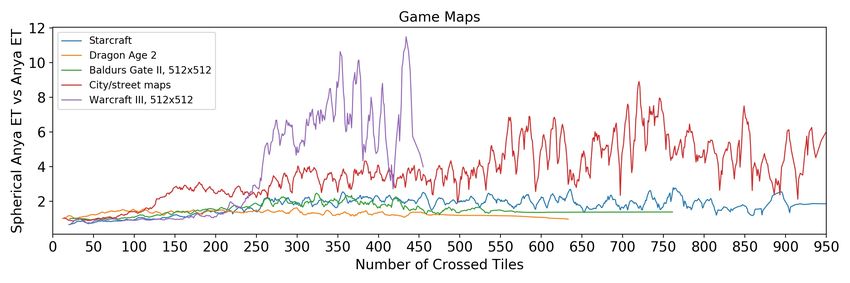
standard deviation compared to other world maps. More importantly for practical applica-
tions such as the navigation of seafaring vessels, median ET for Spherical Anya is slightly
less than Anya and average ET is higher for almost all world map resolutions and route
lengths (see Figures 14 and 15). Never generating routes which intersect land, as Anya does
in Spherical geometry, Spherical Anya always returns the optimal route. Refer to Appendix
B, Figures 18 and 19 for illustrations of instances of ocean voyages. In summary, Spherical
Anya being always optimal and producing legal routes in Spherical geometry, is faster on
most routes compared with Anya for sea-faring routes, but more often it is slower.
7. Conclusion
It has been shown that a fast, efficient and optimal pathfinding algorithm for Spherical
geometry exists in the form of Spherical Anya, a new online pathfinding algorithm which
modifies and extends the principles of the Anya algorithm in Euclidean geometry. Modifi-
cations include the obvious change from the Euclidean geodesic to the great-circle geodesic
of Spherical geometry. Further changes are a consequence of this, for instance one can
no longer rely upon all turning points on an optimal route being corner points, and the
existence of adjoint search nodes and successors which do not exist in Anya. The Spherical
Anya algorithm for optimal pathfinding in Spherical geometry is described and illustrated
with examples, and the primary mathematical consequence of the transition from Euclidean
geometry to Spherical geometry is stated and proven. All remaining terminology, proce-
23Rospotniuk and Small
(a) A Starcraft map instance, with traversable re- (b) A second example of a Starcraft map instance.
gions coloured yellow and non-traversable regions Here the ratio of non-traversable regions compared
coloured purple. This can be considered either a to traversable regions is 38.37%.
flat map, as was originally intended, or a map in
Spherical geometry via the mapping of equation
(6).
(c) A third example of a Starcraft map instance. (d) A final example of a Starcraft map instance.
The ratio of non-traversable cells compared to The ratio of non-traversable cells compared to
traversable cells is 42.11%. The average length of traversable cells is 1.38%. The average length of
a route for this map is 10,920.2 km in Euclidean a route for this map is 10,606.3 km in Euclidean
geometry and 10,829.7 km in Spherical geometry. geometry and 9,577.0 km in Spherical geometry.
To compare, the median distance over all Starcraft The median ratio over all Starcraft map instances
map instances in Euclidean and Spherical geome- is 25.77%.
try is 13,822.4 km and 13,454.9 km respectively.
Figure 11: Starcraft Real Time Strategy game map instance examples.
24You can also read